Distributed Recoverable Sketches

Abstract
Sketches are commonly used in computer systems and network monitoring tools to provide efficient query executions while maintaining a compact data representation. Switches and routers maintain sketches to track statistical characteristics of the network traffic. The availability of such data is essential for the network analysis as a whole. Consequently, being able to recover sketches is critical following a switch crash.
In this paper, we explore how nodes in a network environment can cooperate to recover sketch data whenever any of them crashes. In particular, we focus on frequency estimation linear sketches, such as the Count-Min Sketch. We consider various approaches to ensure data reliability and explore the trade-offs between space consumption, runtime overheads, and traffic during recovery, which we point out as design guidelines. Besides different aspects of efficacy, we design a modular system for ease of maintenance and further scaling.
A key aspect we examine is how nodes update each other about their sketch content as it evolves over time. In particular, we compare between periodic full updates vs. incremental updates. We also examine several data structures to economically represent and encode a batch of latest changes. Our framework is generic, and other data structures can be plugged-in via an abstract API as long as they implement the corresponding API methods.
Keywords and phrases:
Sketches, Stream Processing, Distributed Recovery, Incremental Updates, Sketch PartitioningCopyright and License:
2012 ACM Subject Classification:
Networks Network monitoring ; Computer systems organization Dependable and fault-tolerant systems and networks ; Computer systems organization ReliabilityAcknowledgements:
We would like to thank the anonymous reviewers for their insightful comments.Funding:
This work was partially funded by the Israeli Science Foundation grant #3119/21.Editors:
Silvia Bonomi, Letterio Galletta, Etienne Rivière, and Valerio SchiavoniSeries and Publisher:
1 Introduction
Network monitoring is a crucial part of network management. Effective routing, load balancing, as well as DDoS, anomaly and intrusion detection, are examples of applications that rely on monitoring network flows’ frequencies [3, 10, 13, 14]. Internet flows are often identified by the source and destination IP addresses. Yet, IPv4 5-tuple (, , , , ) can be used, uniquely identifying each connection or session [17].
Monitoring tools track a significant amount of flows, updating the frequency count of every flow upon each of its packets’ arrival [2]. Hence, maintaining exact counter-per-flow is often not feasible due to the high line rates of modern networks as well as lack of space of SRAM memory. To overcome these limitations, it is common to trade the accuracy for memory space with sketching algorithms, that utilize hashing to summarize traffic data using fewer counters and without explicitly storing flows’ identifiers, e.g., Count Sketch [4], Spectral Bloom Filter [7], and Count-Min Sketch [8]. Count-Min Sketch (CMS) is a popular sub-linear space data structure for flow size estimation. It uses pairwise-independent hash functions to map flows to frequencies, while sub-linear space is achieved at the expense of over estimating some flows’ frequencies due to hash collisions. Given a stream of items and accuracy parameters , CMS guarantees that the estimation error for any flow (distinct item) is bounded by , with probability at least .
Switches and routers constantly produce statistics of the tracked traffic. The availability of such data is essential for the network analysis as a whole, and to enable continuous as well as long term survivability of its applications. The ability to recover the statistics after a crash failure is therefore highly desirable. Obviously, ensuring such information durability requires a certain level of redundancy and replication. However, tracing and processing information at the high line rate of modern networks may consume significant networking, computation, and storage resources. On the other hand, the fact that we specifically target sketches, may offer opportunity to reduce these costs compared to direct utilization of common techniques used for general data availability. To that end, in this work we explore various approaches to ensure data survivability of fast updating sketches in terms of their computational costs, communication cost under normal operation, recovery communication cost (after a failure), and storage overhead.
Contributions.
Our goal is to design a flexible distributed fault tolerant software system consisting of fully functional switches, each maintaining its own local sketch (referred as data node), while sharing different partitions of its sketch with other switches (referred as redundant nodes) for backup. In case of switch’s crash failure, the others will contribute to the recovery process, restoring the latest backup of failed sketch. One of our goals is to provide a modular system having simple design, which is easy to maintain and further scale. Modularity is inherent in our design, which relies on swapable building blocks, providing a variety of configurations and settings, as well as extendability through API.
During the pre-processing stage, the global configuration is generated based on user-specified parameters. Further, we assume that all nodes are globally configured with the same parameters and same hash functions as well, resulting in identical sketch structure. Additionally, we assume that all the nodes comply with the protocol. Given the physic parameters associated with system topology, such as number of switches, our framework enables tuning the necessary parameters for the preferred performance goals.
To enable self-configuration we are looking for algorithms that optimize the trade-offs between space redundancy overhead, communication overhead during redundancy maintenance, and the amount of recovery traffic after a node’s failure. To this end, we distinguish between the redundant space required to store the redundant sketches, and the extra local space required to represent a batch of delayed items, used for incremental updates.
Redundant information can be constructed by summing the sketches into a sum sketch, having the same structure, but with longer counters to count up to the sum of items in data streams it covers. Inspired by RAID [5] we introduce simple yet scalable method to generate redundant sums to tolerate any number of concurrent failures, as described in 5.1.1. Our generation method has a property of optimal erasure code, and its small coefficients imply fast multiply operations. As pointed out in 2.2, since our work is sketch-aware, we are able to use less space than required with RAID, while buffering the changes into a batch.
Paper organization.
Section 2 shortly covers the related work, and the associated properties we rely on. In Section 3 we formulate the model and its key entities, while Section 4 highlights the key aspects of efficacy we focus on during the system design. Section 5 describes the two redundancy strategies and a trade-off between the redundant space and the recovery traffic. In Section 6 we introduce several data structures to economically represent a batch of latest changes. Finally, in Section 7 we conclude and discuss some future work.
2 Background and Related Work
2.1 Count-Min Sketch
Count-Min Sketch (CMS) [8], is a probabilistic data structure for summarizing data streams, which can be used to identify heavy hitters (frequent items). Using several hash functions and corresponding arrays of counters, it responds to a point query with a probably approximately correct answer by counting first and computing the minimum next. This ensures that the overestimation caused by hash collisions is minimal.
Given user-specified parameters , a CMS is represented by a matrix of initially zeroed counters, , where and . Additionally, hash functions are chosen uniformly at random from a pairwise-independent family, mapping each item to one cell, for each row of .
When an update arrives, meaning that item is updated by a quantity of , then is added to the corresponding counters, determined by for each row . Formally, set .
The answer to a point query is given by . The estimate has the following guarantees: () , where is the true frequency of within the stream, and () with probability at least , , where is the total number of items in the stream. Alternatively, the probability to exceed the additive error is bounded by , i.e., .
2.2 RAID
Chen, Lee, Gibson, Katz and Petterson described in 1994 the seven disk array architectures called Redundant Arrays of Inexpensive Disks, aka RAID levels 0-6 [5]. These schemes were developed based on the two architectural techniques used in disk arrays: striping across multiple disks to improve performance, and redundancy to improve reliability. Data striping results in uniform load balancing across all of the disks, while redundancy in the form of error-correcting codes (like parity, Hamming or Reed-Solomon codes) tolerates disk failure. Parity information can be used to recover from any single disk failure. RAID 4 concentrates the parity on dedicated redundant disk, while RAID 5 distributes the parity uniformly across the disk array. Thinking of a redundant disk as holding the sum of all the contents in data disks, when a data disk fails, all the data on non-failed disks can be subtracted from that sum, and the remaining information must be the missing one. RAID 6, also called redundancy, uses Reed-Solomon codes to tolerate up to two disk failures.
Our work is inspired by RAID, but optimized to the realm of sketches, which in networking applications, must cope with extremely fast update rates across the network. In RAID, the parity can be either reconstructed from scratch or updated incrementally by applying the differences in parity between the new and old data. This general technique can be applied to sketches that process data streams and send periodic updates in cycles. It can be further optimized with compact encoding to reduce the communication cost when only few changes occurred. Yet, two data sketches are required to compute the differences in parity: the original sketch, whose content is updated during the normal execution, and the latest backup from the prior update cycle, aka the new and old data.
As our work is sketch-aware, we use simplified design focusing on integers instead of parity bits. With linear sketches we are able to update the redundant nodes in incremental manner, producing the sums as if were calculated from scratch. To this end, next to its original sketch, each data node holds only the ongoing changes of a cycle.
2.3 Batching and Buffering
We consider the general message-passing model with and operations111Alternatively, one can think of an RDMA-like and model., and assume that messages are sent over reliable communication links, similar to TCP/IP or QUIC, that provide an end-to-end service to applications running on nodes. Data nodes could update the redundant nodes on each item arrival by simply forwarding, as they process their data streams. An IP packet is the smallest message entity exchanged via the Internet Protocol across IP network. As each message consists of a header and data (payload), it is reasonable to send updates whenever there are enough changes to fill an IP packet. This would increase network throughput by reducing the communication overhead, associated with transmitting a large number of small frames. Batching and buffering are commonly used techniques, where the events are buffered first and sent as a batch operation next. With batch publishing strategy, RabbitMQ publisher [12] batches the messages before sending them to consumers, reducing the overhead of processing each message individually.
To maintain the redundant information efficiently, we consider periodic updates of incremental changes and examine several data structures to economically represent and encode a batch. Batch may contain only a small portion of overall flows, making it feasible to maintain exact counter-per-flow (e.g., using a compact hash table [1]). We begin with traditional buffering of items as they arrive, and then switch to flows, grouping the items by their identifiers while maintaining their accumulated frequencies using key-value pairs.
2.4 Compact Hash Tables
Dictionaries are commonly used to implement sets, using an associative array of slots or buckets to store key-value pairs, with the constraint of unique keys. The most efficient dictionaries are based on hashing techniques [15], but hash collisions may occur when more than one key is mapped to the same slot of a hash table. Different implementations exist aiming to provide good performance at very high table load factors. A load factor of a hash table is defined as the ratio between the number of elements occupied in a hash table and its capacity, signifying how full a hash table is. A hash table has to rehash the values once its load factor reaches the load threshold, i.e., the maximum load factor, which is an implementation-specific parameter. To avoid collisions, some extra space is required in the hash table, by having the capacity greater than the number of elements at all times.
We consider an abstract compact hash table having load threshold. High-performance hash tables often rely on bucketized cuckoo hash table, due to featuring an excellent read performance by guaranteeing that the value associated with some key can be found in less than three memory accesses [16]. While the original Cuckoo hashing [15] requires the average load factor to be kept less than , in Blocked cuckoo hashing [9], using four keys per bucket increases the threshold to .
3 Model Description
We assume a collection of nodes, each with a unique identifier known to all others, whose goal is (possibly, among other things) to monitor streams of data items flowing through them. For example, these nodes could be routers in a network, or servers in a decentralized scalable web application. We also assume that the nodes are equipped with reliable memory and can communicate with each other by exchanging messages over reliable communication links. That is, each message sent by a non-failed node to another non-failed node is eventually delivered at its intended recipient using an end-to-end communication service. Otherwise, we detect it as failed node, and can initiate the recovery procedure to reconstruct its sketch up to the latest restoring point. We focus on erasures only, due to reliable memory and communication links, as well as error-correction and retransmissions provided by the lower layer protocols, which are out of our scope.
Every stream , for , is modeled as a sequence of items , each carrying an identifier and possibly additional data that is irrelevant to our work, and is therefore ignored from this point on. At any given point in time , part of each stream has already arrived, while the rest of the stream is still unknown. To avoid clatter, whenever is clear from the context, we omit it. Within these streams, we refer all items having the same identifier as instances of a particular flow, denoted as , or simply referred by its identifier . The goal of each node is to track the frequency of every flow within its stream , i.e., to “count” the number of items having identifier that flowed through it so far. To reduce the space overhead, nodes only maintain an estimation of each flow’s frequency through Count-Min Sketches, which are configured with the same global parameters and the same hash functions as well. Upon a point query for a given flow , whose true frequency in a stream after arrivals is , the CMS maintained by a node would return the estimate , such that with probability at least .
Our goal is to share redundant information regarding each node’s sketch elsewhere, so if that node fails, it would be possible to recover the missing data. To that end, from now on we refer to nodes holding sketches capturing stream data flowing through them as data nodes. In particular, we have data nodes. We also introduce into the model redundant nodes, whose goal is to store redundant information needed for recovery of failed sketches.
We consider two main use cases: () redundant nodes only store redundant information, in which case we refer to them as dedicated redundant nodes, and assume that they too can communicate reliably with each other as well as with all data nodes; alternatively, () each data node may serve as a redundant node too, in which case we have distributed redundancy, where a set of redundant nodes is a subset of data nodes. In case (), the roles are exclusive, i.e., a node can be either data or redundant, but not both. Hence, a pure redundant node can be realized as a centralized controller or backup server. In case (), in contrast to RAID 5, every node holds its own original sketch entirely, and may or may not provide backup services for others. With this approach, the nodes perform as a distributed backup service storing redundant sum sketches next to their original sketches. For ease of reference, Table 1 summarizes the notations presented here as well as later in this paper.
4 Design Guidelines
During the system design we explore some trade-offs, which among other savings might reduce the total environmental impact, in terms of resource consumption.
- Storage.
-
Trade the recovery traffic for redundant space, using sum sketches instead of full replicas. Following the approach from Section 1, redundant information can be constructed by summing original (data) sketches into redundant sum sketches, requiring less memory than storing full replicas.
- Communication.
-
Reduce maintenance traffic, using incremental updates organized in batches. We generally prioritize to reduce unnecessary communication traffic during runtime. Thus, we also embrace compact message encoding and early transmissions avoidance.
- Runtime.
-
Reduce the number of rehash operations and improve performance, providing a data structure with an initial capacity upon memory allocation. Don’t forget to take into account the load threshold of a data structure, 1.0 by default. Various data structures can be used to represent a batch, and plugged-in to our framework via an abstract API. A dynamic data structure starts with some default capacity, and might need to be resized (e.g., the capacity of the Java HashMap is doubled each time it reaches the load threshold, by default [11]). In case of hash tables, resizing also implies rehashing the elements, which can be a computationally costly operation in stream processing.
- Memory.
-
Avoid memory reallocation. This can be done by over-allocating the memory in advance, but we also need to take into account the space limitations, as detailed in 6.4.
- Computation.
-
Reduce overall computation and the total resource consumption, using the strategy where a data node performs local computations once and encodes the share of redundant content in an easy-to-consume manner, implying fast updates on the redundant nodes. We note that to tolerate up to concurrent failures, each data node must be covered by at least redundant nodes.
5 Redundancy Strategies
Redundancy is essential for recoverability of a failed sketch. Upon adding some redundancy into the system, various solutions may differ in: () extra space they require to support redundancy (beyond the space required to store the original sketches at data nodes); () the communication overhead they impose in order to maintain this redundant information; and, () the recovery traffic that is needed in order to restore failed data node’s sketch.
Denote the total number of data nodes in the system, the number of concurrent failures that we wish to be able to recover, and the number of redundant nodes holding redundant information. To recover from any concurrent failures, each data node needs to backup at least copies of its sketch at different redundant nodes. Thus, at least222We do not use compression due to its computational overhead, which is too high for in-network stream processing. redundant sketches are required to hold the redundant information of the entire system. Considering the case of a fully replicated system as a sufficient upper bound, we derive the range , where is the number of redundant sketches within a system.
For didactic reasons, we start with , i.e., our initial goal is to recover from any single failure. Inspired by RAID, we consider two main strategies to maintain the redundant sum sketches – dedicated and distributed redundancy.
System model in a vector space.
In our model each data node holds its own original sketch. Hence, the original sketch of a node can be represented as a row-vector in , containing in its entry, while all other entries contain . In other words, in a system with data nodes , their original sketches are represented as vectors in the standard basis of , forming the identity matrix . Similarly, redundant nodes are represented as redundant vectors, indicating the linear combination of data nodes’ sketches that they cover. To recover a failed data node , a redundant vector with non-zero entry is essential.
Redundant Space vs Recovery Traffic trade-off.
In 5.1.1 we introduce a method to generate the bare minimum of redundant sum sketches, at the expense of high recovery traffic, requiring nodes to recover each failed data node first, and all data nodes to reconstruct every failed redundant node next. In contrast, full replicas produce the lowest recovery traffic, since only single sketch is sent during the recovery of a failed node.
5.1 Dedicated Redundancy
Using this strategy, in addition to data nodes, dedicated redundant nodes are allocated as well, resulting in overall nodes in the system. For , similar to RAID 4, a single dedicated redundant node is sufficient to hold a sum of all data nodes’ sketches. Denote the sum sketch held by the dedicated redundant node. To recover the sketch of a failed data node , we simply compute , where the plus and minus operations are performed as matrix operations.
For any , our goal is to be able to recover the sketches held by the data nodes, despite the failure of any nodes, or less. Once the failed data nodes are recovered, the failed redundancy can be reconstructed. Turning to linear algebra, this can be realized by generating a system of linear equations with variables. For a unique solution to exist, a set of vectors that span is required, implying that any linearly independent vectors must be available at all times.
5.1.1 Extending RAID for f erasures
We now introduce our simple method to produce exactly linearly independent redundant vectors in . These row-vectors construct a redundant matrix , such that every subset of out of its columns span .
The first row and column are filled with s, holding the base case . Then, all other entries are calculated inductively, depending on preceding column’s values of the current row and the row above. Using one-based indices, we produce as an example for and compare it to a Vandermonde matrix , where each entry .
We note that and , due to its small coefficients, which are bounded by , while with Vandermonde matrix the bound is . Small coefficients are sufficient to our purpose, since we deal with erasures only, and not correction codes. Thus, we expect quicker execution associated with hardware operations, though at cost to longer counters since we use regular arithmetic, instead of over Galois field.
Denote the generation matrix of a system with data nodes and dedicated redundant nodes denoting their sum sketches . Hence, the sketches of a system are defined by .
’s construction using shifted sums ensures that its redundant row-vectors are linearly independent of any subset of data vectors, meaning that even after any erasures, we are left with linearly independent vectors. Therefore, holds the property of optimal erasure codes, where any out of nodes are sufficient to recover all failed data nodes first and reconstruct the redundancy next.
5.1.2 Data recovery
Recall that the generation matrix of a system with dedicated redundancy consists of , representing the data, and representing the redundancy. When a redundant node fails, its sum sketch is reconstructed according to a linear combination of data nodes, defined by the corresponding redundant vector. However, when a data node fails, its row-vector becomes , i.e., erased. As shown for , when a redundant vector consists of all non-zero coefficients, it can be used together with the other non-failed data vectors to recover the failed one. Similarly, consists of such redundant vectors, covering all the data. To recover the failed data nodes, we replace each erased data vector with the first redundant vector still available, and then we need to solve the equations left (e.g., by Gaussian elimination). Notice that replacing the erased data vectors results in leading independent vectors, which form a invertible matrix.
Example scenario.
Let the data nodes. For , we construct the dedicated redundant sums sketches, according to the coefficients in . Any 3 columns of are linearly independent in , thus for any 3 erased variables, there exists a unique solution to a corresponding system of linear equations. Suppose that and failed, i.e., their data vectors were erased. To recover these nodes, simply replace the erased rows of with the available redundant rows from and then, invert the resulting matrix, revealing the solution for data recovery, e.g., .
5.2 Distributed Redundancy
With this strategy, the redundancy is distributed across the data nodes, each of which can additionally serve as a redundant node. This time, if a node goes down, both its original sketch (aka data) and the redundant information, it held for others, fail. As before, we recover the data first and reconstruct the redundancy next.
Since all the nodes are data nodes, we need more redundant sketches than with dedicated redundancy, i.e., . For the base case, , in order to distinguish between the roles of a node , denote the original (data) sketch and the redundant sketch held by . may cover no more than the rest of data nodes. To be able to recover from ’s failure as well, some other node must cover in its redundant sketch . Hence, using this strategy, even for a single failure tolerance, at least two redundant sketches are required.
5.2.1 Sketch Partitioning
To enable fine grain redundant information sharing, we introduce the concept of sketch partitioning, where data nodes divide their sketches into non-overlapping partitions, another global parameter derived during the pre-processing stage. Every data node is mapped333We introduce coverage mapping in 5.2.2 to redundant nodes, each of which covers some of its partitions, and together they cover full copies of its sketch. Each redundant node holds at least one partition and may serve up to data nodes. Also, each data node knows the partition every sketch counter is mapped to, and which redundant nodes cover it, while each redundant node knows which partitions of which data nodes it covers.
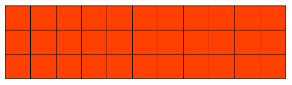
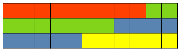
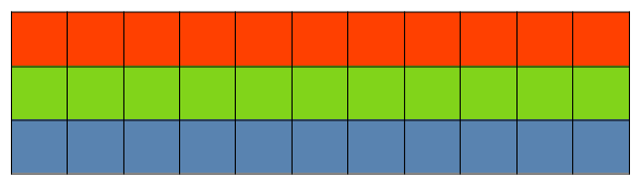
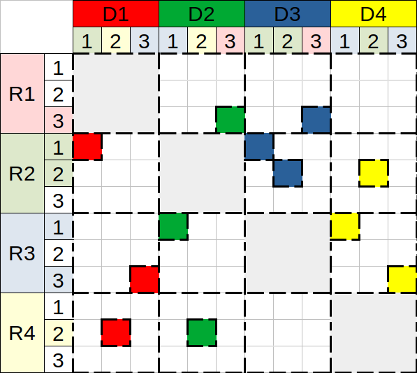
Denote the upper bound for consecutive cells-per-partition. Practically, the sketch can be viewed as a one-dimensional array of concatenated rows, where its partitions contain exactly cells each, except for the last partition containing the leftover cells. When , the entire sketch is mapped to a partition, as shown in Fig. 1(a), and hence, there are only covering nodes. With partitioning by (Fig. 1(b)) a data node is able to spread out its sketch uniformly across its covering nodes. Thus, a sketch row may appear on more than one partition. With partitioning by (Fig. 1(c)) the entire row (its first counter through the last one) is a member of a particular partition, implying that .
Partitioning example.
Figure 1 illustrates the three types of sketch partitioning and their impact on the ability to engage as much other nodes as possible. It reflects a system with data nodes, using distributed redundancy to tolerate any single failure, . Given the parameters , the sketch capacity is defined by rows and columns, i.e., CMS generates a matrix of counters. With partitioning by , the sketch can be divided into partitions, where the first 3 partitions contain 9 cells each, and the one contains the remaining 6 cells. However, with partitioning by , no more than 3 partitions can coexist.
5.2.2 Coverage Mapping
We now combine the sketch partitioning into distributed redundancy, and briefly describe three coverage mapping types, which slightly differ in their preferences regarding space-recovery trade-off. The mapping, or its generation algorithm, is given to a system, such that all the nodes are globally configured with the same mapping.
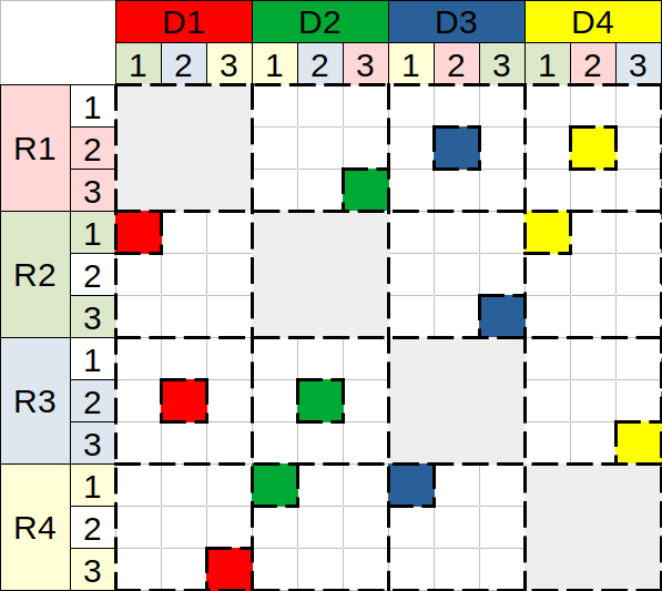
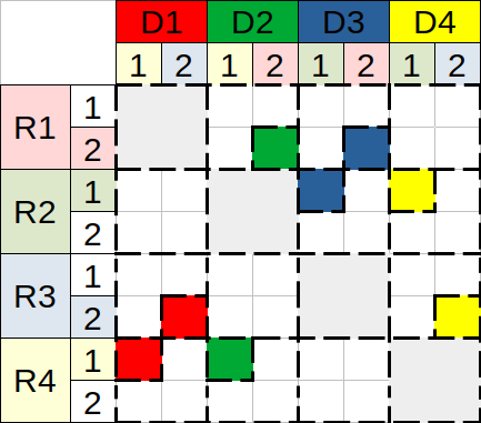
Figure 2 reflects a system with data nodes, using distributed redundancy to tolerate any single failure, . Hence, for such a system, and . The mapping is illustrated using a single coverage matrix, which can be divided into a series of partition-specific mappings, and respective matrices. The columns represent the partitioned data, denoted for a node , while the rows stand for redundant partitions a node covers. The redundant space of a node is therefore proportional to the number of partitions it actually covers, which are colored next to each . When a node fails, its partition-rows become invalid. To validate them back again and fully recover a node, we need to recover its data and reconstruct the redundancy it held prior to failure.
Mapping types.
We begin with maximal and aim to achieve balanced redundant space. Using the clique topology, a node covers some partitions of all other nodes, each of which covers a different partition of . The redundant vectors of the first mapping in Fig. 2(a) vary in the number of their non-zero coefficients (e.g., but ), implying that the overall redundant space is not minimal, indeed . However, this type is slightly better for recovery traffic, than space-oriented types, requiring only sketches to recover a failed node.
Towards space-oriented mapping, we define all (non-zero) redundant vectors to contain the same amount of non-zero coefficients. Minimal is achieved in Fig. 2(b), using six redundant partitions in total. However, they cannot be divided equally across the four nodes. As a result, the redundant space per node is imbalanced, implying slight variance in recovery traffic, . Such a mapping can be useful in heterogeneous setting, where the nodes differ in their capabilities (e.g., due to overlap period of storage replacement). Hence, delegating more work to the capable ones suits fairness design.
Towards balanced space-oriented mapping, we tune by reducing its value, and propose final mapping in Fig. 2(c), which consists of four redundant vectors, having exactly two non-zero coefficients each. Besides its space properties, this mapping requires exactly sketches to recover any of the failed nodes.
6 Periodic Updates
We examine sharing the redundant information upon regular time intervals, and assume that the maximum number of arrivals per time interval is bounded by a batch size .
The nodes operate in cycles, exchanging messages over reliable end-to-end communication service, i.e., the time interval encapsulates the retransmissions performed by the lower-level protocols we rely on. We assume timely delivery of messages, as well as that each node is equipped with incoming message queue having large enough memory to buffer all the messages that arrive during the cycle. In case a message from a certain data node fails to arrive on time, we consider this to be a crash failure, and initiate the recovery procedure of its sketch. If a data node has nothing to share, it sends the minimum message signalling that it is still alive. On each cycle, a redundant node reads all the incoming messages and updates its sum sketch accordingly. Let us note that in practice, when a message containing a sketch update is delivered at a redundant node, handling this message temporarily takes a corresponding extra space until the sketch data is consumed and its memory is freed.
6.1 Update policies
When , no delay is activated, and we update the redundant nodes on each item arrival. Otherwise, to maintain the redundancy, we consider the following two update policies:
Full Share policy.
With this policy, data nodes send their entire sketches causing the redundant nodes to reconstruct their sum sketches from scratch, e.g., to sum all the data sketches, which were delivered by the start of a cycle. Recall that each sketch counter is associated with a particular partition. Given a coverage mapping from 5.2.2, a data node encodes each partition by simply concatenating the relevant range of its sketch counters. To do so, the counters are tested for membership. Yet, with partitioning by , all the counters of a particular row are mapped to the same partition and hence, it’s enough to test only one of them, reducing the number of membership tests. Moreover, with partition, no membership testing is required at all, since all the counters are mapped together. When done encoding partitions, a data node constructs a message for each of its covering redundant nodes, consisting of only the partitions it covers. In such a manner, data nodes are able to send the bare minimum of copies for each counter.
We note that full share is essential for the recovery procedure of a failed sketch, which subtracts the non-failed counts from the overall sum. However, sending the entire sketch every time interval during the maintenance, over and over again, implies unnecessary communication overhead, especially if only few changes occurred. Moreover, a redundant node must wait to receive the updates from all data nodes that under its cover, before an older sum can be safely freed. To this end, as a communication-oriented solution, we consider sharing in an incremental manner only the changes, caused by the items that arrived during the cycle.
Incremental Share policy.
With this policy, a data node needs to encode the changes that occurred during the cycle. This can be done by either () recording each item arrival, () capturing the identifiers of the items that arrived and the number of times each of them arrived, or () recording the counters that have been changed and by how much. In options () and (), to reduce the space requirements, we consider capturing only the identifiers444In case of long identifiers, one can apply a cryptographic hash function to produce shorter fixed-length fingerprints. of arrived items. In options () and () we need counters, but these counters might be much smaller than the regular sketch counters, as they only need to count up to a batch size. Additional local data structure is required to host and manage the batch.
6.2 Framework API
We now introduce a generic framework for CMS, that besides its normal activity, supports batching, as shown in Algo. 2. Then, we examine some batch representations in more details.
Define to count the delayed items between the consecutive shares, . Initially, as well as after sharing the batch, counter is zeroed and batch representation is reset too. When an item arrives, in addition to the normal CMS execution, counter is incremented and an item is processed into a batch, where ’s recent value can be used as an index, e.g., in Buffer representations.
The general scheme for send procedures is provided in Algo. 3. Representations that record counters need to implement and functions, while others need to implement . When encoding rows of a fixed length, we can specify a row-width (actual number of elements) into a message’s header. However, when encoding variable-length rows, which is also the case when sketch is partitioned by cells, we need to encode these rows such that a redundant node can recognize the sketch row, each decoded element belongs to. For this purpose, besides the elements associated with a row, we first specify the number of elements to appear on that row. We call this metadata encoding.
6.3 Batch Representations
We examine several data structures to economically represent and encode a batch of changes. We consider two main categories – item-based vs counter-based data structures, each of which can be implemented as a Buffer or a Compact Hash Table. Table 2 lists the main aspects of their complexity, e.g., the extra local space they require, the amount of traffic they produce on each cycle, and the extra computation they imply, while omitting notation for space saving. For further evaluation, these are expressed using hyper-parameters. We then compare the representations to each other, and to the baseline option of a full share, as well.
- Buffer of Items.
-
The naïve approach for handling incremental shares is to record the arrived items in a local buffer, . Upon filling the buffer with at most items during the cycle, simply send the content to all the covering redundant nodes, as defined by coverage mapping. A receiving redundant node will then extract the identifiers and execute an update procedure against its sum sketch, recalculating the hash functions for each delivered item.
Buffer of Items is a simple and easy-to-implement, but also has some drawbacks:
-
Extra hash calculations must be performed by the redundant nodes on update.
-
All the buffered items must be sent to every covering redundant node, .
-
No room for privacy, since items’ identifiers are openly shared.
-
Different instances of a flow are handled independently of each other – duplicates.
To overcome these, we may () turn to counter-based representations, and/or () avoid duplicates through aggregation.
-
- Buffer of Counters.
-
Turning to counter-based representation, only a data node performs CMS hash calculations. The resulting indices are captured in a buffer of counters . For each counter, a data node knows exactly which redundant nodes cover it, so the bare minimum of copies can be sent. A receiving redundant node will then extract the indices and increment the corresponding counts of its sum sketch. As all the nodes are identically configured, we cannot guarantee that the privacy is protected with counters. Yet, it’s clearly better preserved than if sharing items.
- Hash Table of Flows.
-
tries to improve through duplicate avoidance, but it requires longer elements to additionally store the corresponding frequencies, using key-value pairs, as well as additional capacity due to the load threshold of a hash table.
- Hash Table of Counters.
-
Similarly, can be replaced by hash tables of counters, where is associated with a sketch row .
Hosting a batch.
Recall that within a stream of items, there are only flows (distinct items). Splitting the stream’s timeline by regular time intervals would result in cycles, each having associated batch. For ease of reference we assume the batches are full, i.e., contain items each. With incremental share we zoom into a given cycle.
Denote the number of flows that arrived during that particular cycle, and the number of modified sketch counters. Throughout the stream’s timeline, , but , since the same flow contributes to every batch it appears on. Denote the average frequency-per-flow within a given batch, then . Although the true values can be discovered in retrospect, but we need to decide on batch’s representation and allocate the memory in advance. To that end we could use some estimations on . For this purpose, we measure some statistics among different known large Internet traces.
6.4 Evaluating Compact Hash Table
In this paper, we evaluate the usage of compact hash tables through a comparison between and . We generally prioritize to reduce the communication traffic and avoid early transmissions, but space efficiency is also desired. To evaluate the traffic produced by these representations, we need to compare vs . We measured the traces using various batch sizes and hence, we consider the results as the range for any smaller Internet trace, e.g., within campus. The source code for measuring and generating the plots, as shown in Fig. 3 and Fig. 4, is now available at GitHub [6]. Given we further estimate the number of unique flows , and derive the initial capacity for buckets.
Over-allocation vs early transmission trade-off.
With low percentile we reduce the probability of early transmission, but the cost is space over-allocation. To choose the right for a given batch size , we look for the lowest percentile that holds: () and for communication traffic efficiency (colored in yellow), and () for space efficiency.
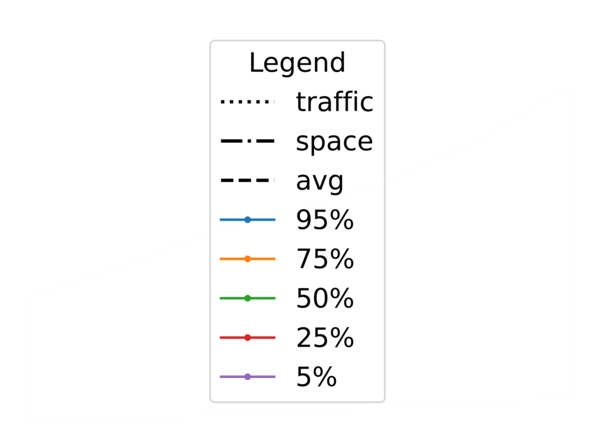
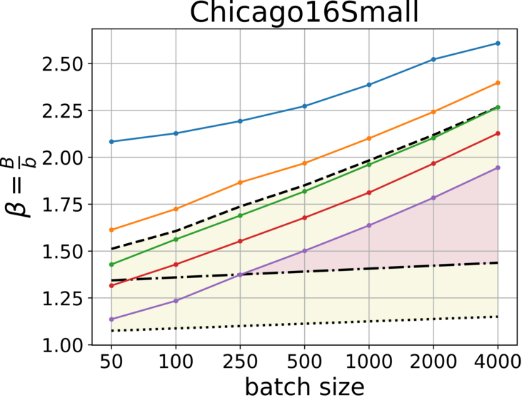
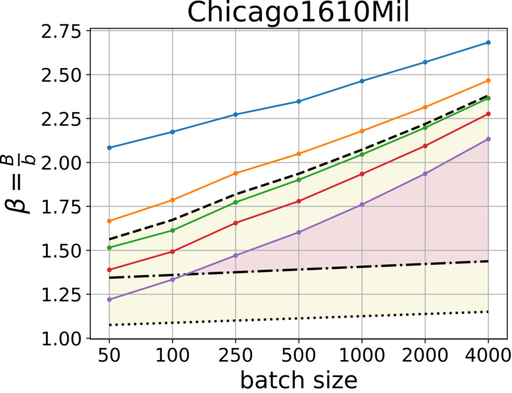
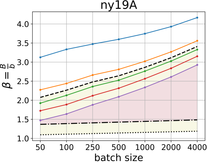
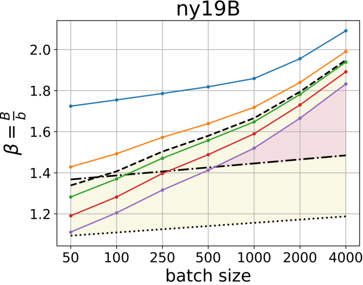
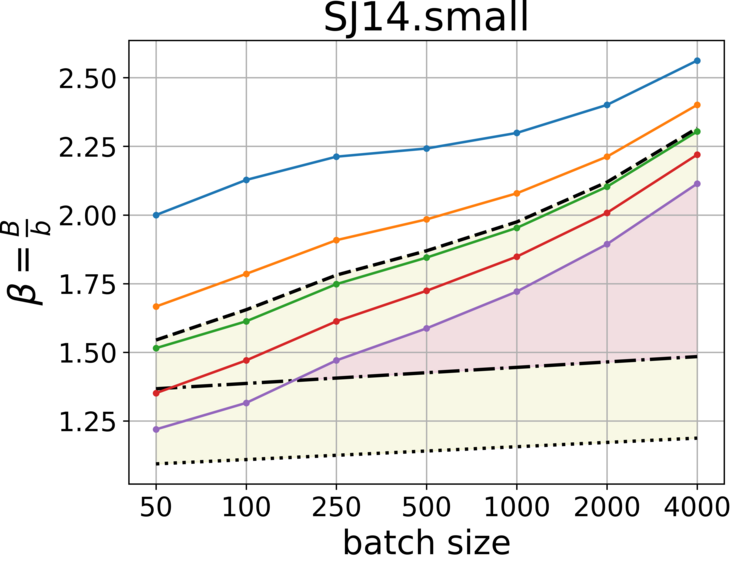
From the plots we learn additional approach to gain both space and traffic efficiency simultaneously (colored in magenta), by increasing the batch size. However, we need to keep in mind that upon recovery of a failed sketch, the batch size has a significant impact on the estimation error.
7 Conclusions
In this paper we have presented the motivation for recoverable sketches in a network environment, where each data node holds its own local sketch while the redundant nodes provide backup services for data nodes. Our distributed redundancy approach is based on the combination of these two roles, which can be implemented as independent services running on the same node. We introduced sketch partitioning into the model for load balancing, described how this parameter can be tuned, and provided different mappings to define the relations between the nodes.
We discovered an interesting imbalanced mapping, which can be useful in heterogeneous setting, and suit fairness design. An interesting direction for future work is to implement our design, and test the variety of settings in real-world datasets, exploring the potential of industry use.
References
- [1] Nikolas Askitis. Fast and compact hash tables for integer keys. In Proceedings of the Thirty-Second Australasian Conference on Computer Science - Volume 91, ACSC ’09, pages 113–122, Darlinghurst, Australia, January 2009. Australian Computer Society, Inc. URL: http://dl.acm.org/citation.cfm?id=1862675.
- [2] Ran Ben Basat, Xiaoqi Chen, Gil Einziger, Roy Friedman, and Yaron Kassner. Randomized admission policy for efficient top-k, frequency, and volume estimation. IEEE/ACM Transactions on Networking, 27(4):1432–1445, August 2019. doi:10.1109/TNET.2019.2918929.
- [3] Theophilus Benson, Ashok Anand, Aditya Akella, and Ming Zhang. Microte: fine grained traffic engineering for data centers. In Proceedings of the Seventh COnference on Emerging Networking EXperiments and Technologies, CoNEXT ’11, New York, NY, USA, 2011. Association for Computing Machinery. doi:10.1145/2079296.2079304.
- [4] Moses Charikar, Kevin Chen, and Martin Farach-Colton. Finding frequent items in data streams. Theoretical Computer Science, 312(1):3–15, January 2004. Automata, Languages and Programming. doi:10.1016/S0304-3975(03)00400-6.
- [5] Peter M. Chen, Edward K. Lee, Garth A. Gibson, Randy H. Katz, and David A. Patterson. Raid: High-performance, reliable secondary storage. ACM Computing Surveys, 26(2):145–185, June 1994. doi:10.1145/176979.176981.
- [6] Diana Cohen. Measuring average frequency of batched items in Internet traces, November 2024. URL: https://github.com/DianaCohenCS/measure-traces.
- [7] Saar Cohen and Yossi Matias. Spectral bloom filters. In Proceedings of the 2003 ACM SIGMOD International Conference on Management of Data, SIGMOD ’03, pages 241–252, New York, NY, USA, 2003. Association for Computing Machinery. doi:10.1145/872757.872787.
- [8] Graham Cormode and S. Muthukrishnan. An improved data stream summary: The count-min sketch and its applications. Journal of Algorithms, 55(1):58–75, April 2005. doi:10.1016/j.jalgor.2003.12.001.
- [9] Martin Dietzfelbinger and Christoph Weidling. Balanced allocation and dictionaries with tightly packed constant size bins. Theoretical Computer Science, 380(1):47–68, June 2007. Automata, Languages and Programming. doi:10.1016/j.tcs.2007.02.054.
- [10] Gero Dittmann and Andreas Herkersdorf. Network processor load balancing for high-speed links. In Proceedings of the 2002 International Symposium on Performance Evaluation of Computer and Telecommunication Systems, July 2002.
- [11] Java SE Documentation. Class hashmap. URL: https://docs.oracle.com/javase/8/docs/api/java/util/HashMap.html.
- [12] RabbitMQ Documentation. Batch publishing. URL: https://www.rabbitmq.com/docs/publishers#batch-publishing.
- [13] Shir Landau Feibish, Yehuda Afek, Anat Bremler-Barr, Edith Cohen, and Michal Shagam. Mitigating dns random subdomain ddos attacks by distinct heavy hitters sketches. In Proceedings of the Fifth ACM/IEEE Workshop on Hot Topics in Web Systems and Technologies, HotWeb ’17, New York, NY, USA, 2017. Association for Computing Machinery. doi:10.1145/3132465.3132474.
- [14] B. Mukherjee, L. T. Heberlein, and K. N. Levitt. Network intrusion detection. Netwrk. Mag. of Global Internetwkg., 8(3):26–41, May 1994. doi:10.1109/65.283931.
- [15] Rasmus Pagh and Flemming Friche Rodler. Cuckoo hashing. Journal of Algorithms, 51(2):122–144, May 2004. doi:10.1016/j.jalgor.2003.12.002.
- [16] Nicolas Le Scouarnec. Cuckoo++ hash tables: High-performance hash tables for networking applications, 2017. arXiv:1712.09624, doi:10.48550/arXiv.1712.09624.
- [17] W. Richard Stevens. TCP/IP illustrated (vol. 1): the protocols. Addison-Wesley Longman Publishing Co., Inc., USA, 1993. URL: http://dl.acm.org/citation.cfm?id=161724.