Near-Optimal Resilient Labeling Schemes

In Algorithm 1, the oracle first constructs a greedy $(2f+2,2f+1)$-ruling set $S$. For every node $v$, let $b(v)$ be a single bit indicating whether $v\in S$, and let $distS(v)$ be an $O(\log f)$-bit value which is the distance between $v$ and $S$.

The oracle then partitions the nodes into groups of size $\mathrm{\Theta }(f)$. To later allow the distributed algorithm to reconstruct the same groups, the oracle uses the same algorithm the nodes will later use, i.e., Algorithm 3. However, for the description in this section, any partitioning with the same guarantees would give the desired result in Theorem 3 below.

Finally, the oracle applies an error-correcting code to each index of the labels of all nodes in each group. The new label it assigns to each node $v$ is a concatenation of its $b(v)$ and $distS(v)$ values, along with the encoded label.

Different codes $𝙲$ result in different overheads of ${\mathrm{\ell }}^{\prime }$ compared to $\mathrm{\ell }$. A simple repetition code takes the string $\mathrm{𝚒𝚗𝚏𝚘}$ of length $s$ and repeats it for $s$ blocks to create the resulting codeword $𝚠=𝙲(\mathrm{𝚒𝚗𝚏𝚘})$, which is trivially decodable given any $s-1$ blocks erasures. Splitting $𝚠$ back to $s$ pieces implies that ${𝚠}_i$ equals $\mathrm{𝚒𝚗𝚏𝚘}$ for every node $v_i$ in the group. Taking $f=F$, this results in ${\mathrm{\ell }}^{\prime }=1+O(\log f)+s\cdot \mathrm{\ell }=O(\log F)+s\cdot \mathrm{\ell }$. Since the group size $s$ is always $\mathrm{\Theta }(f)=\mathrm{\Theta }(F)$, we get a multiplicative overhead of $O(F)$ and an additive overhead of $O(\log F)$. To reduce the multiplicative overhead to $O(1)$, we use a code with better parameters. Formally, a binary code $𝙲$ maps strings of $k$ bits into strings of $N$ bits called codewords. The ratio $\rho =N/k$ is the code’s rate. The relative distance, $\delta$, ensures the Hamming distance (number of indices where the strings differ) between any two codewords is at most $\delta N$. Such a code can correct $\delta N-1$ erasures.

Given the bound $F$ on the number of label erasures, we need to choose a value of $f$ to work with. Then, given a group of size $s$ such that $f+1\le s\le 3f+1$, we need to choose values for $\rho$ and $M$ that determine the code ${𝙲}_M$. We set these parameters as follows. We let $f=80F$, and for every such $s$ we choose $\rho =1/4$. To choose $M$, notice that Lemma 2 gives that for any $M>0$, the number of bits we can encode is $k_M={\rho }_M{N}_M$. We choose the smallest $M$ such that $k_M$ is at least $s$.

The next theorem proves that the overhead for the number of bits held by each node per coded bit is constant and that, given the coded blocks,it is possible to decode the original string of bits if up to $F$ blocks are erased. The proof is presented in Appendix A.

For later use by the distributed algorithm in our resilient labeling scheme, we denote by $decode(v,\{(u,𝚠(u))\mid u\in Group(v)\})$ the function that takes as input a node $v$ and the values $𝚠(u)$ for all the nodes $u$ in $Group(v)$ (along with their IDs so that they can be ordered correctly) and produces the bit of $v$ in the string $𝚛$ which was encoded into $𝚠$, by Theorem 3.

In Algorithm 2, nodes restore a greedy ruling set $S$ as follows. Before the algorithm starts, each non-faulty node $w$ sets its value $b(w)$ to the first bit of its label. At the beginning of the algorithm, non-faulty nodes in $S$ broadcast a bit “1” for $2f+1$ rounds. Here, every node that receives a bit “1” during these rounds forwards it to all of its neighbors. Faulty nodes $u$ that receive a bit during these rounds sets $b(u)=0$, as this indicates that $u\in B_{2f+1}(v)$ for some such $v\in S$ and thus $u\notin S$.

Next, each faulty node propagates its ID through a distance of $2f+1$. Faulty nodes $u$ that do not receive any other ID set $b(u)=1$, as this means no other faulty nodes are in $B_{2f+1}(u)$ and thus $u\in S$.

Now, every remaining faulty node $u$ propagate a message of the form $ID(u)\circ dist$ through a distance of $f+1$, where $dist$ starts at 0 and is increased by 1 by each node along the way, corresponding to the length of the path. For each node $w$, let $dis{t}_u(w)$ be the smallest $dist$ value received for $u$, representing the actual distance between $w$ and $u$.

Each node $w\in B_{f+1}(u)$ receives the message and checks if it is possible that $u\in S$ by verifying whether $distS(w)=dis{t}_u(w)$. If this equality does not hold, $w$ propagates a message with $ID(u)$ through a distance of $f+1$. Since $dist(w,u)\le f+1$, if $u\in S$, then $distS(w)=dis{t}_u(w)$. If $w$ propagates $ID(u)$, then this is not the case, so when $u$ receives its own ID, it can conclude that it is not in $S$ and sets $b(u)=0$.

Now, we are left with faulty nodes $v\in S$ and faulty nodes $u\notin S$. We will prove that $u$ is an alternative node for a faulty node $v\in S$. Thus, every faulty node $v\in S$ must have the lowest ID among faulty nodes in $B_{f+1}(v)$ and can deduce that it is in $S$ and set $b(v)=1$. Similarly, every faulty node $u\notin S$ must have a faulty node $v\in S$ within $B_{f+1}(u)$ such that , allowing $u$ to deduce it is not in $S$ and set $b(u)=0$.

Following is the formal algorithm and proof.

To prove that the algorithm restores the set $S$, we prove that every node $w\in V$ holds $b(w)$ at the end of Algorithm 2, such that $\{w\mid b(w)=1\}=S$. By Step 2, this holds for all non-faulty nodes, so it remains to prove it for faulty nodes. In what follows, we go over each step in the algorithm where nodes may set their output (Steps 2,2,2, and 2), and we show that any node which sets its output during that step does so correctly.

In Step 2, every non-faulty node $v\in S$ broadcasts a bit “1” for $2f+1$ rounds. By the definition of a $(2f+2,2f+1)$-ruling set, every two nodes $v^{\prime },v^{\prime \prime }\in S$ satisfy that $dist(v^{\prime },v^{\prime \prime })\ge 2f+2$. Thus, if a faulty node $u$ receives a bit “1” from $v\in S$ during these $2f+1$ rounds, it implies that $u\in B_{f+1}(v)$. Hence, $u\notin S$ since $v\in S$. So, for any node $u$ that sets $b(u)=0$ in Step 2, its output is correct.

Afterwards, in Step 2, each faulty node propagates a message with its ID through a distance of $2f+1$. Every faulty node $u$ that does not receive any other ID during these rounds and did not receive a “1” during Step 2 sets $b(u)=1$, because this implies that there is no other faulty node in $B_{2f+1}(u)$ and hence it must hold that $u\in S$. So, it is correct that $u$ sets $b(u)=1$ in Step 2.

Then, in Step 2, every node $u$ that is still faulty propagates a message of the form $ID(u)\circ dist$ through a distance of $f+1$, where $dist$ starts at $0$ and is increased by $1$ before the message is propagated further. This corresponds to the length of the path that this message traverses. Every node $w\in B_{f+1}(u)$ receives the above message and checks if it is possible that $u\in S$ by verifying whether $distS(w)=dis{t}_u(w)$. We denote by $dist(u)$ the value of $dist$ from the message $ID(u)\circ dist$ that $w$ receives. If equality does not hold, then $w$ propagates a message with $ID(u)$ through a distance of $f+1$. Since $dist(u,w)\le f+1$, if $u\in S$, then for every other node $v^{\prime }\in S$ such that $dist(w,v^{\prime })\le f+1$, it holds that $2f+2\le dist(u,v^{\prime })\le dist(u,w)+dist(w,v^{\prime })\le f+1+dist(w,v^{\prime })$. Thus, $dist(w,v^{\prime })\ge f+1$, and since $distS(w)={\min }_{v\in S}\{dist(q,v)\}$ we have $distS(w)=dis{t}_u(w)$. But if $w$ propagates $ID(u)$, then this is not the case, so $u\notin S$. Thus, it is correct that $u$ sets $b(u)=0$ in Step 2.

First we prove that every node $u$ that is still faulty at the beginning of this step and every node $v\in X(u)$ are alternative nodes. By definition of alternative nodes, we need to prove that $dist(u,v)\le f$ and that $v$ and $u$ have at most $f-2$ nodes $w\in B_{f+1}(v)\cup B_{f+1}(u)$ with $dist(u,w)\ne dist(v,w)$.

First, since $v\in X(u)$, it must be that $dist(u,v)\le f$. Second, we prove that $v$ and $u$ have at most $f-2$ nodes $t\in B_{f+1}(v)\cup B_{f+1}(u)$ with $dist(u,t)\ne dist(v,t)$. Assume, towards a contradiction, that there are at least $f-1$ nodes $t\in B_{f+1}(v)\cup B_{f+1}(u)$ with $dist(v,t)\ne dist(u,t)$. Since $u$ is still faulty in Step 2, there are at most $f-2$ nodes $q\ne u,v$ in $B_{f+1}(u)$ with $dist(u,q)\ne dist(v,q)$, because otherwise $u$ would receive a message with $ID(u)$ from such a non-faulty node during Step 2 and would set $b(u)=0$ in Step 2. Therefore, there exists a node $s\in B_{f+1}(v)\setminus B_{f+1}(u)$ that is still faulty in Step 2. We consider two cases, obtaining a contradiction in both, and conclude that the assumption is incorrect. Thus, $v$ and $u$ have at most $f-2$ nodes $t\in B_{f+1}(v)\cup B_{f+1}(u)$ with $dist(u,t)\ne dist(v,t)$.

An illustration of this case is presented in Figure 1.

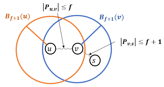
In this case, every node $t\ne u,v$ on $P_{v,u}$ satisfies that $dist(u,t)\ne dist(v,t)$, except at most one node $a$ (such a node $a$ exists if $dist(u,v)$ is even and $a$ is exactly in the middle of $P_{v,u}$). Additionally, every node $t$ on $P_{v,s}$ satisfies that $dist(t,v)\ne dist(t,u)$, as otherwise $dist(u,s)\le dist(u,t)+dist(t,s)=dist(v,t)+dist(t,s)=dist(v,s)\le f+1$, which contradicts the assumption that $dist(u,s)\ge f+2$. Denote by $P^{\prime }$ the path $P_{u,v}\circ P_{v,s}$ at a distance of at most $f+1$ from $u$. There are $f$ nodes on $P^{\prime }$ that are neither $u$ nor $v$. Additionally, excluding the node $a$, we have $f-1$ nodes $q$ on $P^{\prime }$ with $dist(v,q)\ne dist(u,q)$, and they are all in $B_{f+1}(u)$. This contradicts the assumption that there are at most $f-2$ such nodes. Therefore, this case in not possible.

An illustration of this case is presented in Figure 2.

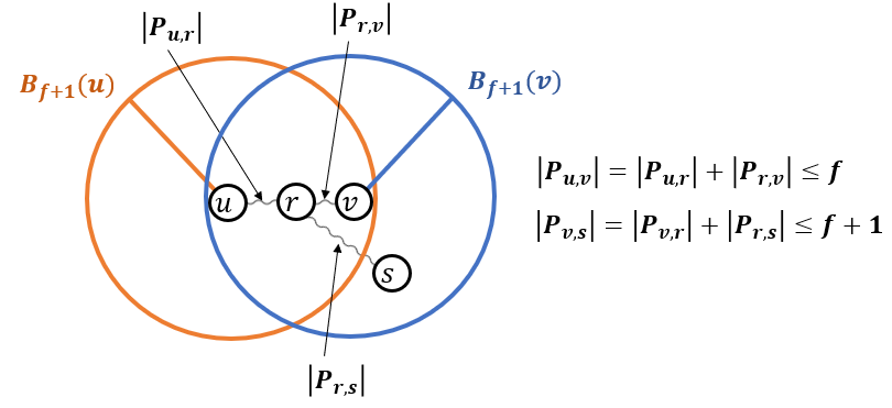
We consider $r$ to be the closest node to $u$ in $P_{v,u}\cap P_{v,s}$. In this case, every node $t\ne u,v$ on $P_{v,u}$ satisfies that $dist(u,t)\ne dist(v,t)$, except at most one node $a$, as we proved in the previous case. Therefore, it is also correct for $P_{u,r}$. Additionally, every node $t$ on $P_{r,s}$ satisfies that $dist(t,v)\ne dist(t,u)$, as otherwise $dist(u,s)\le dist(u,t)+dist(t,s)=dist(v,t)+dist(t,s)=dist(v,s)\le f+1$, contradicting the assumption that $dist(u,s)\ge f+2$.

Denote by $P^{\prime }$ the path $P_{u,r}\circ P_{r,s}$ at a distance of at most $f+1$ from $u$. There are $f+1$ nodes on $P^{\prime }$ that are not $u$. Additionally, excluding the node $a$, we have $f$ nodes $q$ on $P^{\prime }$ with $dist(v,q)\ne dist(u,q)$, and they are all in $B_{f+1}(u)$. This contradicts the assumption that there are at most $f-2$ such nodes. Therefore, this case in not possible.
This completes the proof that every node $u$ that is still faulty at the beginning of this step and every node $v\in X(u)$ are alternative nodes.

Now, we prove that if $u$ sets $b(u)=0$ in this step, then it satisfies that $u\notin S$. In this case, since $u$ sets $b(u)=0$, there exists a node $v\in X(u)$ with . Since $v$ is an alternative node for $u$ with , it follows that $u\notin S$ by Lemma 6.

Finally, we prove that every faulty node $u$ that sets $b(u)=1$ satisfies that $u\in S$. By the definition of a $(2f+2,2f+1)$-ruling set, there exists a node $v\in S$ such that $dist(u,v)\le 2f+1$ (which may be $u$ itself). We claim that $v\in B_f(u)$. Assume otherwise, i.e., that $dist(u,v)\ge f+1$. Notice that $v,u$ have at least $|P_{v,u}|-2$ nodes $j$ with $dist(v,j)\ne dist(u,j)$ on $P_{v,u}$, since there are $|P_{v,u}|-1$ nodes $j\ne u,v$ on $P_{v,u}$, and at most one of them has $dist(v,j)=dist(u,j)$ (such a node $j$ exists if $dist(u,v)$ is even and $j$ is exactly in the middle of $P_{v,u}$). Therefore, if $dist(u,v)\ge f+1$, consider nodes on the path $P_{u,v}$ that are at a distance of at most $f+1$ from $u$. There are at least $f-1$ such nodes $j\ne u,v$ with $dist(u,j)\ne dist(v,j)$, and so at least one of them is not faulty, which would lead to $u$ setting $b(u)=0$ in Step 2. But, $u$ is faulty at the beginning of Step 2, which leads to a contradiction.

Thus, $v\in B_f(u)$. Additionally, $v\in X(u)$ because in Step 2, $u$ is still faulty, and therefore, in Step 2, $u$ does not set $b(u)=0$, so $v$ must also still be faulty in Step 2. Since $dist(u,v)\le 2f+1$ and $v$ is still faulty in Step 2, $u$ receives a message with $ID(v)$ in Step 2. Note that if $v$ is not faulty in Step 2, then either it is non-faulty to begin with, in which case $u$ would have already set $b(u)=0$ in Step 2, or $v$ sets $b(v)=1$ in Step 2. The latter is impossible because $dist(u,v)\le 2f+1$ and $u$ is still faulty in Step 2. Thus, $v$ is still faulty in Step 2, which means that $v$ would receive a message from $u$ in Step 2 and not set $b(v)=1$ in Step 2. Thus, $v$ is also still faulty in Step 2, and since $dist(u,v)\le f$, then $v\in X(u)$.

Thus, since $u$ sets $b(u)=1$, every node $w\in X(u)$ satisfies $ID(u)\le ID(w)$. Since, $w\in X(u)$, then as we proved, $w$ is an alternative node for $u$. By Lemma 6, this implies that $w$ cannot be in $S$. Since $v\in X(u)\cap S$, it must hold that $v=u$. Thus $u\in S$, as needed.

This completes the proof that, at the end of Algorithm 2, we set $b(w)$ for every node $w\in V$ correctly, satisfying $\{w|b(w)=1\}=S$. Finally, we sum the number of rounds the algorithm takes. In every broadcast in the algorithm, we have at most $f$ different messages (each of which fits in $O(\log n)$ bits). Moreover, a node passes such a message only once. Thus, each broadcast takes $O(f)$ rounds. Since there are only a constant number of steps with such broadcasts, the algorithm completes in $O(f)$ rounds. $◀$

Algorithm 3 constructs the required partition as follows. Initially, each node $v\in S$ computes a BFS tree to depth $2f+1$ by propagating its ID. Nodes that receive multiple root IDs choose the smallest and use that tree only. The rest of the algorithm operates within each tree independently.

Within each tree, each node $u$ divides the nodes in its subtree into groups of size $f+1\le s\le 3f+1$, with a remainder of up to $f$ nodes. This remaining number is sent to its parent $parent(u)$, who handles dividing the remainders of its children similarly. The $\mathrm{𝙲𝚘𝚖𝚙𝚞𝚝𝚎𝙶𝚛𝚘𝚞𝚙𝚜}(u)$ procedure sorts $u$’s children by increasing IDs, appends itself, and then forms groups by summing the remaining values of its children. Once a group reaches the desired size, a new group starts from the next child. Each child receives its group ID from $u$. When a node receives its group allocation, it may need to inform some of its children to ensure that remaining nodes from its subtree join this group as well. This is handled by the $\mathrm{𝚁𝚎𝚕𝚊𝚢𝙶𝚛𝚘𝚞𝚙𝚜}(u)$ procedure, in which node $u$ relays the group ID. During this process, $u$ also sets the local variable $H_u$ which is used for constructing low-congestion shortcuts for communication among the nodes of each group. Finally, if there is a small remainder at the root $v$, the root appends these nodes to one of the groups created in $\mathrm{𝙲𝚘𝚖𝚙𝚞𝚝𝚎𝙶𝚛𝚘𝚞𝚙𝚜}(v)$ or, if no such group was constructed by $v$, it appends them to a group with the closest node from this group to $v$. This is done by $v$ obtaining the required group ID and relaying it to the relevant remaining nodes.

Following is the formal algorithm and proof.

References

- [1] Ittai Abraham, Shiri Chechik, and Cyril Gavoille. Fully dynamic approximate distance oracles for planar graphs via forbidden-set distance labels. In Proceedings of the forty-fourth annual ACM symposium on Theory of computing, pages 1199–1218, 2012. doi:10.1145/2213977.2214084.
- [2] Stephen Alstrup, Cyril Gavoille, Haim Kaplan, and Theis Rauhe. Nearest common ancestors: a survey and a new distributed algorithm. In Proceedings of the fourteenth annual ACM symposium on Parallel algorithms and architectures, pages 258–264, 2002. doi:10.1145/564870.564914.
- [3] Yagel Ashkenazi, Ran Gelles, and Amir Leshem. Noisy beeping networks. Inf. Comput., 289(Part):104925, 2022. doi:10.1016/J.IC.2022.104925.
- [4] Alkida Balliu, Sebastian Brandt, Fabian Kuhn, and Dennis Olivetti. Distributed -coloring plays hide-and-seek. In Stefano Leonardi and Anupam Gupta, editors, STOC ’22: 54th Annual ACM SIGACT Symposium on Theory of Computing, Rome, Italy, June 20 - 24, 2022, pages 464–477. ACM, 2022. doi:10.1145/3519935.3520027.
- [5] Aviv Bar-Natan, Panagiotis Charalampopoulos, Paweł Gawrychowski, Shay Mozes, and Oren Weimann. Fault-tolerant distance labeling for planar graphs. Theoretical Computer Science, 918:48–59, 2022. doi:10.1016/J.TCS.2022.03.020.
- [6] Mor Baruch, Pierre Fraigniaud, and Boaz Patt-Shamir. Randomized proof-labeling schemes. In Proceedings of the 2015 ACM Symposium on Principles of Distributed Computing, pages 315–324, 2015. doi:10.1145/2767386.2767421.
- [7] Aviv Bick, Gillat Kol, and Rotem Oshman. Distributed zero-knowledge proofs over networks. In Proceedings of the 2022 Annual ACM-SIAM Symposium on Discrete Algorithms (SODA), pages 2426–2458. SIAM, 2022. doi:10.1137/1.9781611977073.97.
- [8] Keren Censor-Hillel, Ami Paz, and Mor Perry. Approximate proof-labeling schemes. Theor. Comput. Sci., 811:112–124, 2020. doi:10.1016/J.TCS.2018.08.020.
- [9] Michal Dory and Merav Parter. Fault-tolerant labeling and compact routing schemes. In Proceedings of the 2021 ACM Symposium on Principles of Distributed Computing, pages 445–455, 2021. doi:10.1145/3465084.3467929.
- [10] Yuval Emek and Yuval Gil. Twenty-two new approximate proof labeling schemes. In Hagit Attiya, editor, 34th International Symposium on Distributed Computing, DISC 2020, October 12-16, 2020, Virtual Conference, volume 179 of LIPIcs, pages 20:1–20:14. Schloss Dagstuhl – Leibniz-Zentrum für Informatik, 2020. doi:10.4230/LIPICS.DISC.2020.20.
- [11] Yuval Emek, Yuval Gil, and Shay Kutten. Locally Restricted Proof Labeling Schemes. In Christian Scheideler, editor, 36th International Symposium on Distributed Computing (DISC 2022), volume 246 of LIPIcs, pages 20:1–20:22, Dagstuhl, Germany, 2022. Schloss Dagstuhl – Leibniz-Zentrum für Informatik. doi:10.4230/LIPIcs.DISC.2022.20.
- [12] Salwa Faour, Mohsen Ghaffari, Christoph Grunau, Fabian Kuhn, and Václav Rozhoň. Local distributed rounding: Generalized to mis, matching, set cover, and beyond. In Proceedings of the 2023 Annual ACM-SIAM Symposium on Discrete Algorithms (SODA), pages 4409–4447. SIAM, 2023. doi:10.1137/1.9781611977554.CH168.
- [13] Laurent Feuilloley. Introduction to local certification. Discrete Mathematics & Theoretical Computer Science, 23(Distributed Computing and Networking), 2021. doi:10.46298/DMTCS.6280.
- [14] Laurent Feuilloley and Pierre Fraigniaud. Error-sensitive proof-labeling schemes. J. Parallel Distributed Comput., 166:149–165, 2022. doi:10.1016/J.JPDC.2022.04.015.
- [15] Laurent Feuilloley, Pierre Fraigniaud, Juho Hirvonen, Ami Paz, and Mor Perry. Redundancy in distributed proofs. Distributed Computing, 34:113–132, 2021. doi:10.1007/S00446-020-00386-Z.
- [16] Orr Fischer, Rotem Oshman, and Dana Shamir. Explicit space-time tradeoffs for proof labeling schemes in graphs with small separators. In Quentin Bramas, Vincent Gramoli, and Alessia Milani, editors, 25th International Conference on Principles of Distributed Systems (OPODIS 2021), LIPIcs, pages 21:1–21:22, Dagstuhl, Germany, 2022. Schloss Dagstuhl – Leibniz-Zentrum für Informatik, Schloss Dagstuhl – Leibniz-Zentrum für Informatik. doi:10.4230/LIPIcs.OPODIS.2021.21.
- [17] Pierre Fraigniaud, Cyril Gavoille, David Ilcinkas, and Andrzej Pelc. Distributed computing with advice: information sensitivity of graph coloring. Distributed Computing, 21:395–403, 2009. doi:10.1007/S00446-008-0076-Y.
- [18] Pierre Fraigniaud, David Ilcinkas, and Andrzej Pelc. Communication algorithms with advice. Journal of Computer and System Sciences, 76(3-4):222–232, 2010. doi:10.1016/J.JCSS.2009.07.002.
- [19] Pierre Fraigniaud, Amos Korman, and Emmanuelle Lebhar. Local mst computation with short advice. In Proceedings of the nineteenth annual ACM symposium on Parallel algorithms and architectures, pages 154–160, 2007. doi:10.1145/1248377.1248402.
- [20] Emanuele G Fusco and Andrzej Pelc. Trade-offs between the size of advice and broadcasting time in trees. In Proceedings of the twentieth annual symposium on Parallelism in algorithms and architectures, pages 77–84, 2008. doi:10.1145/1378533.1378545.
- [21] Cyril Gavoille and David Peleg. Compact and localized distributed data structures. Distributed Computing, 16:111–120, 2003. doi:10.1007/S00446-002-0073-5.
- [22] Cyril Gavoille, David Peleg, Stéphane Pérennes, and Ran Raz. Distance labeling in graphs. Journal of algorithms, 53(1):85–112, 2004. doi:10.1016/J.JALGOR.2004.05.002.
- [23] Paweł Gawrychowski, Fabian Kuhn, Jakub Łopuszański, Konstantinos Panagiotou, and Pascal Su. Labeling schemes for nearest common ancestors through minor-universal trees. In Proceedings of the Twenty-Ninth Annual ACM-SIAM Symposium on Discrete Algorithms, pages 2604–2619. SIAM, 2018.
- [24] Mohsen Ghaffari and Bernhard Haeupler. Distributed algorithms for planar networks ii: Low-congestion shortcuts, mst, and min-cut. In Proceedings of the twenty-seventh annual ACM-SIAM symposium on Discrete algorithms, pages 202–219. SIAM, 2016. doi:10.1137/1.9781611974331.CH16.
- [25] Mika Göös and Jukka Suomela. Locally checkable proofs. In Proceedings of the 30th annual ACM SIGACT-SIGOPS symposium on Principles of distributed computing, pages 159–168, 2011. doi:10.1145/1993806.1993829.
- [26] Mika Göös and Jukka Suomela. Locally checkable proofs in distributed computing. Theory of Computing, 12(1):1–33, 2016. doi:10.4086/TOC.2016.V012A019.
- [27] Rani Izsak and Zeev Nutov. A note on labeling schemes for graph connectivity. Information processing letters, 112(1-2):39–43, 2012. doi:10.1016/J.IPL.2011.10.001.
- [28] Taisuke Izumi, Yuval Emek, Tadashi Wadayama, and Toshimitsu Masuzawa. Deterministic fault-tolerant connectivity labeling scheme. In Proceedings of the 2023 ACM Symposium on Principles of Distributed Computing, pages 190–199, 2023. doi:10.1145/3583668.3594584.
- [29] Jørn Justesen. Class of constructive asymptotically good algebraic codes. IEEE Transactions on information theory, 18(5):652–656, 1972. doi:10.1109/TIT.1972.1054893.
- [30] Michal Katz, Nir A Katz, Amos Korman, and David Peleg. Labeling schemes for flow and connectivity. SIAM Journal on Computing, 34(1):23–40, 2004. doi:10.1137/S0097539703433912.
- [31] Gillat Kol, Rotem Oshman, and Raghuvansh R Saxena. Interactive distributed proofs. In Proceedings of the 2018 ACM Symposium on Principles of Distributed Computing, pages 255–264, 2018. URL: https://dl.acm.org/citation.cfm?id=3212771.
- [32] Amos Korman. Labeling schemes for vertex connectivity. ACM Transactions on Algorithms (TALG), 6(2):1–10, 2010. doi:10.1145/1721837.1721855.
- [33] Amos Korman and Shay Kutten. Distributed verification of minimum spanning trees. In Proceedings of the twenty-fifth annual ACM symposium on Principles of distributed computing, pages 26–34, 2006. doi:10.1145/1146381.1146389.
- [34] Amos Korman and Shay Kutten. On distributed verification. In Distributed Computing and Networking: 8th International Conference, ICDCN 2006, Guwahati, India, December 27-30, 2006. Proceedings 8, pages 100–114. Springer, 2006. doi:10.1007/11947950_12.
- [35] Amos Korman, Shay Kutten, and David Peleg. Proof labeling schemes. Distributed Comput., 22(4):215–233, 2010. doi:10.1007/S00446-010-0095-3.
- [36] Nathan Linial. Locality in distributed graph algorithms. SIAM Journal on computing, 21(1):193–201, 1992. doi:10.1137/0221015.
- [37] Rafail Ostrovsky, Mor Perry, and Will Rosenbaum. Space-time tradeoffs for distributed verification. In Shantanu Das and Sébastien Tixeuil, editors, Structural Information and Communication Complexity - 24th International Colloquium, SIROCCO 2017, Porquerolles, France, June 19-22, 2017, Revised Selected Papers, volume 10641 of Lecture Notes in Computer Science, pages 53–70. Springer, 2017. doi:10.1007/978-3-319-72050-0_4.
- [38] Merav Parter and Asaf Petruschka. Õptimal dual vertex failure connectivity labels. In Christian Scheideler, editor, 36th International Symposium on Distributed Computing, DISC 2022, October 25-27, 2022, Augusta, Georgia, USA, volume 246 of LIPIcs, pages 32:1–32:19. Schloss Dagstuhl – Leibniz-Zentrum für Informatik, 2022. doi:10.4230/LIPICS.DISC.2022.32.
- [39] Merav Parter, Asaf Petruschka, and Seth Pettie. Connectivity labeling for multiple vertex failures. arXiv preprint, 2023. doi:10.48550/arXiv.2307.06276.
- [40] Boaz Patt-Shamir and Mor Perry. Proof-labeling schemes: Broadcast, unicast and in between. In International Symposium on Stabilization, Safety, and Security of Distributed Systems, pages 1–17. Springer, 2017. doi:10.1007/978-3-319-69084-1_1.
- [41] David Peleg. Proximity-preserving labeling schemes. Journal of Graph Theory, 33(3):167–176, 2000. doi:10.1002/(SICI)1097-0118(200003)33:3\%3C167::AID-JGT7\%3E3.0.CO;2-5.
Appendix A Missing Proofs
A.1 Proof of Theorem 3
In order to prove this theorem, we need the following claim on .
Claim 10.
For every , it holds that .
Proof of Claim 10.
For every , the value of is defined as , and so we have for :
where the last inequality follows since and thus .
We now prove the aforementioned properties of the code implied by our choice of parameters using a very crude analysis of the constants, which is sufficient for our needs.
Proof of Theorem 3.
Since is the smallest such that , we have that , or in other words, . We prove in Claim 10 above that is at most . Combining these two with the fact that , gives that
where the last inequality follows since . This gives that is at most . To encode, we take the bits and pad them with zeros concatenated at their end. We get bits that are split among the nodes, so now the number of bits that each node has is at most . We know that and that is at most , so each node holds at most bits. This proves Item (1).
To prove Item (2), note that the code has a relative distance . The code can fix up to erasures, which is more than a fraction of . Since and the number of blocks is at least (which is at least ), any erasure of blocks erases at most a fraction of the blocks. Some blocks may be of size and others of size , which may differ by 1 and the larger blocks may get erased. However, even if we denote and assume , then in the worst case, the fraction of bit erasures caused by block erasures is at most , which is at most (since ). Thus, this may erase at most a fraction of bits of . Because the code can fix up to a fraction of erasures, we can decode , obtaining Item (2) as needed.
A.2 Proof of Lemma 6
Proof of Lemma 6.
Let and be alternative nodes, and let . We claim that if and only if . This implies that if then is a -ruling set. In particular, this means that apart from , the node does not have a node within distance at most from it. Therefore, cannot be smaller than , since otherwise the greedy algorithm would reach before when iterating over the nodes and would inserted into .
To prove that if and only if , we assume that and prove that . The proof for the other direction is symmetric. Assume towards a contradiction that it is not the case, so . Thus, using the triangle inequality we have
where the last inequality follows from the definition of as alternative nodes. Thus, . Assume towards a contradiction that there is a node on such that . Since is on then . Therefore,
This contradicts the assumption that . Thus, every node on satisfies .
Because , there are at least nodes on such that , and at least of them are at a distance of at most from . Thus, is not an alternative node for , contradicting the assumption. Therefore, .
A.3 Proof of Theorem 8
Proof of Theorem 8.
Since is a -ruling set, every node has a node within distance of at most from it. Thus, belongs to exactly one tree, and in the BFS in Step 3 in the algorithm, the node chooses one node to be its leader. Let be the tree rooted at .
The BFS tree of every node satisfies that .
For every node , there are at least nodes within distance from it (including itself), since the graph is connected. These nodes cannot be within distance from any other node , and thus they join the BFS tree . This proves that for all trees. In particular, there exists a partition of the nodes in into groups of sizes at least .
The algorithm obtains a partitioning of the nodes in every tree into groups with sizes ranging from to .
Fix and consider only nodes in . First, we prove that all groups created until the end of Step 3 are of size ranging from to . Let . In Step 3, the node runs the procedure . During the procedure, when creating a group, the node starts with the first child in and adds children according to until the counter of their values is at least . For a group that starts with child and ends with child , in Step 3 the node sends this group’s identifier to every child for which . Then, each sends in in Step 3 this group identifier to all its children for which it did not assign a group yet during the procedure , and its children relay this identifier in the same manner. Thus, the value of is the size of the group, and so this size is at least .
Notice that if is at most , when adding of some child , we get that the updated is at most (any value is always at most , as otherwise would form a group from these at least nodes). A special case is when a root of a subtree adds itself to a group it created, and then is at most . Therefore, since the size of a group is the value of , then the size of a group ranges from to .
This proves that all groups created until the end of Step 3 are of size ranging from to , but there still could be some values that needs to handle whose sum is . For every node , an ancestor of handles these values. But, the algorithm for the root in this case differs, as it has no ancestors. Steps 3-3 provide the root with a group ID to which it adds its remainder, so the size of that group may become at most . Thus, all the group sizes range from to .
Notice that since every node belongs to exactly one group, then all the groups are disjoint.
For each edge , the number of subgraphs containing is at most .
An edge is inserted into if sends the group identifier to and this happens only if sends to in Step 3. There are two cases. The first is that assigns a group during the steps of creating groups. Thus, does not assign another group in this or later steps. Therefore, in this case, the edge is inserted into only one set of . The same argument applies if the edge is inserted into during the steps of relaying group IDs.
The second case is that receives from its parent during the steps of handling the root remainder. Then, the root satisfies that . Thus, according to the algorithm, it assigns additional nodes to an existing group. Therefore, can be inserted into at most one additional group. Overall, there are at most two groups for which assigns to .
The diameter of the subgraph is at most .
Consider two cases, based on whether the group contains the root or not.
Case 1: Let be a group which does not contain the root , and let be the node that builds during . Since the group identifier is the ID of the first child in the group, there can be only a single that creates a group with this ID, and only nodes in the subtree of can belong to it.
Let . In Step 3, sends to and inserts the edge into . Additionally, if , then also receives from its parent and sets in Step 3 of procedure . This process continues until we reach a node which is a child of . Since also receives from in Step 3, then inserts the edge into , and sets in Step 3 of procedure . Thus, on the path from to , all the edges belong to , and all the nodes on the path from to belong to including and . Since this holds for every node , the subgraph is connected, and the distance between and in the tree is bounded by , as otherwise, has enough nodes to create a group of size which includes , contradicting the fact that is in the group created by . Thus, the diameter of every such group is bounded by .
Case 2: Let be the group which contains the root .
There are two possibilities. If , then the remainder of is assigned by itself to one of the groups it creates, and the same argument as in the previous case applies.
Otherwise, if , then in the steps handling the root remainder, the node assigns its remainder of nodes to a group that one of its descendants created. We prove that the distance of from the deepest node in is bounded by . This implies that the diameter of is bounded by .
Let be the node which created the group in its procedure. If before handling the root remainder, then at that point since otherwise, would receive during Step 3 instead of and thus would not be in that created. Thus, sets and the same argument applies to every ancestor of . This implies that the distance from to the root is at most , since all of the nodes on that path join , and if the distance was larger then there would be enough nodes to create a group that is separate from . Moreover, the distance from to every node in its subtree that is in is at most , as otherwise the child of in that subtree would have to create that group. Together, this means that the distance from of any node in is at most .
If before handling the root remainder, then a similar argument applies: any child of which is in has distance at most to any other node in its subtree that is in . The node itself is again within distance at most to . Thus, the distance from of any node in is at most .
The above proves that the set of subgraphs is a set of -shortcuts.
Round complexity:
Note that for every and , we have that . Thus, downcasting and upcasting messages in takes at most rounds by standard pipelining. Since we only downcast or upcast a constant number of times, we have that the algorithm completes in rounds.
A.4 Proof of Claim 9
Proof of Claim 9.
Every node holds a set for every group that needs to communicate through . This set contain edges to children of . From Theorem 8, for each edge , the number of subgraphs containing is at most . Thus, every node can send to its children which edges belong to which group so that the group can communicate over them. Thus, all groups can communicate over their edges in parallel. Additionally, the size of every group is . Therefore, on every edge, we need to pass messages, where each message is of size . Moreover, according to Theorem 8, for each group , the diameter of the subgraph is at most . Hence, by standard pipelining, for every node, it can collect bits of information from all nodes in its group, within rounds.