Efficient Algorithms for Demand-Aware Networks and a Connection to Virtual Network Embedding

Figiel, Aleksander; Korhonen, Janne H.; Olver, Neil; Schmid, Stefan

doi:10.4230/LIPIcs.OPODIS.2024.38

Efficient Algorithms for Demand-Aware Networks and a Connection to Virtual Network Embedding

Aleksander Figiel

TU Berlin, Germany Janne H. Korhonen TU Berlin, Germany Neil Olver

London School of Economics and Political Science, UK Stefan Schmid

TU Berlin, Germany
Fraunhofer SIT, Berlin, Germany

Abstract

Emerging optical switching technologies enable demand-aware datacenter networks, whose topology can be flexibly optimized toward the traffic they serve. This paper revisits the bounded-degree network design problem underlying such demand-aware networks. Namely, given a distribution over communicating node pairs (represented has a demand graph), we want to design a network with bounded maximum degree (called host graph) that minimizes the expected communication distance.

We improve the understanding of this problem domain by filling several gaps in prior work. First, we present the first practical algorithm for solving this problem on arbitrary instances without violating the degree bound. Our algorithm is based on novel insights obtained from studying a new Steiner node version of the problem, and we report on an extensive empirical evaluation, using several real-world traffic traces from datacenters, finding that our approach results in improved demand-aware network designs. Second, we shed light on the complexity and hardness of the bounded-degree network design problem by formally establishing its NP-completeness for any degree. We use our techniques to improve prior upper bounds for sparse instances.

Finally, we study an intriguing connection between demand-aware network design and the virtual networking embedding problem, and show that the latter cannot be used to approximate the former: there is no universal host graph which can provide a constant approximation for our problem.

Keywords and phrases:

demand-aware networks, algorithms, virtual network embedding

Copyright and License:

2012 ACM Subject Classification:

Theory of computation

\rightarrow

Routing and network design problems ; Networks

\rightarrow

Data center networks

Related Version:

Demand-Aware Network Design with Steiner Nodes and a Connection to Virtual Network Embedding

Previous Version: https://arxiv.org/abs/2308.10579

Funding:

This work is supported by the European Research Council (ERC) under grant agreement No. 864228 (AdjustNet), 2020-2025.

DOI:

10.4230/LIPIcs.OPODIS.2024.38

Event:

28th International Conference on Principles of Distributed Systems (OPODIS 2024)

Editors:

Silvia Bonomi, Letterio Galletta, Etienne Rivière, and Valerio Schiavoni

Series and Publisher:

Leibniz International Proceedings in Informatics, Schloss Dagstuhl – Leibniz-Zentrum für Informatik

1 Introduction

With the popularity of data-centric applications and artificial intelligence, the traffic in datacenters is growing explosively. Accordingly, over the last years, significant research efforts have been made to render datacenter networks and other distributed computing infrastructure more efficient and flexible [28].

An intriguing approach to improve performance in networked and distributed systems, is to make them more demand-aware. In particular, emerging optical communication technologies allow to dynamically change the topology interconnecting the datacenter racks, according to the workload they currently serve [36, 22]. But also virtualization technologies enable demand-awareness, e.g., by allowing to flexibly embed a workload (e.g., processes or virtual machines) on a given infrastructure [26].

Such demand-awareness is attractive as empirical studies (e.g., from Google [36], Microsoft [12], Facebook [17]) show that communication traffic features significant spatial locality, which can be exploited for optimization [4]. For example, in a demand-aware network, frequently communicating nodes (e.g., a pair of racks in a datacenter) can be placed topologically closer, reducing communication costs and hence improving the overall performance. However, the underlying algorithmic problem of such demand-aware networks is still not well understood today.

This paper revisits the design of efficient demand-aware networks, and in particular the bounded-degree network topology design problem [8]: given a traffic matrix describing the communication demand between pairs of nodes, find a network topology (i.e., a graph) which “serves this traffic well.” Informally, the network interconnecting the nodes should be demand-aware in the sense that it provides short paths between frequently communicating node pairs, minimizing the number of hops travelled per bit. The degree bound is motivated by practical constraints and scalability requirements: reconfigurable switches typically have a limited number of ports. For example, reconfigurable links based on moving lasers or mirrors require space, and each optical circuit switch provides a single matching (i.e., degree 1 per node), hence typically limiting the degree to a small constant (e.g., 16) [24].

Bounded network design.

To formalise the goal of demand-aware network design, we adopt the framework introduced by Avin et al. [7, 8]. Specifically, in the bounded-degree demand-aware network design problem (or bounded network design problem for short), we are given a degree bound $\Delta$ , a node set $V=\{1,2,\dotsc,n\}$ and a probability distribution $p\colon\binom{V}{2}\to[0,1]$ over possible edges¹¹1We note that compared to the original formulation of the problem given by Avin et al. [7, 8], we define the demand distribution over undirected edges instead of directed edges. However, one may easily observe that the two formulations are equivalent: adding the demands on two opposite directed edges to a single undirected edge or splitting the demand of an undirected edge into equal demands on the two corresponding directed edges results in the same objective function. over set $V$ . The task is to find a graph $G=(V,E)$ with maximum degree $\Delta$ minimizing the expected path length

\sum_{\{u,v\}\in\binom{V}{2}}p(\{u,v\})d_{G}(u,v)\,,

(1)

where $d_{G}(u,v)$ denotes the (hop) distance between $u$ and $v$ in $G$ . We interpret the edges $e\in\binom{V}{2}$ with non-zero probability $p(e)$ as forming a graph $D=(V,E_{D})$ that we will refer to as a demand graph. We call the edges of the demand graph demand edges. The graph obtained as a solution is called the host graph.

State of the art and challenges.

Avin et al. [7, 8], in addition to introducing the bounded-degree network design problem, give approximation algorithms for sparse and other restricted demand distributions. This line of work is continued by Peres and Avin [34], who use square roots of graphs to obtain improved approximation algorithms for sparse distributions. The problem is also related to demand-aware data structures, such as biased binary search trees [38]. There already exists much follow-up work, e.g., on designs accounting for robustness [6], congestion [9], or scenarios where the demand-aware network is built upon a demand-oblivious network [10, 19], among many others [24, 35].

However, in terms of solving bounded-degree network design problem for general demand distributions, existing solutions face a major challenge, namely that the maximum degree of their produced host graphs depends on the density of the demand graph. More specifically, the approximation algorithms of [7, 8, 34] are what we will henceforth call demand balancing algorithms: if the demand graph has average degree $\Delta_{\text{avg}}{}$ , then the output host graph will have maximum degree $\mathcal{O}(\Delta_{\text{avg}}{})$ . Considering that the degree bound $\Delta$ represents the physical limitations of the network hardware, solutions of the demand balancing algorithms are not feasible for $\Delta_{\text{avg}}{}\gg\Delta$ .

Further, we note that the computational complexity of the bounded-degree network design problem is not fully understood. Avin et al. [7, 8] note that for $\Delta=2$ and connected demand graphs, the problem is equivalent to minimum circular arrangement problem and thus NP-hard. However, for general $\Delta$ without additional assumptions, the existing literature does not give an NP-completeness proof.

Other related work.

Demand-aware networks are motivated by their applications in datacenters, where reconfigurable optical communication technologies recently introduced unprecedented flexibilities [22, 23, 41, 16, 39, 42, 25, 11, 2]. Demand-aware networks have also been studied in the context of virtualized infrastructures, and especially the virtual network embedding problem has been subject to intensive research over the last decade [18, 37, 14, 26].

However, there is also much research on demand-oblivious reconfigurable datacenter networks [32, 12, 31, 40, 3, 1]. For a review of the enabling technologies of dynamic datacenter, networks, we refer the reader to the recent survey by Hall et al. [24].

Our contributions.

We make the following contributions. We present the first polynomial-time heuristic algorithm for computing bounded-degree network designs for general demand distributions, which guarantee that the degree bound $\Delta$ is not violated (henceforth referred to as fixed-degree heuristic). This algorithm is based on solving a high-weight subproblem using an approximation algorithm for a variant of the original problem, as we will discuss below, and provably provides a valid solution for the bounded network design problem on all instances. We report on an extensive empirical evaluation, using several real-world traffic traces from datacenters. We compare our algorithm to simple solutions based on random trees and graphs as well as several simple greedy heuristics, and show that it is more reliable and produces solutions with smaller effective path lengths.

We introduce and study a variant of the bounded network design problem, in a resource augmentation model where we are allowed to use Steiner nodes in addition to the nodes of the demand graph. This approach is motivated by existing bicriteria algorithms in the literature on demand-aware network designs (which however allow for degree augmentation), and it turns out to be useful to overcome some of the limitations of existing approaches to the original bounded network design problem.

Formally, in the bounded network design problem with Steiner nodes, we are given a degree bound $\Delta$ , a node set $V=\{1,2,\dotsc,n\}$ and a probability distribution $p\colon\binom{V}{2}\to[0,1]$ over possible edges over set $V$ as before. The task is to find a graph $G=(V\cup U,E)$ with maximum degree $\Delta$ , where $U$ is an arbitrary set disjoint from $V$ , minimizing the expected path length (1). We refer to nodes in $U$ as Steiner nodes.

We show that this variant of bounded network design can be approximated within factor $2+o(1)$ in polynomial time, using elegant techniques from coding theory. The approximation algorithm will further be useful in designing various other algorithms for the standard version of bounded network design.

Interestingly, we can use our approximation algorithm for bounded network design with Steiner nodes to obtain an improved demand balancing algorithm for bounded network design without Steiner nodes: given an demand distribution with average degree $\Delta_{\text{avg}}{}$ , our algorithm computes a host graph with maximum degree at most $4\Delta_{\text{avg}}+1$ and a expected path length within constant factor of the expected path length of the optimal degree- $(4\Delta_{\text{avg}}+1)$ host graph. This provides better guarantees in both parameters than the existing algorithms of Avin et al. [7, 8] and Peres and Avin [34], which we also demonstrate via experimental evaluation.

A second main objective in this work is to settle the computational complexity of the bounded-degree network design problem. We show that the problem is indeed NP-complete for any fixed degree bound $\Delta\geq 2$ , and this also holds for the variant with Steiner nodes.

We further explore an intriguing connection between the problem of designing demand-aware network topologies and the virtual network embedding problem, where the demand graph can be placed on a given (demand-oblivious) network in a demand-aware manner. In particular, perhaps surprisingly at first sight, we show that the latter does not provide good approximations for the topology design problem: given any bounded-degree network (e.g., an expander graph) chosen in a demand-oblivious manner, there exist demands for which the optimal embedding into this network gives an expected path length that is an $\Omega(\log\log n)$ factor more than the expected path length on the optimal host graph, for networks of size $n$ .

As a contribution to the research community and to facilitate future work, we made available our simulation source code at https://github.com/inet-tub/DAN-balancing.

2 Preliminaries

Basic notation.

Let $V$ be a node set and $p\colon\binom{V}{2}\to[0,1]$ a probability distribution given as input for the bounded network design problem. For nodes $v,u\in V$ , we define

p(v)=\sum_{u\in V}p(\{v,u\})\,,\hskip 28.45274pt\text{and}\hskip 28.45274ptp_{% v}(u)=p(\{v,u\})/p(v)\,.

Entropy.

Let $X$ be a random variable with a finite domain $\mathcal{X}$ . Recall that the entropy and the base- $d$ entropy of $X$ , respectively, are

		$\displaystyle H(X)$	$\displaystyle=-\sum_{x\in\mathcal{X}}\Pr(X=x)\log_{2}\Pr(X=x)$
	and	$\displaystyle H_{d}(X)$	$\displaystyle=-\sum_{x\in\mathcal{X}}\Pr(X=x)\log_{d}\Pr(X=x)$

For any $d$ , we have $H_{d}(X)=H(X)/\log_{2}d$ . When $X$ is distributed according to $p\colon\mathcal{X}\to[0,1]$ , we abuse the notation by writing $H(p)$ for the entropy of $X$ .

For random variables $X$ and $Y$ with finite domains $\mathcal{X}$ and $\mathcal{Y}$ , respectively, the (base- $d$ ) entropy of $Y$ conditioned on $X$ is

H_{d}(Y|X)=-\sum_{x\in\mathcal{X}}\sum_{y\in\mathcal{Y}}\Pr\bigl{(}(X,Y)=(x,y)% \bigr{)}\log_{d}\Pr(Y=y\mid X=x)

Entropy bound on trees.

Consider a setting where we have a root node $r$ , a set of nodes $V$ , and demands between the root and nodes in $V$ given by a probability distribution $p\colon V\to[0,1]$ , i.e., demand between $r$ and $v\in V$ is $p(v)$ . Suppose we want a tree rooted at $r$ and including all nodes of $V$ such that the expected path length between $r$ and $V$ , i.e., $\sum_{v\in V}p(v)d_{T}(r,v)$ is minimized. It is known that this is closely related to the entropy $H(p)$ .

Lemma 1 ([8, 30]).

Let $\{r\}\cup V$ be a set of nodes and let $p\colon V\to[0,1]$ be a probability distribution. Then for any $d$ -ary tree with root $r$ and node set including $\{r\}\cup V$ , it holds that

\sum_{v\in V}p(v)d_{T}(r,v)\geq H_{d+1}(p)-1\,.

Note that the above lemma covers cases where nodes in $V$ can appear as either internal nodes or as leaves. If nodes in $V$ are required to appear as leaves only, then this question is equivalent to asking for optimal prefix codes.

Lemma 2 (Huffman coding, e.g. [15, 33]).

Let $\{r\}\cup V$ be a set of nodes with $|V|=n$ and let $p\colon V\to[0,1]$ be a probability distribution. The $d$ -ary tree $T$ with root $r$ with leaf set exactly $V$ minimizing the expected path length $\sum_{v\in V}p(v)d_{T}(r,v)$ can be computed in time $\mathcal{O}(n\log n)$ and satisfies

H_{d}(p)\leq\sum_{v\in V}p(v)d_{T}(r,v)\leq H_{d}(p)+1\,.

Entropy bound on graphs.

For the bounded network design problem, both with and without Steiner nodes, we use the following result to lower bound the cost of an optimal solution.

Theorem 3 ([8]).

Assume we have a degree bound $\Delta$ , a node set $V=\{1,2,\dotsc,n\}$ and a probability distribution $p\colon\binom{V}{2}\to[0,1]$ over possible edges over set $V$ . Then for any graph $G=(V\cup U,E)$ with maximum degree $\Delta$ , the expected path length between nodes of $V$ satisfies

\sum_{u,v\in V}p(\{u,v\})d_{G}(u,v)\geq\frac{1}{2}\sum_{v\in V}p(v)H_{\Delta+1% }(p_{v})-1\,.

Note that while there appears to be a factor $\frac{1}{2}$ in the above inequality that is not present in the original formulation of Avin et al. [8]; this is simply due to the fact that we define the demand distribution over undirected edges rather than directed edges.

3 Hardness and lower bounds

3.1 NP-completeness

Consider the bounded network problem with integer weights in its decision form: is there a solution with expected path length at most some given value $K$ ? We show hardness for both the versions with and without Steiner nodes.

Theorem 4.

Bounded network design and bounded network design with Steiner nodes are NP-complete for any fixed $\Delta\geq 2$ .

Due to space constraints, we describe all the details in Appendix A. Here, we briefly comment on some main ideas. A first detail is that we verify that the version with Steiner nodes is in fact in NP; the subtlety here is that we need to show that a polynomial number of Steiner nodes suffices for an optimal solution.

For $\Delta=2$ , Steiner nodes are clearly not helpful, and so both variants are the same. NP-completeness follows easily from a variant of the minimum linear arrangement problem, namely undirected circular arrangement.

For $\Delta>3$ , we have to work harder. In Appendix A we give a reduction from vertex cover on 3-regular graphs utilizing multiple gadgets in the construction.

3.2 A lower bound for a universal host graph

We now return to the question of approximation algorithms for bounded network design without Steiner nodes. One possible approach one might consider is choosing a “universal” host graph of maximum degree $\Delta$ , e.g., a $\Delta$ -regular expander, and the solving the problem by embedding the demands into this universal host graph. We show in this section that this approach cannot yield a constant-factor approximation algorithm.

We will restrict our attention to uniform demand functions, and will henceforth simply refer to demand graphs with the implicit understanding that the demand function is uniform. The precise question we now want to ask is whether there exists a host graph $G$ such that the following holds: given a demand graph $D$ with $n$ vertices, which has an optimal embedding into a host graph $G^{*}(D)$ (with maximum degree $\Delta$ ) of expected path length $\ell^{*}(D)$ , we have an embedding into $G$ of expected path length $\mathcal{O}(\ell^{*}(D))$ .

Theorem 5.

Let $\Delta\geq 2$ . For any host graph $G=(V,E)$ of size $n$ and maximum degree $\Delta$ , there exists some demand graph $D$ with maximum degree $\Delta$ for which the optimal embedding of $D$ into $G$ has expected path length $\Omega(\log\log n)$ , where constants depending on $\Delta$ are hidden in the $\Omega$ .

Note that such a demand graph $D$ trivially has an embedding into a graph of maximum degree $\Delta$ and with expected path length 1; simply use $D$ itself.

Proof.

We consider $\Delta\geq 3$ ; the claim is obvious for $\Delta=2$ , as the only connected host graphs are the $n$ -path and the $n$ -cycle, and a demand graph consisting of two cycles of length $n/2$ does not have a good embedding into either.

Let $\mathcal{G}_{\Delta}$ be the collection of $\Delta$ -regular graphs on $V$ . We assume from hereon that $\Delta n$ is even, since otherwise $\mathcal{G}_{\Delta}$ is empty. Standard results allow us to bound $|\mathcal{G}_{\Delta}|$ . Asymptotically, the number of $\Delta$ -regular graphs (ignoring constants depending on $\Delta$ ) is (see [13])

\Theta\left(\frac{(\Delta n)!}{(\Delta n/2)!\,2^{\Delta n/2}(\Delta!)^{n}}\right)

Applying this gives us the lower bound

|\mathcal{G}_{\Delta}|=\Omega((\Delta n/4)^{\Delta n/2}\cdot\Delta^{-\Delta n}% )=\Omega(2^{\Delta n(\log(\Delta n)-2)/2-\Delta\log\Delta\cdot n})

Suppose that for every graph $D$ on $V$ with maximum degree $\Delta$ , there is some embedding (that is, a permutation) $\pi_{D}$ that embeds $D$ into $G$ with an average stretch of at most $\ell:=\log\log n/(200\log\Delta)$ . Let $\mathcal{G}_{\pi}:=\{D\in\mathcal{G}_{\Delta}:\pi_{D}=\pi\}$ , for any permutation $\pi$ of $V$ . There must be some permutation $\sigma$ for which

|\mathcal{G}_{\sigma}|\geq|\mathcal{G}_{\Delta}|/n!=\Omega(2^{\Delta n\log n/2% -\Delta(1+\log\Delta)n-n\log n})

As long as $\Delta\geq 3$ , this is at least $\Omega(2^{\Delta n\log n/4})$ .

We will restrict our attention to $\mathcal{G}_{\sigma}$ going forward. Without loss of generality, we can assume $\sigma$ is the identity.

Let $\hat{G}=(V,\hat{E})$ be the graph where $\{u,v\}\in\hat{E}$ whenever the shortest path distance between $u$ and $v$ in $G$ at most $100\ell$ .

Lemma 6.

$\hat{G}$ has fewer than $2^{100\log\Delta\cdot\ell}\cdot n$ edges.

Proof.

For each $v\in V$ , just from the degree bound for $G$ we deduce that there are less than $\Delta^{100\ell}$ nodes within distance $100\ell$ of $v$ . $\hfill\blacktriangleleft$ From our choice of $\ell$ , this means that $\hat{G}$ has at most $n\sqrt{\log n}$ edges.

We consider every possible subgraph $G^{\prime}$ of $\hat{G}$ . For each such $G^{\prime}$ , let

\Gamma(G^{\prime}):=\{D\in\mathcal{G}_{\sigma}:E(D)\cap\hat{E}=E(G^{\prime})\}

Since there are at most $2^{n\sqrt{\log n}}$ subgraphs of $\hat{G}$ , it follows that there exists some subgraph $G^{*}$ of $\hat{G}$ for which

|\Gamma(G^{*})|\geq|\mathcal{G}_{\sigma}|/2^{n\sqrt{\log n}}=\Omega(2^{\Delta n% \log n/4-n\sqrt{\log n}})

(2)

For each $D\in\Gamma(G^{*})$ , given that the average stretch of $D$ is at most $\ell$ , we have by Markov’s inequality that at most $1/100$ fraction of the edges of $D$ have stretch more than $100\ell$ . That is, $|E(D)\setminus\hat{E}|\leq|E(D)|/100\leq\Delta n/200$ . This means we can describe $D$ in an efficient way: its edge set consists of $E(G^{*})$ , along with at most $\Delta n/200$ other edges.

Considering that we can describe every $D\in\Gamma(G^{*})$ in such a way, we deduce that $|\Gamma(G^{*})|$ is at most the number of ways of choosing a subset of at most $\Delta n/200$ edges from the collection of $\binom{n}{2}$ pairs. Hence

|\Gamma(G^{*})|\leq\textstyle\binom{n}{2}^{\Delta n/200}\leq n^{\Delta n/100}=% 2^{\Delta n\log n/100}

This contradicts (2). $\hfill\blacktriangleleft$

4 Approximation with Steiner nodes

In this section, we give a constant-factor approximation algorithm for the bounded network design with Steiner nodes. Let $\Delta$ be the degree bound, $V=\{1,2,\dotsc,n\}$ the set of nodes and $p\colon\binom{V}{2}\to[0,1]$ the probability distribution given as input. Let $m$ denote the number of demand edges.

Approximation algorithm.

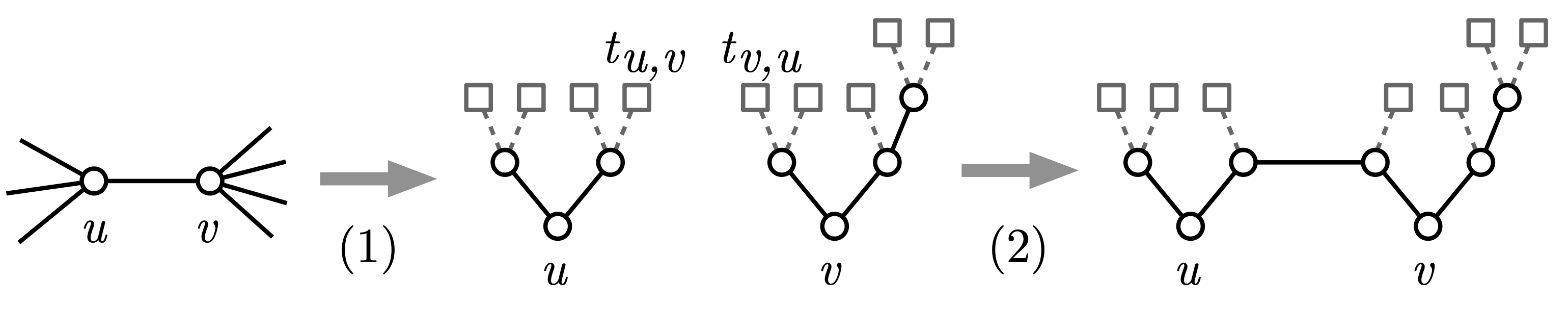
We now present the approximation algorithm itself. The algorithm constructs the host graph in two simple steps: first, for each node $v\in V$ separately, we construct a Huffman tree for the distribution $p_{v}$ , i.e., the conditional distribution of the other endpoint given that $v$ is included in the demand edge. Second, we connect these trees together to obtain the final host graph.

In more detail, the algorithm constructs the host graph $G$ as follows:

1.

For each node $v\in V$ , let $T_{v}$ be the $(\Delta-1)$ -ary Huffman tree for probability distribution $p_{v}$ , ignoring any probabilities of $0$ . Denote the leaf node corresponding to probability $p_{v}(u)$ as $t_{v,u}$ , and let $d_{T_{v}}(v,t_{v,u})$ be the distance from $v$ to $t_{v,u}$ in $T_{v}$ .

In the special case that $p_{v}(u)=1$ for some $u\in V$ , we take $T_{v}$ to be a tree with a root and a single leaf instead of the trivial tree.
2.

For each pair $\{u,v\}\subseteq V$ with $p(\{u,v\})\neq 0$ , we add an edge between the parent of $t_{v,u}$ in $T_{v}$ and the parent of $t_{u,v}$ in $T_{u}$ , and remove the nodes $t_{v,u}$ and $t_{u,v}$ .

See Figure 1 for illustration.

Refer to caption — Figure 1: Approximation algorithm for bounded network design with Steiner nodes. In Step (1), a Huffman tree is constructed for all nodes; the leaf nodes marked by squares are not included in the final host graph. In Step (2), the corresponding leaf nodes are deleted and replaced by an edge.

Time complexity.

To analyze the time complexity of the approximation algorithm, we first observe that constructing the Huffman tree in Step (1) for node $v$ takes $\mathcal{O}(d_{v}\log d_{v})$ time, where $d_{v}=\deg_{D}(v)$ is the degree of $v$ in the demand graph. We have

\sum_{v\in V}d_{v}\log_{2}d_{v}\leq\log_{2}m\sum_{v\in V}d_{v}=2m\log_{2}m\,,

and thus constructing Huffman trees for all nodes takes $\mathcal{O}(m\log n)$ time in total. Step (2) can clearly also be implemented in $\mathcal{O}(m\log n)$ time, so the total time complexity is $\mathcal{O}(m\log n)$ .

Cost of solution.

Consider a graph $G$ as constructed above. By construction, we have

d_{G}(u,v)=d_{T_{v}}(v,t_{v,u})+d_{T_{u}}(u,t_{u,v})-1

for all $u,v\in V$ . Thus, the expected path length between nodes in $V$ in $G$ is

		$\displaystyle\sum_{\{u,v\}\in\binom{V}{2}}p(\{u,v\})\bigl{(}d_{T_{v}}(v,t_{v,u% })+d_{T_{u}}(u,t_{u,v})-1\bigr{)}$
	$\displaystyle=\$	$\displaystyle\sum_{v\in V}\sum_{u\in V\setminus\{v\}}p(\{u,v\})d_{T_{v}}(v,t_{% v,u})-\sum_{\{u,v\}\in\binom{V}{2}}p(\{u,v\})$
	$\displaystyle=\$	$\displaystyle\sum_{v\in V}p(v)\sum_{u\in V}p_{v}(u)d_{T_{v}}(v,t_{v,u})-1$
	$\displaystyle\leq\$	$\displaystyle\sum_{v\in V}p(v)\Bigl{(}H_{\Delta-1}(p_{v})+1\Bigr{)}-1$
	$\displaystyle=\$	$\displaystyle\sum_{v\in V}p(v)H_{\Delta-1}(p_{v})+\sum_{v\in V}p(v)-1$
	$\displaystyle=\$	$\displaystyle\sum_{v\in V}p(v)H_{\Delta-1}(p_{v})+1\,\,\,\,:=C\$

The expected path length $C^{*}$ of an optimal solution is $\frac{1}{2}\sum_{v\in V}p(v)H_{\Delta+1}(p_{v})-1$ or greater by Theorem 3. Comparing this to the expected path length upper bound $C$ on $G$ , we have that the approximation factor of the algorithm is $\frac{2\log_{2}(\Delta+1)}{\log_{2}(\Delta-1)}+o(1)$ . Note that $\frac{2\log_{2}(\Delta+1)}{\log_{2}(\Delta-1)}$ is at most $4$ for all $\Delta\geq 3$ , and at most $3$ for all $\Delta\geq 4$ .

Number of nodes.

Let $n=|V|$ and let $m$ be the number of non-zero entries in $p$ . We now want to analyze the total number of nodes in $V\cup U$ in the graph $G$ given by the above algorithm.

Fact 7 (e.g. [27]).

Given a $d$ -ary Huffman tree $T$ , the leaves can be rearranged so that all internal nodes of $T$ have exactly $d$ children, with the exception of one internal node located at the maximum distance from the root. This node has at least $2$ children.

Fact 8.

A full $d$ -ary tree with $\ell$ leaves has $\frac{\ell-1}{d-1}$ internal nodes.

Now consider the Huffman tree $T_{v}$ constructed in Step (1) of the algorithm. Let $d=\Delta-1$ be the arity of the Huffman trees. Denoting the outdegree of $v$ in $p$ by $\deg(v)$ , and assuming $\deg(v)\geq 2$ , we have that $T_{v}$ has $\deg(v)$ leaves. By Fact 7, we can turn $T_{v}$ into a full $d$ -ary tree by adding at most $d-2$ leaves, which has $\ell\leq\deg(v)+d-2$ leaves. By Fact 8 it has at most

\frac{\ell-1}{d-1}\leq\frac{\deg(v)-1+d-2}{d-1}=\frac{\deg(v)-2}{d-1}+1

internal nodes; this is also an upper bound for the number of internal nodes in $T_{v}$ .

In the special case $\deg(v)=1$ , the above bound does not hold. However, we can use a slightly looser bound of $\frac{\deg(v)-1}{d-1}+1$ to cover all cases.

Since the leaf nodes of the Huffman trees $T_{v}$ are deleted in Step 2 of the algorithm, the total number of nodes in $G$ is the total number of internal nodes in these trees – note that the roots of the trees $T_{v}$ correspond to the original nodes in $V$ . Thus, the number of nodes in $G$ is at most

\displaystyle\sum_{v\in V}\Bigl{(}\frac{\deg(v)-1}{d-1}+1\Bigr{)}=\Bigl{(}1-% \frac{1}{d-1}\Bigr{)}n+\sum_{v\in V}\frac{\deg(v)}{d-1}\leq\Bigl{(}1-\frac{1}{% d-1}\Bigr{)}n+\frac{2}{d-1}m

(3)

5 Applications

This section discusses applications of our approach. First, we will use it to derive improved approximation bounds for the original demand-aware network design problem which results in a constant-factor approximation for the case where the maximum degree is close the average degree of the demand graph. Second, we show how it can be used to obtain efficient heuristics.

5.1 Improved approximation algorithm for demand balancing

In this section, we use the ideas from our approximation algorithm for bounded network design with Steiner nodes to design a demand balancing algorithm in the spirit of the results of Avin et al. [8]. That is, we consider a demand graph with average degree $\Delta_{\text{avg}}{}$ , but with possibly some nodes with very high degree, and we want to design a host graph without Steiner nodes that has maximum degree close to $\Delta_{\text{avg}}{}$ .

Here, we give an improved version of Theorem 4 of [8], showing how to construct a host graph with maximum degree $4\Delta_{\text{avg}}{}+1$ and better expected path length guarantees. Specifically, we improve the maximum degree guarantee from $12\Delta_{\text{avg}}{}$ to $4\Delta_{\text{avg}}{}+1$ and the expected path length guarantee by a factor of $\log_{2}(2\Delta_{\text{avg}}{})$ , which results in a constant-factor approximation.

5.1.1 Algorithm

For technical convenience, we assume $\Delta_{\text{avg}}{}$ is an integer and $n$ is divisible by $2$ . We say that a node $v$ is a high-degree node if its degree $\deg(v)$ in the demand graph satisfies $\deg(v)>2\Delta_{\text{avg}}{}$ , and otherwise we say it is a low-degree node. By Markov’s inequality, the number of high-degree nodes is at most $n/2$ .

For each node $v$ , we say that the up to $2\Delta_{\text{avg}}{}$ demand graph edges $\{u,v\}$ for which $p_{v}(u)$ are highest are the high-demand edges for $v$ , and the rest of the edges are low-demand edges for $v$ . Note that only heavy nodes have low-demand edges.

We now construct the host graph $G=(V,E)$ in two steps as follows.

Step 1: Low-demand trees.

For a heavy node $v$ , let $L_{v}$ and $H_{v}$ be the set of neighbours $u$ of $v$ in the demand graph such that $\{u,v\}$ is low-demand and high-demand, respectively. Define a distribution $q_{v}$ on $L_{v}$ by selecting an arbitrary node $s\in L_{v}$ and setting

q_{v}(u)=\begin{cases}p_{v}(u)+\sum_{w\in H_{v}}p_{v}(w)&\text{if $u=s$, and}% \\ p_{v}(u)&\text{otherwise.}\end{cases}

As in Section 4, we construct a $2\Delta_{\text{avg}}{}$ -ary Huffman tree for terminal set $L_{v}$ wrt. the probabilities $q_{v}(u)$ . As before, denote the leaf node corresponding to probability $u$ as $t_{v,u}$ , and let $d_{T_{v}}(v,t_{v,u})$ be the distance from $v$ to $t_{v,u}$ in $T_{v}$ .

We repeat the construction for all heavy nodes, and map the internal nodes of the trees injectively to nodes of $V$ so that root of the tree for $v$ is $v$ . We then add all edges of the tree to the routing graph $G$ . This is always possible, since by applying (3) with $N=n/2$ , $M=\Delta_{\text{avg}}{}n/2$ , and $d=2\Delta_{\text{avg}}{}$ , we have that there are at most $n$ internal nodes, including the roots, in the constructed trees.

Step 2: Connecting edges.

Now consider edge $\{u,v\}$ in the demand graph. There are three cases to consider:

1.

Edge $\{u,v\}$ is high-demand for both $u$ and $v$ . In this case, we add edge $\{u,v\}$ to $G$ .
2.

Edge $\{u,v\}$ is low-demand for both $u$ and $v$ . In this case, we add an edge from the parent node of $t_{v,u}$ to the parent node of $t_{u,v}$ to $G$ .
3.

Otherwise, without loss of generality, edge $\{u,v\}$ is high-demand for $u$ and low-demand for $v$ . In this case, we add an edge from $u$ to the parent of $t_{v,u}$ to $G$ .

5.1.2 Analysis

Time complexity.

By the same argument as in Section 4, we can see that computing the high-demand edges and building the Huffman trees for low-demand edges can be done in time $\mathcal{O}(m\log n)$ in total. All other steps of the algorithm can be implemented with at most $\mathcal{O}(m\log n)$ time.

Maximum degree.

Low-demand trees constructed in Step 1 have arity $2\Delta_{\text{avg}}{}$ , and thus contribute at most $2\Delta_{\text{avg}}{}+1$ to the degree of each node. This includes edges added for low-demand edges. Moreover, each node has at most $2\Delta_{\text{avg}}{}$ edges added for handling high-demand edges, for a total of $4\Delta_{\text{avg}}{}+1$ .

Expected path length.

Here we show that the expected path length in $G$ is at most $\sum_{u\in V}p(u)H_{2\Delta_{\text{avg}}{}}(p_{u})+1$ . First, let us recall the grouping rule for entropy.

Lemma 9.

Let $p\colon\{1,2,\dotsc,m\}$ be a distribution, and let $q\colon\{1,2,\dotsc,m-1\}$ be a distribution defined by $q(i)=p(i)$ for $i=1,2,\dotsc,m-1$ , and $q(m-1)=p(m-1)+p(m)$ . Then

H_{d}(p)=H_{d}(q)+(p(m-1)+p(m))H_{d}\Bigl{(}\frac{p(m-1)}{p(m-1)+p(m)},\frac{p% (m)}{p(m-1)+p(m)}\Bigr{)}

It follows immediately from Lemma 9 that for a heavy node $v$ we have $H_{d}(q_{v})\leq H_{d}(p_{v})$ for any $d\geq 2$ .

Now consider a non-zero demand $\{u,v\}$ . There are four cases to consider for the distance between $u$ and $v$ in $G$ :

1.

$u\in H_{v},v\in H_{u}$ : distance is $d_{G}(u,v)=1$ .
2.

$u\in H_{v},v\in L_{u}$ : distance is $d_{G}(u,v)=d_{T_{u}}(u,t_{u,v})$ .
3.

$u\in L_{v},v\in H_{u}$ : distance is $d_{G}(u,v)=d_{T_{v}}(v,t_{v,u})$ .
4.

$u\in L_{v},v\in L_{u}$ : distance is $d_{G}(u,v)=d_{T_{v}}(v,t_{v,u})+d_{T_{u}}(u,t_{u,v})-1$ .

Let $D$ be the set of demand edges, i.e., edges with non-zero demand. For a predicate $P$ , denote by $[P]$ a function that is $[P]=1$ if predicate $P$ is true, and $[P]=0$ otherwise. The expected path length in $G$ is now

\!\!\!\!\!\!\!\!\!\!\sum_{\{u,v\}\in D}\!\!\!\!p(\{u,v\})\Bigl{(}[u\in H_{v}][% v\in H_{u}]+[u\in H_{v}][v\in L_{u}]d_{T_{u}}(u,t_{u,v})+[u\in L_{v}][v\in H_{% u}]d_{T_{v}}(v,t_{v,u})\\ +[u\in L_{v}][v\in L_{u}](d_{T_{v}}(v,t_{v,u})+d_{T_{u}}(u,t_{u,v})-1)\Bigr{)}\,.

By re-grouping terms, this is equal to

	$\displaystyle\sum_{\{u,v\}\in D}p(\{u,v\})\Bigl{(}d_{T_{v}}(v,t_{v,u})\bigl{(}% [u\in H_{v}][v\in L_{u}]+[u\in L_{v}][v\in H_{u}]\bigr{)}$
	$\displaystyle+d_{T_{u}}(u,t_{u,v})\bigl{(}[u\in H_{v}][v\in L_{u}]+[u\in L_{v}% ][v\in L_{u}]\bigr{)}$
	$\displaystyle+[u\in H_{v}][v\in H_{u}]-[u\in L_{v}][v\in L_{u}]\Bigr{)}\,.$

By omitting the last negative term, and rearranging further, this is at most

		$\displaystyle\sum_{u\in V}\sum_{v\in L_{u}\cup H_{u}}p(\{u,v\})\Bigl{(}d_{T_{u% }}(u,t_{u,v})\bigl{(}[u\in H_{v}][v\in L_{u}]$
		$\displaystyle+[u\in L_{v}][v\in L_{u}]\bigr{)}+[u\in H_{v}][v\in H_{u}]\Bigr{)}$
	$\displaystyle\leq$	$\displaystyle\sum_{u\in V}\Bigl{(}\sum_{v\in L_{u}}p(\{u,v\})d_{T_{u}}(u,t_{u,% v})+\sum_{v\in H_{u}}p(\{u,v\})\Bigr{)}$
	$\displaystyle\leq$	$\displaystyle\sum_{u\in V}p(u)\Bigl{(}\sum_{v\in L_{u}}p_{u}(v)d_{T_{u}}(u,t_{% u,v})+\sum_{v\in H_{u}}p_{u}(v)\Bigr{)}\,.$

For fixed $u\in V$ , we have

	$\displaystyle\sum_{v\in L_{u}}p_{u}(v)d_{T_{u}}(u,t_{u,v})+\sum_{v\in H_{u}}p_% {u}(v)$
	$\displaystyle\leq\sum_{v\in L_{u}}p_{u}(v)d_{T_{u}}(u,t_{u,v})+\sum_{v\in H_{u% }}p_{u}(v)d_{T_{u}}(u,t_{u,s})$
	$\displaystyle=\sum_{v\in L_{u}\setminus\{s\}}p_{u}(v)d_{T_{u}}(u,t_{u,v})+% \Bigl{(}p_{u}(s)+\sum_{v\in H_{u}}p_{u}(v)\Bigr{)}d_{T_{u}}(u,t_{u,s})$
	$\displaystyle=\sum_{v\in L_{u}}q_{u}(v)d_{T_{u}}(u,t_{u,v})$
	$\displaystyle\leq H_{2\Delta_{\text{avg}}{}}(q_{u})+1\leq H_{2\Delta_{\text{% avg}}{}}(p_{u})+1\,.$

Thus, the expected path length in $G$ is at most

\sum_{u\in V}p(u)H_{2\Delta_{\text{avg}}{}}(p_{u})+1\,.

In comparison, by Theorem 3 the expected path length for degree- $(4\Delta_{\text{avg}}{}+1)$ host graphs is at least $\frac{1}{2}\sum_{u\in V}p(u)H_{4\Delta_{\text{avg}}{}+2}(p_{u})$ , meaning that $G$ is a constant-factor approximation for the optimal degree- $(4\Delta_{\text{avg}}+1)$ host graph.

5.2 Fixed-degree heuristics

The main challenge of our methods, as well as the prior work, is that we do not have approximation algorithms for bounded network designs that strictly respect a given arbitrary degree bound, without using additional resources such as Steiner nodes. However, in practice we expect that parameters such as the degree bound and number of Steiner nodes are limited by the physical properties of the network infrastructure, so solutions respecting these limitations would be required.

We describe a few heuristics which although do not have any guarantees on the quality of their solution, nevertheless appeared to have worked well in our experiments.

Fixed-degree heuristic.

We choose a subset of edges from the demand graph with large weights and use the Steiner node insertion algorithm to construct a DAN with maximum degree $\Delta-3$ for these edges. The number of picked edges is low enough to guarantee that we only need at most $n$ nodes for the construction of the DAN. Lastly, a randomly chosen (almost) $3$ -regular graph is overlaid on top of this DAN.

Random tree and random graph.

We simply pick a randomly chosen $\Delta-1$ -ary tree or (nearly) $\Delta$ regular graph as the demand aware graph. This is oblivious to the actual demand, but tends to have low diameter.

Greedy edge deletion.

We initially use the demand graph as the DAN. We iteratively delete edges of low weight incident on vertices with degree greater than the degree bound $\Delta$ . Deleting an edge may disconnect the graph and result in infinite expected path length. We do not delete edges if it would disconnect the graph, but as a result we may violate the degree bound $\Delta$ , in which case we say the algorithm failed.

Greedy edge selection.

We start with an empty DAN and iteratively add edges from the demand graph starting with the ones with highest weight. We do not add an edge if it would exceed the degree bound $\Delta$ . The algorithm may fail to construct a connected graph.

6 Empirical Evaluation

In this section we complement our theoretical insights with empirical evaluations using datacenter traces.

6.1 Methodology

All presented algorithms in this paper were implemented and evaluated in simulations. Furthermore, we provide comparisons to other methods such as the algorithm for sparse distributions from Theorem 4 by Avin et al. [8], which we will refer to as the Helper algorithm, and a $k$ -root graph approach by Peres and Avin [34], where $k=\log\Delta(D)$ , where $\Delta(D)$ is the maximum degree in the demand graph, which we will refer to as the Split&Join algorithm. For a full overview of the algorithms used in the experiments see Table 1.

Unfortunately, obtaining optimal solutions for our problem using integer linear programming was not feasible. We need $\mathcal{O}(n^{2})$ binary variables representing each possible edge in the output graph and for modeling the expected path length in the resulting graph we needed a cubic number of integer variables. Solving these ILPs was feasible for only very small instances.

Table 1: Overview of the algorithms used in the experiments. The Steiner nodes column refers to whether an algorithm solves the bounded network design problem with or without Steiner nodes.

Name	Shorthand	Ref.	Steiner nodes	$\Delta$ as input
Steiner Node Insertion	SNI	Section 4	yes	yes
Demand Balancing	DB	Section 5.1	no	no
Split&Join	S&J	Split&Join [34]	no	no
Helper	Help	Theorem 4 in [8]	no	no
Fixed-degree	Fix-Deg	Section 5.2	no	yes
Random Tree	Rnd-Tree	Section 5.2	no	yes
Random Graph	Rnd-Graph	Section 5.2	no	yes
Greedy Edge Deletion	GED	Section 5.2	no	yes
Greedy Edge Selection	GES	Section 5.2	no	yes

Dataset.

For the experiments we used the real-world datacenter trace collection from Avin et al. [5] that was also used by previous works [10, 34, 8]. These traces contain temporal data, specifically source, destination and timestamps of communicating nodes. To adapt these traces to our demand graph input format, we create an edge between two communicating nodes and set its weight equal to number of times the nodes communicated. The weights are normalized so that this can be interpreted as a communication distribution (demand). In Appendix B in Table 4 some selected parameters of these instances are summarized.

6.2 Results

We divide the results of the experiments into three groups, based on the algorithms which they involve, similar to the grouping in Table 1.

Sparse heuristics.

We first focus our attention on the bounded network design heuristics for which the maximum degree is a function of the input demand graph and cannot be specified by the user. In Table 2 properties of the resulting host graphs computed by these algorithms on our network trace dataset are presented. The Helper heuristic appeared to have the highest expected path length and second largest maximum degree compared to the other three approaches. In contrast, the Demand Balancing heuristic achieved the lowest expected path length while also having the lowest maximum degree, except for three demand graphs. For four of the ten demand graphs the expected path lengths for the Demand Balancing and Split&Join heuristics were almost a third of the expected path length of the Helper heuristic. The Split&Join heuristic achieved a low expected path length, but at the cost of having a comparatively large maximum degree, almost double that of the Demand Balancing heuristic for three demand graphs.

Table 2: Properties of the host graphs computed by the Split&Join, Helper, Demand Balancing (DB) heuristics. We denote by

\Delta

the maximum degree in the host graph and by EPL its expected path length. For each trace we highlight in gray the lowest maximum degree and in yellow the lowest expected path length, unless there is a tie.

	Split&Join		Helper		DB
Trace	$\Delta$	EPL	$\Delta$	EPL	$\Delta$	EPL
fb-cluster-rack-A	$507$	$1.33$	$399$	$3.26$	290	1.31
fb-cluster-rack-B	$1{,}305$	$1.06$	$855$	$4.25$	754	1.05
fb-cluster-rack-C	$1{,}460$	$1.14$	$870$	$3.51$	683	1.08
hpc-cesar-mocfe	$21$	$1.33$	18	$2.87$	$21$	1.0
hpc-cesar-nekbone	$39$	$1.07$	$36$	$1$	$36$	$1$
hpc-boxlib-cns	$157$	$1.11$	102	$1.04$	$293$	1.01
hpc-boxlib-multigrid	$31$	$1.12$	$26$	$1$	$26$	$1$
p-fabric-trace-0-1	143	$1.01$	$144$	$1$	$144$	$1$
p-fabric-trace-0-5	$143$	$1.01$	$143$	$1$	$143$	$1$
p-fabric-trace-0-8	$143$	$1.01$	$143$	$1$	$143$	$1$

Fixed degree heuristics.

We next compare different heuristics for which the maximum degree is an input parameter. In Figure 2 the average expected path length over our whole dataset is plotted against the maximum degree constraint for different heuristics. It is apparent that the two heuristics that are oblivious to the demand graph, namely the Random Tree and Random Graph heuristics have the worst expected path length, which was expected to due their obliviousness to the input.

Figure 2: Average expected path length over the whole datacenter trace dataset depending on the maximum desired degree

\Delta

. The results for the Random Tree, Random Graph, Fixed-degree, and Steiner Node Insertion heuristics are depicted. The results are averaged over 10 different runs. Heuristics which sometimes failed are not depicted.

Unsurprisingly, the Random Tree heuristic is significantly worse than for example the Random Graph heuristic. The randomly constructed $(\Delta-1)$ -ary tree has many leaves which by definition have a degree of one, and are thus poorly utilized as more edges could be inserted to improve the EPL.

In Table 3 we present results from Figure 2 for the case $\Delta=32$ in more detail, and also include some results for heuristics which failed do solve some instances. For the Facebook instances the Fixed-degree heuristic has the lowest expected path length. For some demands the heuristics achieve an expected path length of almost one, whereas the Random Graph and Tree heuristics have at least double the expected path length. The Greedy Edge Deletion and Greedy Edge Selection fail on the Facebook instances.

Table 3: Summary of the expected path length of the host graphs computed by the Fixed-degree, Random Tree, Random Graph, Greedy Edge Deletion, and Greedy Edge Selection heuristics for

\Delta=32

. If an algorithm failed on some instance then it is replaced with a “—” symbol. For each trace we highlight in gray the lowest expected path length, unless there is a tie.

Trace	Fix-Deg	Rnd Graph	Rnd Tree	GED	GES
fb-cluster-rack-A	2.6	$3.02$	$5.72$	–	–
fb-cluster-rack-B	2.48	$3.13$	$5.78$	–	–
fb-cluster-rack-C	2.69	$3.28$	$5.86$	–	–
hpc-cesar-mocfe	$1$	$2.32$	$3.87$	$1$	$1$
hpc-cesar-nekbone	$1.01$	$2.32$	$3.87$	$1$	$1$
hpc-boxlib-cns	$2.2$	$2.33$	$3.87$	$1.88$	1.85
hpc-boxlib-multigrid	$1$	$2.32$	$3.87$	$1$	$1$
p-fabric-trace-0-1	$1.37$	$1.78$	$3.22$	$1.29$	–
p-fabric-trace-0-5	$1.41$	$1.77$	$3.21$	$1.28$	1.27

Steiner nodes.

Our last experiments involve the Steiner Node Insertion algorithm. Recall, that the Steiner Node Insertion algorithm is allowed to use additional nodes (Steiner nodes) that are not present in the demand graph. For a relatively low maximum degree of eight the number of new nodes used by the algorithm is sometimes even greater than $30n$ . As the maximum degree increases, the expected path length decreases and so does the number of used Steiner nodes. For some traces the number of Steiner nodes remains quite high. For example, for $\Delta=64$ on the second Facebook trace the algorithm used $2.7n$ Steiner nodes.

Furthermore, in Figure 2 we compare the Steiner Node Insertion algorithm to the Fixed-degree heuristic which utilizes the Steiner Node Insertion algorithm, but does not use Steiner nodes; that is, it computes a host graph with the same vertex set as the demand graph. It can be observed that the Steiner Node Insertion algorithm achieves a slightly lower expected path length on average, but as can be seen in Table 5 (Appendix B) this is at the cost of utilizing many Steiner nodes. The Fixed-degree does not utilize Steiner nodes, but the expected path length is marginally larger.

7 Conclusion

This paper presented new approaches to designing bounded-degree demand-aware networks, leading to improved approximation algorithms as well as heuristics for variants of the problem. We also presented various hardness results and lower bounds. From the extensive empirical evaluation, we highlight our fixed-degree heuristic as a practical algorithm for bounded-degree network design problem; it is guaranteed to respect the given degree bound regardless of the demand distribution and, in experiments, achieves expected paths lengths close to optimal on real-world instances.

Our work leaves open several interesting directions for future research. In particular, it will be interesting to explore the tradeoff between approximation quality and resource augmentation. More generally, it remains open whether a constant-factor approximation algorithm exists for bounded-degree network design without augmentation.

References

[1] Vamsi Addanki, Chen Avin, and Stefan Schmid. Mars: Near-optimal throughput with shallow buffers in reconfigurable datacenter networks. Proc. ACM Meas. Anal. Comput. Syst., 7(1), March 2023. doi:10.1145/3579312.
[2] Daniel Amir, Nitika Saran, Tegan Wilson, Robert Kleinberg, Vishal Shrivastav, and Hakim Weatherspoon. Shale: A practical, scalable oblivious reconfigurable network. In Proceedings of the ACM SIGCOMM 2024 Conference, ACM SIGCOMM ’24, pages 449–464, New York, NY, USA, 2024. Association for Computing Machinery. doi:10.1145/3651890.3672248.
[3] Daniel Amir, Tegan Wilson, Vishal Shrivastav, Hakim Weatherspoon, Robert Kleinberg, and Rachit Agarwal. Optimal oblivious reconfigurable networks. In Proceedings of the 54th Annual ACM SIGACT Symposium on Theory of Computing, STOC 2022, 2022. doi:10.1145/3519935.3520020.
[4] Chen Avin, Manya Ghobadi, Chen Griner, and Stefan Schmid. On the complexity of traffic traces and implications. In Proc. ACM SIGMETRICS, 2020.
[5] Chen Avin, Manya Ghobadi, Chen Griner, and Stefan Schmid. On the complexity of traffic traces and implications. Proceedings of the ACM on Measurement and Analysis of Computing Systems, 4(1):1–29, 2020. doi:10.1145/3379486.
[6] Chen Avin, Alexandr Hercules, Andreas Loukas, and Stefan Schmid. rDAN: Toward robust demand-aware network designs. Information Processing Letters, 133:5–9, 2018. doi:10.1016/J.IPL.2017.12.008.
[7] Chen Avin, Kaushik Mondal, and Stefan Schmid. Demand-aware network designs of bounded degree. In Proc. International Symposium on Distributed Computing (DISC), 2017.
[8] Chen Avin, Kaushik Mondal, and Stefan Schmid. Demand-aware network designs of bounded degree. Distributed Computing, 33(3):311–325, 2020. doi:10.1007/S00446-019-00351-5.
[9] Chen Avin, Kaushik Mondal, and Stefan Schmid. Demand-aware network design with minimal congestion and route lengths. IEEE/ACM Transactions on Networking, 30(4):1838–1848, 2022. doi:10.1109/TNET.2022.3153586.
[10] Chen Avin and Stefan Schmid. Renets: Statically-optimal demand-aware networks. In Symposium on Algorithmic Principles of Computer Systems (APOCS), pages 25–39. SIAM, 2021. doi:10.1137/1.9781611976489.3.
[11] Chen Avin and Stefan Schmid. Renets: Statically-optimal demand-aware networks. In Proc. SIAM Symposium on Algorithmic Principles of Computer Systems (APOCS), 2021.
[12] Hitesh Ballani, Paolo Costa, Raphael Behrendt, Daniel Cletheroe, Istvan Haller, Krzysztof Jozwik, Fotini Karinou, Sophie Lange, Kai Shi, Benn Thomsen, et al. Sirius: A flat datacenter network with nanosecond optical switching. In Proceedings of the Annual conference of the ACM Special Interest Group on Data Communication on the applications, technologies, architectures, and protocols for computer communication, pages 782–797, 2020.
[13] Edward A Bender and E. Rodney Canfield. The asymptotic number of labeled graphs with given degree sequences. Journal of Combinatorial Theory, Series A, 24(3):296–307, 1978. doi:10.1016/0097-3165(78)90059-6.
[14] NM Mosharaf Kabir Chowdhury, Muntasir Raihan Rahman, and Raouf Boutaba. Virtual network embedding with coordinated node and link mapping. In IEEE INFOCOM 2009, pages 783–791. IEEE, 2009.
[15] Thomas M. Cover and Joy A. Thomas. Elements of information theory. Wiley-Interscience, 2006.
[16] Fred Douglis, Seth Robertson, Eric Van den Berg, Josephine Micallef, Marc Pucci, Alex Aiken, Maarten Hattink, Mingoo Seok, and Keren Bergman. Fleet—fast lanes for expedited execution at 10 terabits: Program overview. IEEE Internet Computing, 25(3):79–87, 2021. doi:10.1109/MIC.2021.3075326.
[17] Nathan Farrington and Alexey Andreyev. Facebook’s data center network architecture. In 2013 Optical Interconnects Conference, pages 49–50. IEEE, 2013.
[18] Aleksander Figiel, Leon Kellerhals, Rolf Niedermeier, Matthias Rost, Stefan Schmid, and Philipp Zschoche. Optimal virtual network embeddings for tree topologies. In Proceedings of the 33rd ACM Symposium on Parallelism in Algorithms and Architectures, pages 221–231, 2021. doi:10.1145/3409964.3461787.
[19] Aleksander Figiel, Darya Melnyk, Andre Nichterlein, Arash Pourdamghani, and Stefan Schmid. Spiderdan: Matching augmentation in demand-aware networks. In SIAM Symposium on Algorithm Engineering and Experiments (ALENEX), 2025.
[20] M. R. Garey, D. S. Johnson, and L. Stockmeyer. Some simplified NP-complete graph problems. Theoretical Computer Science, 1(3):237–267, 1976. doi:10.1016/0304-3975(76)90059-1.
[21] Michael R. Garey and David S. Johnson. Computers and Intractability. W.H. Freeman and Company, 1979.
[22] Monia Ghobadi, Ratul Mahajan, Amar Phanishayee, Nikhil Devanur, Janardhan Kulkarni, Gireeja Ranade, Pierre-Alexandre Blanche, Houman Rastegarfar, Madeleine Glick, and Daniel Kilper. Projector: Agile reconfigurable data center interconnect. In Proceedings of the 2016 ACM SIGCOMM Conference, pages 216–229. ACM, 2016. doi:10.1145/2934872.2934911.
[23] Chen Griner, Johannes Zerwas, Andreas Blenk, Manya Ghobadi, Stefan Schmid, and Chen Avin. Cerberus: The power of choices in datacenter topology design (a throughput perspective). Proc. ACM Meas. Anal. Comput. Syst., 5(3), December 2021. doi:10.1145/3491050.
[24] Matthew Nance Hall, Klaus-Tycho Foerster, Stefan Schmid, and Ramakrishnan Durairajan. A survey of reconfigurable optical networks. Optical Switching and Networking, 41:100621, 2021. doi:10.1016/J.OSN.2021.100621.
[25] Navid Hamedazimi, Zafar Qazi, Himanshu Gupta, Vyas Sekar, Samir R. Das, Jon P. Longtin, Himanshu Shah, and Ashish Tanwer. Firefly: a reconfigurable wireless data center fabric using free-space optics. SIGCOMM Comput. Commun. Rev., 44(4):319–330, August 2014. doi:10.1145/2740070.2626328.
[26] Monika Henzinger, Stefan Neumann, and Stefan Schmid. Efficient distributed workload (re-) embedding. Proc. ACM SIGMETRICS, 2019.
[27] Stefan Höst. Information and Communication Theory. Wiley-IEEE Press, 2019.
[28] Wolfgang Kellerer, Patrick Kalmbach, Andreas Blenk, Arsany Basta, Martin Reisslein, and Stefan Schmid. Adaptable and data-driven softwarized networks: Review, opportunities, and challenges. Proceedings of the IEEE, 107(4):711–731, 2019. doi:10.1109/JPROC.2019.2895553.
[29] Vincenzo Liberatore. Circular arrangements. In Proc. International Colloquium on Automata, Languages, and Programming (ICALP 2002), pages 1054–1065. Springer, 2002. doi:10.1007/3-540-45465-9_90.
[30] Kurt Mehlhorn. Nearly optimal binary search trees. Acta Informatica, 5(4):287–295, 1975. doi:10.1007/BF00264563.
[31] William M Mellette, Rajdeep Das, Yibo Guo, Rob McGuinness, Alex C Snoeren, and George Porter. Expanding across time to deliver bandwidth efficiency and low latency. In Proc. 17th USENIX Symposium on Networked Systems Design and Implementation (NSDI 20), pages 1–18, 2020. URL: https://www.usenix.org/conference/nsdi20/presentation/mellette.
[32] William M Mellette, Rob McGuinness, Arjun Roy, Alex Forencich, George Papen, Alex C Snoeren, and George Porter. Rotornet: A scalable, low-complexity, optical datacenter network. In Proceedings of the Conference of the ACM Special Interest Group on Data Communication, pages 267–280. ACM, 2017. doi:10.1145/3098822.3098838.
[33] Alistair Moffat. Huffman coding. ACM Computing Surveys, 52(4), 2019. doi:10.1145/3342555.
[34] Or Peres and Chen Avin. Distributed demand-aware network design using bounded square root of graphs. In IEEE Conference on Computer communications (INFOCOM). IEEE, 2023. doi:10.1109/INFOCOM53939.2023.10228932.
[35] Arash Pourdamghani, Chen Avin, Robert Sama, Maryam Shiran, and Stefan Schmid. Hash & adjust: Competitive demand-aware consistent hashing. In International Conference on Principles of Distributed Systems (OPODIS), 2024. doi:10.4230/LIPIcs.OPODIS.2024.24.
[36] Leon Poutievski, Omid Mashayekhi, Joon Ong, Arjun Singh, Mukarram Tariq, Rui Wang, Jianan Zhang, Virginia Beauregard, Patrick Conner, Steve Gribble, et al. Jupiter evolving: transforming google’s datacenter network via optical circuit switches and software-defined networking. In Proc. ACM SIGCOMM 2022 Conference, pages 66–85, 2022.
[37] Matthias Rost and Stefan Schmid. Virtual network embedding approximations: Leveraging randomized rounding. IEEE/ACM Transactions on Networking, 27(5):2071–2084, 2019. doi:10.1109/TNET.2019.2939950.
[38] D.D. Sleator and R.E. Tarjan. Self-adjusting binary search trees. Journal of the ACM (JACM), 32(3):652–686, 1985. doi:10.1145/3828.3835.
[39] Min Yee Teh, Zhenguo Wu, and Keren Bergman. Flexspander: augmenting expander networks in high-performance systems with optical bandwidth steering. IEEE/OSA Journal of Optical Communications and Networking, 12(4):B44–B54, 2020. doi:10.1364/JOCN.379487.
[40] Tegan Wilson, Daniel Amir, Nitika Saran, Robert Kleinberg, Vishal Shrivastav, and Hakim Weatherspoon. Breaking the vlb barrier for oblivious reconfigurable networks. In Proceedings of the 56th Annual ACM Symposium on Theory of Computing, STOC 2024, 2024. doi:10.1145/3618260.3649608.
[41] Johannes Zerwas, C Gyorgyi, A Blenk, Stefan Schmid, and Chen Avin. Duo: A high-throughput reconfigurable datacenter network using local routing and control. In Proc. ACM SIGMETRICS, 2023.
[42] Mingyang Zhang, Jianan Zhang, Rui Wang, Ramesh Govindan, Jeffrey C Mogul, and Amin Vahdat. Gemini: Practical reconfigurable datacenter networks with topology and traffic engineering. CoRR, 2021. arXiv:2110.08374.

Appendix A Hardness of bounded-degree network design

Decision version of bounded-degree network design.

In this section, we show that the decision versions of bounded-degree network design, with or without Steiner nodes, is NP-complete for any fixed degree bound $\Delta\geq 2$ . Formally, the decision version bounded of bounded-degree network design is defined as follows – note that we consider an integer-weighted version of the problem to sidestep considerations regarding encoding of small fractional number:

Instance:

A set $V$ with $|V|=n$ , a weight function $w\colon\binom{V}{2}\to\mathbb{N}$ , positive integers $\Delta$ and $K$ .

Question:

Is the a graph $G=(V,E)$ such that maximum degree of $G$ is at most $\Delta$ and

\sum_{\{u,v\}\in\binom{V}{2}}w(\{u,v\})d_{G}(u,v)\leq K\,,

where $d_{G}(u,v)$ denotes the distance between $u$ and $v$ in $G$ .

The decision version of bounded-degree network design with Steiner nodes is defined analogously:

Instance:

A set $V$ with $|V|=n$ , a weight function $w\colon\binom{V}{2}\to\mathbb{N}$ , positive integers $\Delta$ and $K$ .

Question:

Is there a graph $G=(V^{\prime},E)$ such that $V\subseteq V^{\prime}$ , the maximum degree of $G$ is at most $\Delta$ , and

\sum_{\{u,v\}\in\binom{V}{2}}w(\{u,v\})d_{G}(u,v)\leq K\,,

where $d_{G}(u,v)$ denotes the distance between $u$ and $v$ in $G$ ?

While it is immediately clear that bounded-degree network design without Steiner nodes is in NP, it is not a priori clear that the version with Steiner nodes always has optimal host graphs of polynomial size. However, not surprisingly this is indeed the case:

Lemma 10.

For any instance of bounded-degree network design problem with Steiner nodes, there is a solution with optimal effective path length and at most a polynomial number of Steiner nodes.

Proof.

For $\Delta=2$ , one can immediately observe that there is a solution with optimal effective path length without Steiner nodes, as we can replace any degree- $2$ Steiner node with an edge. Thus, assume $\Delta\geq 3$ and let $G=(V\cup U,E)$ be a host graph with optimal effective path length for an instance of bounded-degree network design with Steiner nodes. Moreover, assume that $G$ is minimal in the sense that any proper subgraph of $G$ has larger effective path length.

Let $u,v\in V$ be arbitrary pair of nodes with non-zero demand between them and distance $\ell\geq 4$ in $G$ , and consider the shortest path $P=(u,v_{1},v_{2},\dotsc,v_{l-1},v)$ between $u$ and $v$ in $G$ . Let $s,t\in V$ be an another pair of nodes with non-zero demand between them, possibly including either $u$ or $v$ but not both. We say that an edge $e$ with exactly one endpoint on $P$ is critical for $s$ and $t$ if removing it from $G$ would increase the distance between $s$ and $t$ .

Consider a shortest path $P^{\prime}=(s=u_{0},u_{1},u_{2},\dotsc,u_{k-1},u_{k}=t)$ between $s$ and $t$ that intersects with $P$ , and let $u_{i}$ and $u_{j}$ be the first and the last node on $P^{\prime}$ that is also on $P$ , respectively. As both $P$ and $P^{\prime}$ are shortest paths, the distance between $u_{i}$ and $u_{j}$ must be the same along $P$ and $P^{\prime}$ . It follows that only $\{u_{i-1},u_{i}\}$ and $\{u_{j},u_{j+1}\}$ can be critical for $s$ and $t$ , if they exist. Moreover, a critical edge must be on all shortest paths between $s$ and $t$ , so there can be at most two critical edges for $s$ and $t$ .

Now consider an arbitrary edge $e\in E$ with exactly one endpoint on $P$ . By minimality of $G$ , deleting $e$ would increase the distance between some pair $\{s,t\}\subseteq V$ ; thus, edge $e$ is critical for some $s$ and $t$ . By choice of $e$ , it follows that all edges with exactly one endpoint on $G$ are critical for some $s$ and $t$ . By above argument, there are at most $2\binom{n}{2}\leq n^{2}$ critical edges, and thus at most that many edges with exactly one endpoint on $P$ .

Assume for the sake of contradiction that $\ell\geq n^{2}+3$ . Since there are at most $n^{2}$ edges with exactly one endpoint on $P$ , there exist two non-adjacent nodes on $P$ that have degree less than $\Delta$ . Adding an edge between these two nodes to $G$ would decrease the effective path length, which contradicts the optimality of $G$ . Moreover, since $u$ and $v$ were chosen arbitrarily, it holds that for all pairs $u,v\in V$ with non-zero demand the distance between $u$ and $v$ in $G$ is $O(n^{2})$ . By minimality of $G$ , it follows that $G$ has at most $O(n^{4})$ nodes. $\hfill\blacktriangleleft$

NP-completeness for $\Delta=2$ .

For degree bound $\Delta=2$ one can easily observe that, for both versions of the bounded-degree network problem, there is an optimal host graph that is a collection of cycles. Moreover, it is clear that Steiner nodes cannot improve the solution for $\Delta=2$ .

Avin et al. [8] have noted that for connected demand graphs, the bounded-degree network design problem for $\Delta=2$ is very close to minimum linear arrangement. More precisely, we can reduce from the undirected circular arrangement problem, known to be NP-complete [29], to prove that bounded-degree network design problems are NP-complete:

Instance:

Graph $G=(V,E)$ with $|V|=n$ , a weight function $w\colon E\to\mathbb{N}$ , a positive integer $K$ .

Question:

Is there a bijection $f\colon V\to\{1,2,\dotsc,n\}$ such that

\sum_{e\in E}w(e)h(e)\leq K\,,

where $h(\{u,v\})=\min\bigl{(}f(u)-f(v)\mod n,f(v)-f(u)\mod n)$ .

The circular arrangement problem can be seen as an instance of bounded-degree network design where the host graph is required to be a cycle. In particular, circular arrangement is equivalent to bounded-degree network design with $\Delta=2$ on connected instances, as in that case the host graph is also required to be connected – i.e., a path or a cycle. Thus, the NP-completeness for both versions of bounded-degree network design follows from the following observation:

Lemma 11.

Undirected circular arrangement problem is NP-complete when restricted to connected graphs.

Proof.

Membership in NP is trivial. For NP-hardness, we reduce from undirected circular arrangement on general inputs.

Let $G=(V,E)$ , $w$ and $K$ be an instance of undirected circular arrangement. We construct a new instance by letting $G^{\prime}=(V,E^{\prime})$ be a complete graph on $V$ , and define the new edge weight function $w^{\prime}$ as

w^{\prime}(e)=\begin{cases}n^{3}w(e)&\text{if $e\in E$, and }\\ 1&\text{if $e\notin E$.}\end{cases}

Finally, we set $K^{\prime}=n^{3}(K+1)-1$ . Clearly $G^{\prime}$ is a connected graph.

First consider the case where $G$ is a yes-instance, and let $f$ be a solution satisfying $\sum_{e\in E}w(e)h(e)\leq K$ . Using $f$ as a solution for $G^{\prime}$ and summing over the edges in $E$ , we have that $\sum_{e\in E}w^{\prime}(e)h(e)\leq n^{3}K$ . For edges not in $E$ , we have

\sum_{e\notin E}w^{\prime}(e)h(e)\leq\binom{n}{2}n<n^{3}\,.

Thus,

\sum_{e\in E^{\prime}}w^{\prime}(e)h(e)=\sum_{e\in E}w^{\prime}(e)h(e)+\sum_{e% \in E^{\prime}}w^{\prime}(e)h(e)<n^{3}K+n^{3}\,,

which is at most $n^{3}(K+1)-1$ as the value of the sum is an integer. Hence, $G^{\prime}$ is a yes-instance.

For the other direction, assume that $G^{\prime}$ a yes-instance, and let $f$ be a solution satisfying $\sum_{e\in E^{\prime}}w^{\prime}(e)h(e)\leq K^{\prime}$ . This implies that

\sum_{e\in E}w^{\prime}(e)h(e)\leq K^{\prime}=n^{3}(K+1)-1\,.

Since all edge weights $w^{\prime}(e)$ for $e\in E$ are divisible by $n^{3}$ , the value of $\sum_{e\in E}w^{\prime}(e)h(e)$ is also divisible by $n^{3}$ . This combined with above inequality implies

\sum_{e\in E}n^{3}w(e)h(e)\leq n^{3}K\,,

and thus we have

\sum_{e\in E}w(e)h(e)\leq K\,.

Hence, $G$ is a yes-instance. $\hfill\blacktriangleleft$

NP-completeness for $\Delta\geq 3$ .

We prove NP-hardness for both variants of the bounded-degree network design problem. There are two main tricks we utilize in this proof, which we explain before proceeding with the proof proper.

First is the observation that when we construct instances for these problems, we can force any optimal host graph to have some specific edge $\{u,v\}$ we desire by giving this pair a large demand $p(\{u,v\})=W$ . If we then have $k$ edges we want to force, we can set the cost threshold of the instance to be between $k W$ and $kW-1$ , so that any valid host graph will necessarily include all of these edges.

The second trick is used to ensure that nodes in our gadget constructions have the desired degrees. We use the following simple lemma:

Lemma 12.

Let $d\geq 3$ be an odd integer. There is a graph $H_{d}=(V,E)$ such that $|V|=d+2$ , one node in $H_{d}$ has degree $d-1$ , and all other nodes in $H_{d}$ have degree $d$ .

Proof.

We start from a $(d+1)$ -clique $K_{d+1}$ , and then remove an arbitrary matching of size $(d-1)/2$ . The resulting graph has $d-1$ nodes of degree $d-1$ , and 2 nodes of degree $d$ . We then add a new node and connect it with an edge to all the nodes of degree $d-1$ . The resulting graph clearly has the claimed properties. $\hfill\blacktriangleleft$

We use Lemma 12 to do what we will henceforth call attaching a degree-blocking gadget: given a graph of odd maximum degree $\Delta$ , some value $d\leq\Delta$ , and a node $v$ with degree $\deg(v)<d$ , we turn $v$ into a degree- $d$ node by adding $d-\deg(v)$ copies of $H_{\Delta}$ to the graph, and adding an edge between $v$ and degree- $(\Delta-1)$ node in each copy of $H_{\Delta}$ . Clearly then $v$ will have degree $d$ , and each added node will have degree exactly $\Delta$ .

We now proceed to the main proof. For simplicity, we start with the case of odd maximum degree $\Delta$ .

Theorem 13.

Bounded-degree network design and bounded-degree network design with Steiner nodes are NP-hard for any odd $\Delta\geq 3$ .

Proof.

We reduce from vertex cover on $3$ -regular graphs; recall that the problem is known to remain NP-complete even with the degree restriction [21, 20]. More precisely, we will give a reduction that has the additional property that the resulting instance is a yes-instance without Steiner nodes if and only if it is a yes-instance with Steiner nodes, thus proving NP-hardness for both variants of the problem.

Let $(V,E,k)$ be an instance of vertex cover (in its decision form, where we ask if there is a vertex cover of size $k$ ). We first define the various gadget graphs we will use in the the construction.

Selector gadget.

Let $b=2^{\lceil\log_{2}k\rceil}$ be the smallest power of two larger than $k$ . To construct the selector gadget, we start with a complete binary tree with $b$ leaves and root node $r$ . We arbitrarily select $k$ leaves as the selector nodes $s_{1},s_{2},\dotsc,s_{k}$ , and attach $\Delta-2$ degree-blocking gadgets $H_{\Delta}$ to each $s_{i}$ . We also attach $\Delta-2$ degree-blocking gadgets $H_{\Delta}$ to the root $r$ , and $\Delta-1$ degree-blocking gadgets to the remaining leaves. One can now verify that each selector node has degree $\Delta-1$ , and the remaining nodes in the selector gadget have degree $\Delta$ .

Vertex gadgets.

For each vertex $v\in V$ in the vertex cover instance, we construct a vertex gadget as follows – recall that by assumption $v$ has degree $3$ . We take a complete binary tree with $4$ leaves, denoting the root of the tree by $r_{v}$ . We identify $3$ of the leaves as terminal nodes $t_{e}$ for edges $e$ incident to node $v$ . Finally, we attach $\Delta-3$ degree-blocking gadgets $H_{\Delta}$ to the root $r_{v}$ , as well as $\Delta-2$ degree-blocking gadget to each terminal node and $\Delta-1$ degree-blocking gadgets to the remaining leaf.

Finally, we combine the vertex gadgets for all vertices in $V$ by identifying two terminal nodes for edge $e=\{u,v\}$ in the vertex gadgets of $u$ and $v$ , as well as merging the respective degree-blocking gadgets into one. We can now observe that in the graph formed by the combined vertex gadget, the root nodes $r_{v}$ for $v\in V$ have degree $\Delta-1$ , and all other nodes have degree $\Delta$ .

Instance construction.

We now construct an instance $(V^{\prime},w,K)$ of bounded-degree network design with Steiner nodes as follows. Let $V^{\prime}$ be the set of nodes in the selector gadget and the combined vertex gadgets as constructed above. For any edge $\{u,v\}\subseteq V^{\prime}$ in the gadget constructions, we set the demand $w(\{u,v\})$ to be $W=|E|(\log_{2}b+3)+1$ . For each edge $e\in E$ in the vertex cover instance, we add demand $w(\{r,t_{e}\})=1$ between the root of the selector gadget and the terminal node for $e$ . For all other pairs, we set the demand to $0$ . Finally, we set the effective path length threshold for the bounded network design instance to be $K=MW+|E|(\log_{2}b+3)$ , where $M$ is the total number of edges in the gadgets.

Correctness.

Now assume that $(V,E,k)$ is a yes-instance of vertex cover, and let $C=\{v_{1},v_{2},\dotsc,v_{k}\}\subseteq V$ be a vertex cover. Let $G^{\prime}=(V^{\prime},E^{\prime})$ be a host graph for instance $(V^{\prime},w,K)$ obtained by taking all the gadget edges and edges $\{s_{i},r_{v_{i}}\}$ for $i=1,2,\dotsc,k$ . The demands for the gadget edges are satisfied by $G^{\prime}$ with direct edges, contributing a total of $M W$ to the effective path length. Now consider an arbitrary edge $e\in E$ and a demand between $r$ and $t_{e}$ . Since $C$ is a vertex cover, there is a vertex $v_{i}\in C\cap e$ such that the edge $\{s_{i},r_{v_{i}}\}$ belongs to $E^{\prime}$ . Thus there is a path from $r$ to $t_{e}$ in $G^{\prime}$ that starts from $r$ and travels along the selector gadget to $s_{i}$ , crosses the edge $\{s_{i},r_{v_{i}}\}$ and travels from $r_{v_{i}}$ to $t_{e}$ along the vertex gadget for $v_{i}$ . This path has length $\log_{2}b+3$ . Since $e$ was selected arbitrarily and $C$ is a vertex cover, this holds for all edges $e\in E$ . Therefore the total effective path length is $MW+|E|(\log_{2}b+3)=K$ , that is, $(V^{\prime},w,K)$ is a yes-instance.

For the other direction, assume that $(V^{\prime},w,K)$ is a yes-instance, and let $G^{\prime}=(V^{\prime}\cup U,E^{\prime})$ be a host graph with effective path length at most $K$ . First, we observe that $G^{\prime}$ must include all gadget edges, as otherwise the effective path length from the corresponding demands is at least $(M+1)W>K$ . Now consider the path between $r$ and $t_{e}$ for an arbitrary $e\in E$ . Since all gadget edges are included in $G^{\prime}$ , this path must exit the selector gadget via an edge connected to one of the selector nodes $s_{i}$ , as all other nodes in the selector gadget have degree $\Delta$ from the edges inside the gadget. By the same argument, the path must enter the vertex gadget via one the nodes $r_{v}$ and travel via gadget edges to $t_{e}$ . It follows that this path must have length at least $\log_{2}b+3$ . Thus, for the effective path length to be at most $K=MW+|E|(\log_{2}b+3)$ , the distance between $r$ and each $t_{e}$ must be exactly $\log_{2}b+3$ .

We now observe that for an edge $e=\{u,v\}\in E$ , by the same reasoning as above, the only way for the path from $r$ to $t_{e}$ to be of length $\log_{2}b+3$ is that the path travels from $r$ to a selector node $s_{i}$ , then from $s_{i}$ to either $r_{v}$ or $r_{u}$ by a direct edge, and then via the vertex gadget to $t_{e}$ . Thus, for any edge $e=\{u,v\}\in E$ , either $\{s_{i},r_{v}\}$ or $\{s_{i},r_{u}\}$ is in $E^{\prime}$ for some $i=1,2,\dotsc,k$ . Thus, the set of vertices

C=\bigl{\{}v\in V\colon\{s_{i},r_{v}\}\in E^{\prime}\text{ for some $i=1,2,% \dotsc,k$}\bigr{\}}

is a vertex cover of $G$ , and since each $s_{i}$ may only be incident to one non-gadget edge due to the degree constraint, we have $|C|\leq k$ . Thus, $(V,E,k)$ is a yes-instance of vertex cover. $\hfill\blacktriangleleft$

We can now modify the above construction for even maximum degree as follows.

Theorem 14.

Bounded-degree network design and bounded-degree network design with Steiner nodes are NP-hard for any even $\Delta\geq 4$ .

Proof.

Let $\Delta\geq 4$ be fixed and even. We start by taking the reduction given by Theorem 13 for $\Delta-1$ , and modify it as follows. Let $N$ be the total number of nodes in the instance $(V^{\prime},w,K)$ produced by the reduction, and let $M$ be the number of forced edges in the gadgets, i.e., the number of edges with demand $W$ .

We now create the instance for degree $\Delta$ by taking two disjoint copies of the node set and demands of the degree- $(\Delta-1)$ instance $(V^{\prime},w,K)$ , and adding a demand $W$ for each pair of corresponding nodes from the two copies. All other demands for pairs from different copies is set to $0$ . Finally, the effective path threshold is set to $2(MW+N)+2|E|(\log_{2}b+3)$ .

If the vertex cover instance was a yes-instance, then the degree- $\Delta$ instance has a solution of cost $2(MW+|E|(\log_{2}b+3))+NW$ , obtained by taking the solution for degree- $(\Delta-1)$ instance for both copies, and adding all the edges between corresponding nodes in the two copies. On the other hand, if the degree- $\Delta$ instance is a yes-instance, then all high-weight edges between the two copies must be included in the solution, using up one edge for each node in the instance. Each copy of the degree- $(\Delta-1)$ instance must have effective path length of $MW+|E|(\log_{2}b+3)$ for its internal demands, which by same argument as in the proof of Theorem 13 is only possible if the original vertex cover instance is a yes-instance. $\hfill\blacktriangleleft$

Putting together all the results from this section, we obtain Theorem 4.

Appendix B Additional tables and figures

Table 4: Properties of demand graphs in the datacenter trace collection from Avin et al. [5]. The table summarizes the number of nodes, edges, minimum degree, average degree, maximum degree, entropy and conditional entropy of the demand graphs. For the entropy calculations the base-2 logarithm was used.

Trace	$n$	$m$	$\delta$	$\Delta_{\text{avg}}{}$	$\Delta$	entropy	cond. entropy
fb-cluster-rack-A	$13{,}733$	$496{,}624$	$1$	$72.33$	$7{,}272$	$16.97$	$7.98$
fb-cluster-rack-B	$18{,}897$	$1{,}777{,}559$	$1$	$188.13$	$11{,}932$	$16.23$	$7.66$
fb-cluster-rack-C	$27{,}358$	$2{,}326{,}086$	$1$	$170.05$	$25{,}224$	$18$	$8.91$
hpc-cesar-mocfe	$1{,}024$	$3{,}808$	$2$	$7.44$	$21$	$12.81$	$3.28$
hpc-cesar-nekbone	$1{,}024$	$15{,}115$	$16$	$29.52$	$36$	$14.43$	$4.48$
hpc-boxlib-cns	$1{,}024$	$37{,}982$	$55$	$74.18$	$1{,}023$	$16.19$	$6.21$
hpc-boxlib-multigrid	$1{,}024$	$10{,}620$	$7$	$20.74$	$26$	$14.37$	$4.43$
p-fabric-trace-0-1	$148$	$10{,}300$	$1$	$139.19$	$144$	$13.03$	$5.88$
p-fabric-trace-0-5	$144$	$10{,}296$	$143$	$143$	$143$	$13.03$	$5.87$
p-fabric-trace-0-8	$144$	$10{,}296$	$143$	$143$	$143$	$13.22$	$6.06$

Table 5: The expected path length (EPL) in the resulting host graphs computed by the Steiner Node Insertion algorithm for different maximum degree bounds. We denote by

n^{\prime}

the number of nodes in the host graph and by

n

the number of nodes in the demand graph.

	$\Delta=8$		$\Delta=16$		$\Delta=32$
Trace	$n^{\prime}/n$	EPL	$n^{\prime}/n$	EPL	$n^{\prime}/n$	EPL
fb-cluster-rack-A	$12.5$	$4.85$	$5.8$	$3.31$	$3.1$	$2.55$
fb-cluster-rack-B	$31.7$	$4.51$	$14$	$3.17$	$6.9$	$2.45$
fb-cluster-rack-C	$28.6$	$5.42$	$12.4$	$3.8$	$6$	$2.68$
hpc-cesar-mocfe	$1.5$	$1.77$	$1.2$	$1.18$	$1$	$1$
hpc-cesar-nekbone	$5.2$	$2.57$	$2.5$	$1.67$	$1.5$	$1$
hpc-boxlib-cns	$12.6$	$3.72$	$5.7$	$2.52$	$3$	$1.92$
hpc-boxlib-multigrid	$3.9$	$2.48$	$1.9$	$1.64$	$1$	$1$
p-fabric-trace-0-1	$23.4$	$3.18$	$10.7$	$1.97$	$4.9$	$1.33$
p-fabric-trace-0-5	$24$	$3.17$	$11$	$1.97$	$5$	$1.33$
p-fabric-trace-0-8	$24$	$3.27$	$11$	$2.1$	$5$	$1.39$

[bib.bib1] [1] Vamsi Addanki, Chen Avin, and Stefan Schmid. Mars: Near-optimal throughput with shallow buffers in reconfigurable datacenter networks. Proc. ACM Meas. Anal. Comput. Syst., 7(1), March 2023. doi:10.1145/3579312.

[bib.bib2] [2] Daniel Amir, Nitika Saran, Tegan Wilson, Robert Kleinberg, Vishal Shrivastav, and Hakim Weatherspoon. Shale: A practical, scalable oblivious reconfigurable network. In Proceedings of the ACM SIGCOMM 2024 Conference, ACM SIGCOMM ’24, pages 449–464, New York, NY, USA, 2024. Association for Computing Machinery. doi:10.1145/3651890.3672248.

[bib.bib3] [3] Daniel Amir, Tegan Wilson, Vishal Shrivastav, Hakim Weatherspoon, Robert Kleinberg, and Rachit Agarwal. Optimal oblivious reconfigurable networks. In Proceedings of the 54th Annual ACM SIGACT Symposium on Theory of Computing, STOC 2022, 2022. doi:10.1145/3519935.3520020.

[bib.bib4] [4] Chen Avin, Manya Ghobadi, Chen Griner, and Stefan Schmid. On the complexity of traffic traces and implications. In Proc. ACM SIGMETRICS, 2020.

[bib.bib5] [5] Chen Avin, Manya Ghobadi, Chen Griner, and Stefan Schmid. On the complexity of traffic traces and implications. Proceedings of the ACM on Measurement and Analysis of Computing Systems, 4(1):1–29, 2020. doi:10.1145/3379486.

[bib.bib6] [6] Chen Avin, Alexandr Hercules, Andreas Loukas, and Stefan Schmid. rDAN: Toward robust demand-aware network designs. Information Processing Letters, 133:5–9, 2018. doi:10.1016/J.IPL.2017.12.008.

[bib.bib7] [7] Chen Avin, Kaushik Mondal, and Stefan Schmid. Demand-aware network designs of bounded degree. In Proc. International Symposium on Distributed Computing (DISC), 2017.

[bib.bib8] [8] Chen Avin, Kaushik Mondal, and Stefan Schmid. Demand-aware network designs of bounded degree. Distributed Computing, 33(3):311–325, 2020. doi:10.1007/S00446-019-00351-5.

[bib.bib9] [9] Chen Avin, Kaushik Mondal, and Stefan Schmid. Demand-aware network design with minimal congestion and route lengths. IEEE/ACM Transactions on Networking, 30(4):1838–1848, 2022. doi:10.1109/TNET.2022.3153586.

[bib.bib10] [10] Chen Avin and Stefan Schmid. Renets: Statically-optimal demand-aware networks. In Symposium on Algorithmic Principles of Computer Systems (APOCS), pages 25–39. SIAM, 2021. doi:10.1137/1.9781611976489.3.

[bib.bib11] [11] Chen Avin and Stefan Schmid. Renets: Statically-optimal demand-aware networks. In Proc. SIAM Symposium on Algorithmic Principles of Computer Systems (APOCS), 2021.

[bib.bib12] [12] Hitesh Ballani, Paolo Costa, Raphael Behrendt, Daniel Cletheroe, Istvan Haller, Krzysztof Jozwik, Fotini Karinou, Sophie Lange, Kai Shi, Benn Thomsen, et al. Sirius: A flat datacenter network with nanosecond optical switching. In Proceedings of the Annual conference of the ACM Special Interest Group on Data Communication on the applications, technologies, architectures, and protocols for computer communication, pages 782–797, 2020.

[bib.bib13] [13] Edward A Bender and E. Rodney Canfield. The asymptotic number of labeled graphs with given degree sequences. Journal of Combinatorial Theory, Series A, 24(3):296–307, 1978. doi:10.1016/0097-3165(78)90059-6.

[bib.bib14] [14] NM Mosharaf Kabir Chowdhury, Muntasir Raihan Rahman, and Raouf Boutaba. Virtual network embedding with coordinated node and link mapping. In IEEE INFOCOM 2009, pages 783–791. IEEE, 2009.

[bib.bib15] [15] Thomas M. Cover and Joy A. Thomas. Elements of information theory. Wiley-Interscience, 2006.

[bib.bib16] [16] Fred Douglis, Seth Robertson, Eric Van den Berg, Josephine Micallef, Marc Pucci, Alex Aiken, Maarten Hattink, Mingoo Seok, and Keren Bergman. Fleet—fast lanes for expedited execution at 10 terabits: Program overview. IEEE Internet Computing, 25(3):79–87, 2021. doi:10.1109/MIC.2021.3075326.

[bib.bib17] [17] Nathan Farrington and Alexey Andreyev. Facebook’s data center network architecture. In 2013 Optical Interconnects Conference, pages 49–50. IEEE, 2013.

[bib.bib18] [18] Aleksander Figiel, Leon Kellerhals, Rolf Niedermeier, Matthias Rost, Stefan Schmid, and Philipp Zschoche. Optimal virtual network embeddings for tree topologies. In Proceedings of the 33rd ACM Symposium on Parallelism in Algorithms and Architectures, pages 221–231, 2021. doi:10.1145/3409964.3461787.

[bib.bib19] [19] Aleksander Figiel, Darya Melnyk, Andre Nichterlein, Arash Pourdamghani, and Stefan Schmid. Spiderdan: Matching augmentation in demand-aware networks. In SIAM Symposium on Algorithm Engineering and Experiments (ALENEX), 2025.

[bib.bib20] [20] M. R. Garey, D. S. Johnson, and L. Stockmeyer. Some simplified NP-complete graph problems. Theoretical Computer Science, 1(3):237–267, 1976. doi:10.1016/0304-3975(76)90059-1.

[bib.bib21] [21] Michael R. Garey and David S. Johnson. Computers and Intractability. W.H. Freeman and Company, 1979.

[bib.bib22] [22] Monia Ghobadi, Ratul Mahajan, Amar Phanishayee, Nikhil Devanur, Janardhan Kulkarni, Gireeja Ranade, Pierre-Alexandre Blanche, Houman Rastegarfar, Madeleine Glick, and Daniel Kilper. Projector: Agile reconfigurable data center interconnect. In Proceedings of the 2016 ACM SIGCOMM Conference, pages 216–229. ACM, 2016. doi:10.1145/2934872.2934911.

[bib.bib23] [23] Chen Griner, Johannes Zerwas, Andreas Blenk, Manya Ghobadi, Stefan Schmid, and Chen Avin. Cerberus: The power of choices in datacenter topology design (a throughput perspective). Proc. ACM Meas. Anal. Comput. Syst., 5(3), December 2021. doi:10.1145/3491050.

[bib.bib24] [24] Matthew Nance Hall, Klaus-Tycho Foerster, Stefan Schmid, and Ramakrishnan Durairajan. A survey of reconfigurable optical networks. Optical Switching and Networking, 41:100621, 2021. doi:10.1016/J.OSN.2021.100621.

[bib.bib25] [25] Navid Hamedazimi, Zafar Qazi, Himanshu Gupta, Vyas Sekar, Samir R. Das, Jon P. Longtin, Himanshu Shah, and Ashish Tanwer. Firefly: a reconfigurable wireless data center fabric using free-space optics. SIGCOMM Comput. Commun. Rev., 44(4):319–330, August 2014. doi:10.1145/2740070.2626328.

[bib.bib26] [26] Monika Henzinger, Stefan Neumann, and Stefan Schmid. Efficient distributed workload (re-) embedding. Proc. ACM SIGMETRICS, 2019.

[bib.bib27] [27] Stefan Höst. Information and Communication Theory. Wiley-IEEE Press, 2019.

[bib.bib28] [28] Wolfgang Kellerer, Patrick Kalmbach, Andreas Blenk, Arsany Basta, Martin Reisslein, and Stefan Schmid. Adaptable and data-driven softwarized networks: Review, opportunities, and challenges. Proceedings of the IEEE, 107(4):711–731, 2019. doi:10.1109/JPROC.2019.2895553.

[bib.bib29] [29] Vincenzo Liberatore. Circular arrangements. In Proc. International Colloquium on Automata, Languages, and Programming (ICALP 2002), pages 1054–1065. Springer, 2002. doi:10.1007/3-540-45465-9_90.

[bib.bib30] [30] Kurt Mehlhorn. Nearly optimal binary search trees. Acta Informatica, 5(4):287–295, 1975. doi:10.1007/BF00264563.

[bib.bib31] [31] William M Mellette, Rajdeep Das, Yibo Guo, Rob McGuinness, Alex C Snoeren, and George Porter. Expanding across time to deliver bandwidth efficiency and low latency. In Proc. 17th USENIX Symposium on Networked Systems Design and Implementation (NSDI 20), pages 1–18, 2020. URL: https://www.usenix.org/conference/nsdi20/presentation/mellette.

[bib.bib32] [32] William M Mellette, Rob McGuinness, Arjun Roy, Alex Forencich, George Papen, Alex C Snoeren, and George Porter. Rotornet: A scalable, low-complexity, optical datacenter network. In Proceedings of the Conference of the ACM Special Interest Group on Data Communication, pages 267–280. ACM, 2017. doi:10.1145/3098822.3098838.

[bib.bib33] [33] Alistair Moffat. Huffman coding. ACM Computing Surveys, 52(4), 2019. doi:10.1145/3342555.

[bib.bib34] [34] Or Peres and Chen Avin. Distributed demand-aware network design using bounded square root of graphs. In IEEE Conference on Computer communications (INFOCOM). IEEE, 2023. doi:10.1109/INFOCOM53939.2023.10228932.

[bib.bib35] [35] Arash Pourdamghani, Chen Avin, Robert Sama, Maryam Shiran, and Stefan Schmid. Hash & adjust: Competitive demand-aware consistent hashing. In International Conference on Principles of Distributed Systems (OPODIS), 2024. doi:10.4230/LIPIcs.OPODIS.2024.24.

[bib.bib36] [36] Leon Poutievski, Omid Mashayekhi, Joon Ong, Arjun Singh, Mukarram Tariq, Rui Wang, Jianan Zhang, Virginia Beauregard, Patrick Conner, Steve Gribble, et al. Jupiter evolving: transforming google’s datacenter network via optical circuit switches and software-defined networking. In Proc. ACM SIGCOMM 2022 Conference, pages 66–85, 2022.

[bib.bib37] [37] Matthias Rost and Stefan Schmid. Virtual network embedding approximations: Leveraging randomized rounding. IEEE/ACM Transactions on Networking, 27(5):2071–2084, 2019. doi:10.1109/TNET.2019.2939950.

[bib.bib38] [38] D.D. Sleator and R.E. Tarjan. Self-adjusting binary search trees. Journal of the ACM (JACM), 32(3):652–686, 1985. doi:10.1145/3828.3835.

[bib.bib39] [39] Min Yee Teh, Zhenguo Wu, and Keren Bergman. Flexspander: augmenting expander networks in high-performance systems with optical bandwidth steering. IEEE/OSA Journal of Optical Communications and Networking, 12(4):B44–B54, 2020. doi:10.1364/JOCN.379487.

[bib.bib40] [40] Tegan Wilson, Daniel Amir, Nitika Saran, Robert Kleinberg, Vishal Shrivastav, and Hakim Weatherspoon. Breaking the vlb barrier for oblivious reconfigurable networks. In Proceedings of the 56th Annual ACM Symposium on Theory of Computing, STOC 2024, 2024. doi:10.1145/3618260.3649608.

[bib.bib41] [41] Johannes Zerwas, C Gyorgyi, A Blenk, Stefan Schmid, and Chen Avin. Duo: A high-throughput reconfigurable datacenter network using local routing and control. In Proc. ACM SIGMETRICS, 2023.

[bib.bib42] [42] Mingyang Zhang, Jianan Zhang, Rui Wang, Ramesh Govindan, Jeffrey C Mogul, and Amin Vahdat. Gemini: Practical reconfigurable datacenter networks with topology and traffic engineering. CoRR, 2021. arXiv:2110.08374.

Efficient Algorithms for Demand-Aware Networks and a Connection to Virtual Network Embedding

Abstract

Keywords and phrases:

Copyright and License:

2012 ACM Subject Classification:

Related Version:

Funding:

DOI:

Event:

Editors:

Series and Publisher:

1 Introduction

Bounded network design.

State of the art and challenges.

Other related work.

Our contributions.

2 Preliminaries

Basic notation.

Entropy.

Entropy bound on trees.

Lemma 1 ([8, 30]).

Lemma 2 (Huffman coding, e.g. [15, 33]).

Entropy bound on graphs.

Theorem 3 ([8]).

3 Hardness and lower bounds

3.1 NP-completeness

Theorem 4.

3.2 A lower bound for a universal host graph

Theorem 5.

Proof.

Lemma 6.

Proof.

4 Approximation with Steiner nodes

Approximation algorithm.

Time complexity.

Cost of solution.

Number of nodes.

Fact 7 (e.g. [27]).

Fact 8.

5 Applications

5.1 Improved approximation algorithm for demand balancing

5.1.1 Algorithm

Step 1: Low-demand trees.

Step 2: Connecting edges.

5.1.2 Analysis

Time complexity.

Maximum degree.

Expected path length.

Lemma 9.

5.2 Fixed-degree heuristics

Fixed-degree heuristic.

Random tree and random graph.

Greedy edge deletion.

Greedy edge selection.

6 Empirical Evaluation

6.1 Methodology

Dataset.

6.2 Results

Sparse heuristics.

Fixed degree heuristics.

Steiner nodes.

7 Conclusion

References

Appendix A Hardness of bounded-degree network design

Decision version of bounded-degree network design.

Lemma 10.

Proof.

NP-completeness for 𝚫=𝟐.

Lemma 11.

Proof.

NP-completeness for 𝚫≥𝟑.

Lemma 12.

Proof.

Theorem 13.

Proof.

Selector gadget.

Vertex gadgets.

Instance construction.

Correctness.

Theorem 14.

NP-completeness for $\Delta=2$ .

NP-completeness for $\Delta\geq 3$ .