The Randomness Complexity of Differential Privacy

Canonne, Clément L.; Su, Francis E.; Vadhan, Salil P.

doi:10.4230/LIPIcs.ITCS.2025.27

The Randomness Complexity of Differential Privacy

Clément L. Canonne

University of Sydney, Australia Francis E. Su

Harvey Mudd College, Claremont, CA, USA Salil P. Vadhan

Harvard University, Cambridge, MA, USA

Abstract

We initiate the study of the randomness complexity of differential privacy, i.e., how many random bits an algorithm needs in order to generate accurate differentially private releases. As a test case, we focus on the task of releasing the results of $d$ counting queries, or equivalently all one-way marginals on a $d$ -dimensional dataset with boolean attributes. While standard differentially private mechanisms for this task have randomness complexity that grows linearly with $d$ , we show that, surprisingly, only $\log_{2}d+O(1)$ random bits (in expectation) suffice to achieve an error that depends polynomially on $d$ (and is independent of the size $n$ of the dataset), and furthermore this is possible with pure, unbounded differential privacy and privacy-loss parameter $\varepsilon=1/\operatorname*{poly}(d)$ . Conversely, we show that at least $\log_{2}d-O(1)$ random bits are also necessary for nontrivial accuracy, even with approximate, bounded DP, provided the privacy-loss parameters satisfy $\varepsilon,\delta\leq 1/\operatorname*{poly}(d)$ . We obtain our results by establishing a close connection between the randomness complexity of differentially private mechanisms and the geometric notion of “deterministic rounding schemes” recently introduced and studied by Vander Woude et al. (2022, 2023).

Keywords and phrases:

differential privacy, randomness, geometry

Funding:

Clément L. Canonne: Supported by an ARC DECRA (DE230101329).

Francis E. Su: Work done in part while visiting and supported by the University of Sydney Mathematical Research Institute.

Salil P. Vadhan: Work done in part while visiting and supported by the University of Sydney Department of Computer Science and the Sydney Mathematical Research Institute. Also supported in part by Cooperative Agreement CB20ADR0160001 with the U.S. Census Bureau and a Simons Investigator Award.

Copyright and License:

2012 ACM Subject Classification:

Theory of computation

\rightarrow

Pseudorandomness and derandomization ; Theory of computation

\rightarrow

Computational complexity and cryptography ; Security and privacy ; Mathematics of computing

Acknowledgements:

We thank Mark Bun for pointing out the connections to recent work on replicability, and anonymous referees for helpful corrections and comments.

DOI:

10.4230/LIPIcs.ITCS.2025.27

Event:

16th Innovations in Theoretical Computer Science Conference (ITCS 2025)

Editors:

Raghu Meka

Series and Publisher:

Leibniz International Proceedings in Informatics, Schloss Dagstuhl – Leibniz-Zentrum für Informatik

1 Introduction

Differential privacy [5] is a widely accepted theoretical framework for protecting the privacy of individuals in a database while analysts query the database for statistical information. Differentially private (DP) mechanisms provide quantitative guarantees and tradeoffs on the level of privacy afforded to individuals and the accuracy of answers to queries. In order to provide these guarantees, DP mechanisms rely on the use of carefully calibrated “random noise” to protect privacy. Thus, large-scale deployments of differential privacy can require a massive amount of high-quality random (or cryptographically pseudorandom) bits.¹¹1In this work, we focus on using truly random bits to achieve the standard definition of DP with information-theoretic security. Later in the introduction, we discuss how this relates to the use of pseudorandom bits to implement DP with computational security, as typically done in practice. Indeed, Garfinkel and LeClerc [7] estimate that the U.S. Census Bureau’s differentially private TopDown Algorithm as used for the 2020 Decennial Census required at least 90 terabytes of random bits, and described major engineering challenges in generating those bits with sufficient efficiency and security. As they write in their conclusion,

“The need to generate a large number of high-quality random numbers is a largely unrecognized requirement of a production differential privacy system.”

Motivated by these challenges, and following the long line of inquiry in theoretical computer science on the role and necessity of randomness in computation, we initiate the study of the randomness complexity of differential privacy:

What is the minimum amount of randomness required by differentially private mechanisms to achieve a specific level of accuracy?

We will quantify this “minimal amount of randomness” using either the maximum or expected number of random bits used by a differentially private algorithm, as a function of the dataset dimensions, privacy-loss parameters, and accuracy. For the sake of concreteness, we focus in this work on a specific task, summation (or one-way marginal) queries, which asks to provide an estimate of the sum of $d$ -dimensional (binary) vectors, each corresponding to a different individual in the dataset.

In more detail, the task of summation is as follows: the dataset $x$ consists of data from $n$ individuals, each contributing a $d$ -dimensional binary vector $x_{i}$ . We can think of $x$ as a $n\times d$ matrix with rows $x_{1},...,x_{n}$ . The mechanism $M(x)$ must output an estimate $\hat{x}\in\mathbb{R}^{d}$ of $\operatorname{sum}(x):=\sum_{i=1}^{n}x_{i}$ , such that ${\lVert\hat{x}-\operatorname{sum}(x){\rVert}}_{\infty}\leq\alpha$ with probability at least $1-\beta$ . We call such a mechanism $(\alpha,\beta)$ -accurate. (See Definition 2.3 for a formal definition.)

We require that the mechanism $M$ also satisfies $(\varepsilon,\delta)$ -differential privacy ( $(\varepsilon,\delta)$ -DP) for some parameters $\varepsilon\geq 0,\delta\in[0,1]$ , which means that for every pair of datasets $x,x^{\prime}$ that differ on one row, we have

\forall S\qquad\Pr[M(x)\in S]\leq e^{\varepsilon}\cdot\Pr[M(x^{\prime})\in S]+\delta.

When $\delta=0$ , this is called pure differential privacy, and we say that $M$ is $\varepsilon$ -DP. Our algorithm will work in the so-called unbounded DP setting, where the size $n$ of the dataset is private information and thus needs to be protected by differential privacy like any other statistic. In contrast, our lower bound applies to the (easier) bounded DP setting, where $n$ is public and fixed. (See Definitions 2.3 and 2.2 for formal definitions.)

We define the maximum randomness complexity $R_{0}(M)$ of a mechanism $M\colon(\{0,1\}^{d})^{n}\rightarrow\mathbb{R}^{d}$ as the maximum over databases $x\in(\{0,1\}^{d})^{n}$ of the maximum number of random bits used by $M$ on input $x$ . We define the expected randomness complexity $R(M)$ of a mechanism $M\colon(\{0,1\}^{d})^{n}\rightarrow\mathbb{R}^{d}$ as the maximum over databases $x\in(\{0,1\}^{d})^{n}$ of the expected number of random bits used by $M$ on input $x$ .

Differentially private summation is a well-studied question, for which many approximately optimal (in terms of accuracy) DP mechanisms have been proposed and analyzed. One of the simplest is the Laplace mechanism, which consists in adding $d$ -dimensional Laplace noise with scale parameter $d/\varepsilon$ to the true value $\operatorname{sum}(x)$ . This can be shown to have $\ell_{\infty}$ error $\tilde{O}\left(d\right)/\varepsilon$ with high probability, which is optimal up to log factors. (Here $\tilde{O}\left(f\right)$ is shorthand for a function that is $O(f\cdot\log^{c}f)$ for an unspecified constant $c>0$ .) However, this comes at a significant cost, as adding continuous Laplace noise would technically require an infinite number of random bits. Instead, one can choose to add (independent) geometric noise to each coordinate of the true count, using a symmetrized Geometric random variable. This similarly will achieve nearly optimal $\ell_{\infty}$ error, but now with a finite expected randomness complexity. Unfortunately, the expected number of random bits required, $\tilde{O}_{\varepsilon}(d)$ , still scales at least linearly with the dimension. (Here the $\tilde{O}_{\varepsilon}$ means that $\varepsilon$ is treated as a constant, on which the hidden constants in the $\tilde{O}$ can depend.)

At first, this linear scaling seems inherent: For $d=1$ , to achieve non-trivial accuracy every DP mechanism must have entropy $\Omega(1)$ :

Lemma 1.1.

For every $\alpha<n/2$ and $\beta<1/2$ and every $(\alpha,\beta)$ -accurate $\varepsilon$ -DP mechanism $M\colon\{0,1\}^{n}\rightarrow\mathbb{R}$ for binary counts, there is some database $x\in\{0,1\}^{n}$ such that $H(M(x))\geq 1-\frac{\varepsilon}{2\ln 2}$ .

Here $H(M(x))$ denotes the Shannon entropy of the output distribution $M(x)$ , which is a lower bound on the expected number of random bits used by $M$ . (We provide a simple proof of Lemma 1.1 in the full version.) Given that, in the $d$ -dimensional summation task, the $d$ dimensions are totally independent, one might expect the entropy required to be additive across dimensions, leading to an $\Omega(d)$ lower bound on expected randomness complexity.

Our results

Surprisingly, the above intuition turns out to be false: by leveraging recent work on deterministic rounding schemes, we show that the expected randomness complexity can be made as low as $\log_{2}d+O(1)$ , while still achieving good accuracy (i.e., an error that is polynomial in the dimension $d$ , independent of the size $n$ of the database):

Theorem 1.2 (Informal; see Corollary 3.2).

For every $\ell>0$ and $\varepsilon>0$ , there is an $\varepsilon$ -DP mechanism $M\colon(\{0,1\}^{d})^{\ast}\rightarrow\mathbb{R}^{d}$ (in the unbounded DP setting) such that the expected randomness complexity of $M$ satisfies

R(M)\leq\left\lceil\frac{d}{\ell}\right\rceil\cdot\log_{2}(\ell+1)+O(1)

and for every $\beta\geq 1/\operatorname*{poly}(d)$ , $M$ is $(\alpha,\beta)$ -accurate for summation with

\alpha=\frac{\tilde{O}\left(d\right)\cdot\ell}{\varepsilon}.

Taking $\ell=d$ gives expected randomness complexity $\log_{2}d+O(1)$ as claimed. Furthermore, with this setting of $\ell$ and $\varepsilon\geq 1/\operatorname*{poly}(d)$ , the accuracy is $\alpha=\operatorname*{poly}(d)$ , independent of $n$ . If we instead take $\ell=1$ , we get near-optimal accuracy $\alpha=\tilde{O}\left(d\right)/\varepsilon$ , but then the expected randomness complexity becomes $d+O(1)$ . Choosing $1<\ell<d$ provides a tradeoff between these two extremes.

For bounding the maximum randomness complexity, we necessarily²²2If $M$ uses at most $r$ random bits, then for every database $x$ , the support of the distribution $M(x)$ is of size at most $2^{r}$ . However, a pure DP algorithm must have the same support on every input database. A summation mechanism with nontrivial accuracy on datasets of size $n$ should at least distinguish the $2^{d}$ datasets where all $n$ rows are the same, and thus must have $r\geq d$ . relax to approximate DP:

Theorem 1.3 (Informal; see Corollary 3.4).

For every $\ell>0$ , $\varepsilon>0$ , $\delta\in(0,1/d)$ , there is an $(\varepsilon,\delta)$ -DP mechanism $M:(\{0,1\}^{d})^{\ast}\rightarrow\mathbb{R}^{d}$ (in the unbounded DP setting) such that the maximum randomness complexity of $M$ satisfies

R_{0}(M)\leq\left\lceil\frac{d}{\ell}\right\rceil\cdot\log_{2}(\ell+1)+\log_{2% }(1/\delta)+O(1)

and for every $\beta\geq 1/\operatorname*{poly}(d)$ , $M$ is $(\alpha,\beta)$ -accurate for summation with

\alpha=O\left(\frac{\sqrt{d}\cdot\ell\cdot\log(1/\delta)}{\varepsilon}\right).

Again, the randomness complexity is minimized at $\ell=d$ , which gives $R_{0}(M)\leq\log_{2}d+\log_{2}(1/\delta)+O(1)$ and $\alpha=O(d^{3/2})\cdot\log(1/\delta)/\varepsilon$ , and the latter is again a factor of $\Theta(d\cdot\sqrt{\log(1/\delta)})$ larger than the error achievable with unlimited randomness. Typically, $\delta$ is taken to be cryptographically negligible, so $\delta\leq d^{-\omega(1)}$ and our bound on the maximum randomness complexity becomes $R_{0}(M)\leq(1+o(1))\cdot\log_{2}(1/\delta)$ .

Next, we prove lower bounds showing that the randomness complexity we achieve is nearly optimal (in certain parameter regimes):

Theorem 1.4 (Informal; see Corollary 4.2).

Suppose that $M:(\{0,1\}^{d})^{n}\rightarrow\mathbb{R}^{d}$ is an $(\varepsilon,\delta)$ -DP mechanism (in the bounded DP setting) that is $(\alpha,\beta)$ -accurate for summation, where $\alpha\leq n/2-1$ . Then the maximum randomness complexity of $M$ satisfies

R_{0}(M)\geq\min\{d,\log_{2}(1/\delta)\}.

If in addition, $\beta\leq 1/d$ , $\varepsilon\leq 1/d$ , and $\delta\leq 1/O(d^{2})$ . Then both the maximum and expected randomness complexities of $M$ satisfy:

R_{0}(M)\geq R(M)\geq\log_{2}d-O(1).

Let’s examine the constraint on the parameters. The constraint on $\alpha$ essentially just requires that $M$ has nontrivial accuracy. Indeed, accuracy $n/2$ on datasets of size $n$ can trivially be achieved by the deterministic mechanism that always outputs $(n/2,n/2,\ldots,n/2)\in\mathbb{R}^{d}$ ; this mechanism is $(n/2,0)$ -accurate, $0$ -DP, and has randomness complexity 0. The constraint on $\delta$ is quite mild, since $\delta$ is intended to be cryptographically small, and in particular subpolynomial in input size parameters like $d$ and $n$ . The constraints on $\beta$ and $\varepsilon$ are more nontrivial. They match our upper bound, in the sense that Theorem 1.2 achieves expected randomness complexity $\log_{2}d+O(1)$ even when $\beta,\varepsilon=1/d$ . However, it would be interesting to know whether even smaller randomness complexity is possible when $\varepsilon$ and $\beta$ are constants.

Connection to geometry

The key ingredient in our results is a two-way connection to the notion of deterministic rounding schemes recently introduced and studied by Vander Woude, Dixon, Pavan, Radcliffe, and Vinodchandran [11, 12]. Deterministic rounding schemes provide methods for rounding data in $\mathbb{R}^{d}$ to nearby points so that any ball of small enough radius rounds to only a small number of points. As discussed in [11, 12], such rounding schemes are equivalent to the geometric notion of a secluded partition, which is a partition of $\mathbb{R}^{d}$ into sets of bounded radius such that balls of a sufficiently small radius do not intersect too many sets of the partition. We tie these ideas to the randomness complexity of accurate DP algorithms. In particular, our $\log_{2}d\pm\Theta(1)=\log_{2}(d+1)\pm\Theta(1)$ upper and lower bounds on randomness complexity are intimately tied to the fact that in $d$ dimensions, bounded-radius sets that cover $\mathbb{R}^{d}$ must contain intersections of at least size $d+1$ at certain points, and it is possible to find covers where no more than $d+1$ sets ever jointly intersect. In the theory of set intersections, these ideas are closely related to KKM covers of bounded polyhedra and the Polytopal Sperner lemma [3], and in fact our initial proofs of our results (not included here) came through these connections.

Related work on replicability

Recent work [4] has studied the randomness complexity of replicable algorithms using similar geometric tools. There are bidirectional conversions between replicable algorithms and approximate differentially private algorithms [8, 1] for problems about “population statistics,” where the dataset consists of iid samples from an unknown distribution and the goal is to estimate statistics abut the distribution. In contrast, our focus is on “empirical statistics,” where there is no iid assumption on the dataset and the goal is to estimate statistics of the dataset itself (as in the motivating use case of the 2020 U.S. Census). One can convert differentially private algorithms for population statistics into ones for empirical statistics (see, e.g., [2]), but this conversion incurs a high cost in randomness complexity (running the DP algorithm for population statistics on a dataset formed by sampling $n$ rows from the input dataset independently with replacement). In the reverse direction, differentially private algorithms for empirical statistics are also automatically differentially private algorithms for population statistics (provided the dataset size $n$ is large enough so that the empirical statistics approximate the population statistics with high probability), but converting a DP algorithm for population statistics into a replicable algorithm also appears to incur a large cost in randomness complexity. Thus neither our upper bound nor our lower bound appear to follow as a black box from the existing results on replicability, but it will be interesting to explore whether the techniques in either setting can be used to improve or extend any of the results in the other.

On using pseudorandom bits

In practice, implementations of differential privacy (including for the 2020 Decennial U.S. Census [7]) do not use truly random bits, but use pseudorandom bits generated by a cryptographically strong pseudorandom generator from a short seed, which is assumed to be truly random (or at least have sufficiently high entropy). If the differentially private algorithms satisfy the standard information-theoretic definition of DP (Definition 2.2) when run with truly random bits, then when executed using cryptographically strong pseudorandom bits, they satisfy a natural and convincing relaxation of differential privacy to computationally bounded adversaries [9]. Although the use of a pseudorandom generator reduces the number of truly random bits needed to equal the seed length of the generator, there is still a substantial cost if the differentially private algorithm is designed to use a huge number of random bits, since we must run the pseudorandom generator enough times to produce all of those bits. This is the cost referred to by Garfinkel and LeClerc [7], and it motivates our focus on the number of truly random bits needed to achieve information-theoretic DP. Furthermore, our Theorem 1.2 shows that we can reduce the expected number of truly random bits to be even smaller than the seed length of a cryptographic pseudorandom generator. Specifically, a cryptographic pseudorandom generator requires seed length at least $\log_{2}(1/\delta)$ , where $\delta$ is a bound on the probability with which any computationally bounded adversary can distinguish the pseudorandom bits from uniform. This $\delta$ plays an analogous role in computational differential privacy to the $\delta$ in information-theoretic $(\varepsilon,\delta)$ -DP. Typically, $\delta$ is taken to be cryptographically negligible, so $\delta=d^{-\omega(1)}$ and the randomness complexity $\log_{2}(d+1)+O(1)$ of Theorem 1.2 is asymptotically smaller than $\log_{2}(1/\delta)$ .

Overview of the proofs

The high-level idea of our upper bound (algorithmic result) starts with the following observation: if we could post-process the output of a DP mechanism $M$ to only allow a small number of outcomes on every database without hurting its accuracy too much, then we would be in good shape: for every database $x$ , having $|\operatorname{supp}\left(M(x)\right)|\leq k$ implies that $H(M(x))$ is at most $\log_{2}k$ , and so we obtain a new mechanism $M^{\prime}$ with low entropy but similar accuracy. Now, $M^{\prime}$ could still have very high randomness complexity $R(M^{\prime})$ (since $M$ itself could have been using a lot of random bits), but it is a standard fact in information theory (based on Huffman coding) that any discrete random variable $Y$ can be generated using at most $H(Y)+O(1)$ random bits on average. Thus, there is yet another mechanism $M^{\prime\prime}$ with randomness complexity at most $\log_{2}k+O(1)$ .

Unfortunately, if we want to achieve pure DP as in Theorem 1.2, it is too much to hope for bounding the randomness complexity via support size. (See Footnote 2.) Instead, we will ensure that there is a set $S_{x}$ of size at most $k$ such that $M(x)\in S_{x}$ with probability at least $1-\gamma$ , for a small $\gamma>0$ ; we’ll take $\gamma=1/d$ . If we can also ensure that the entropy of $M(x)$ conditioned on $M(x)\notin S_{x}$ is bounded by $O(1/\gamma)$ , then this suffices to achieve an overall entropy of at most $\log_{2}k+O(1)$ .

Refer to caption — Figure 1: Using a deterministic rounding scheme (the square cells round to their center points) to construct a DP mechanism $M$ for $\operatorname{sum}(x)$ with low randomness complexity. Given a dataset $x$ with $\operatorname{sum}(x)$ at the annular dot, we add Laplace noise (depicted here by the diamond cloud of points). With high probability this lands somewhere nearby (the triangular dot). Next, we round that to the nearest point in a suitably chosen grid (the square dot) – the limited grid options help keep the resulting entropy low. We then use the given deterministic rounding scheme to jump to the center of the cell containing the square dot. This defines a DP mechanism with low entropy, because there are only a small number $k$ (here, $k=3$ ) of cell centers that could be in the high probability support of this mechanism applied to $x$ .

To implement the above plan, we start with any accurate $\varepsilon$ -DP mechanism $M$ , say one based on the Laplace mechanism. The crucial step is then how to achieve the post-processing step. This we do with a deterministic rounding scheme $f$ . Such a scheme will take the output $M(x)$ and round it to a nearby point $f(M(x))$ , say at $\ell_{\infty}$ distance at most $r$ from $M(x)$ . We choose $r$ to be large enough so that the noise in $M(x)$ will be of magnitude (in $\ell_{\infty}$ norm) at most $r\cdot\tau$ with high probability, for a sufficiently small $\tau$ . $f$ is called a $(k,\tau)$ deterministic rounding scheme of radius $r$ if on every $\ell_{\infty}$ ball of radius $r\cdot\tau$ , $f$ takes on at most $k$ distinct values. With such a scheme, we get that $f(M(x))$ lies in a set of size $k$ with high probability.

So then the question becomes what parameters $(k,\tau)$ are possible, and this is exactly what is addressed in the work of Vander Woude et al. [12]. In particular, they construct a scheme with $k=(d+1)^{\ell}$ and $\tau=1/(2\ell)$ , which is what we use in Theorem 1.2. As noted above, completing the proof of the theorem requires controlling the entropy of $M(x)$ also conditioned on the event that the noise is large. This we achieve by an additional coarsening of the output of $M(x)$ , via a standard rounding of every coordinate to a multiple of $r\cdot\tau/2$ , before applying the deterministic rounding scheme $f$ .

For our upper bound on maximum randomness complexity (Theorem 1.3), we apply the same strategy as above to the Gaussian mechanism for differential privacy. In this case, we replace our use of Huffman coding with the fact that if we have a random variable $Y$ that lies in a set $S$ of size at most $k$ with probability at least $1-\gamma$ , then for every $\eta>0$ , using at most $\log_{2}k+\log_{2}(1/\eta)+O(1)$ random bits, we can generate a random variable $Y^{\prime}$ that is at total variation distance at most $\eta+\gamma$ from $Y$ .

To prove our lower bound of $\log_{2}d-O(1)$ (second part of Theorem 1.4) on expected randomness complexity, we show how randomness-efficient DP mechanisms for summation with good accuracy imply the existence of deterministic rounding schemes with good parameters: where the parameters $k,\tau$ of the rounding schemes are directly related to the randomness complexity of the DP mechanism $M$ . This allows us to invoke impossibility results from [11, 12] on the existence of “too-good-to-be-true” deterministic rounding schemes to rule out DP mechanisms which are simultaneously accurate and randomness-efficient. In more detail, the main steps of the lower bound are as follows: given a purported $\varepsilon$ -DP mechanism $M$ for summation with low randomness complexity, (1) we embed the hypergrid $[n]^{d}$ into the space of $d$ -dimensional datasets of size $n$ , $(\{0,1\}^{d})^{n}$ , such that $\ell_{1}$ distance in the former maps to Hamming distance in the latter and computing summation on a given dataset $x=x^{(v)}$ allows one to retrieve the original hypergrid vector $v\in[n]^{d}$ . (2) We use the randomness guarantees of $M$ to extract, from its output distribution on a given database $x^{(v)}$ , the highest-probability representative output $y^{(v)}$ , which defines a deterministic rounding scheme $f$ :

\underbrace{v\in[n]^{d}\leadsto x^{(v)}\stackrel{{\scriptstyle M}}{{\leadsto}}% y^{(v)}\in\mathbb{R}^{d}}_{f}

(3) we leverage the accuracy guarantees of $M$ to argue that this rounding $y$ is indeed close to $v$ ; and, finally, (4) we invoke the (group) privacy guarantee of $M$ to show that the image of any given $\ell_{\infty}$ ball by our newly-defined rounding scheme cannot contain too many “representatives” $y^{(v)}$ . There is one last step required, as the rounding scheme $f$ outline above is only defined on $[n]^{d}$ : to conclude, we need to “lift” this rounding scheme to the whole of $\mathbb{R}^{d}$ while preserving its properties, which we do by a careful tiling of the space $\mathbb{R}^{d}$ with translations and reflections of the hypergrid.

The lower bound of $\min\{d,\log_{2}(1/\delta)\}$ on maximum randomness complexity follows from observing that any $(\varepsilon,\delta)$ -DP mechanism that uses less than $\log_{2}(1/\delta)$ random bits is $\varepsilon^{\prime}$ -DP for some finite $\varepsilon^{\prime}$ , and then we can apply the argument of Footnote 2 to deduce $R_{0}(M)\geq d$ .

Directions for Future Work

We conclude this introduction by mentioning some open questions, and directions for future work.

The first question is whether one can close the gap between our upper and lower bounds. Our upper bounds show that randomness complexity $\log_{2}d+O(1)$ can be achieved with accuracy $\alpha=\operatorname*{poly}(d)/\varepsilon$ , but to achieve near-optimal accuracy $\alpha=\tilde{O}\left(d\right)/\varepsilon$ , we only achieve randomness complexity $d+O(1)$ . Can our algorithm be improved to achieve logarithmic randomness complexity with near-optimal accuracy? Or can our lower bound be improved to show that linear randomness complexity is necessary for near-optimal accuracy? As discussed earlier, another question is to remove some of the constraints on parameters, like $\varepsilon$ and $\beta$ , in our lower bound, or else show that sub-logarithmic randomness complexity is possible when these parameters are constant.

A second question whether one can obtain efficient low-randomness DP mechanisms, e.g., running in time $\operatorname*{poly}(n,d)$ . Recall that our mechanisms from Theorem 1.2 and Theorem 1.3 rely on computationally inefficient procedures (e.g., Huffman coding) to convert a mechanism with low output entropy into one with low randomness complexity. For this reason, as well as the aforementioned accuracy loss, we would not recommend using our mechanisms in practice (even though our work was inspired by the practical concerns raised in [7]). Still, it raises the hope for practical DP mechanisms that are much more randomness-efficient than ones currently used.

As a test case we focused in this paper on the task of differentially private summation: extending our study of the randomness requirement of DP mechanisms to other statistical releases, or attempting to provide a general treatment of the randomness complexity of differential privacy, would be an interesting direction.

Finally, as mentioned earlier, exploring connections to recent work on replicable algorithms may also prove to be fruitful.

2 Preliminaries

2.1 Differential Privacy

Consider a database $x$ consisting of $n$ entries chosen from some domain $\mathcal{X}$ : that is, $x$ is an element of $\mathcal{X}^{n}$ . If each entry of the database consists of $d$ numerical attributes, then $\mathcal{X}$ might be $\mathbb{R}^{d}$ or $\mathbb{N}^{d}$ (for discrete data) or $\{0,1\}^{d}$ (for binary data). It is convenient to think of $x$ as an $n\times d$ matrix, with each row of the matrix being the vector $x_{i}=(x_{ij})_{1\leq j\leq d}$ . In general, when the size of the database $n$ is unknown, or allowed to grow, we will denote it by $|x|$ , and accordingly consider databases in $\mathcal{X}^{\ast}=\cup_{n=0}^{\infty}\mathcal{X}^{n}$ .

Definition 2.1 (Database metrics and adjacency).

For two databases $x,x^{\prime}\in\mathcal{X}^{\ast}$ , their insert-delete distance (aka LCS distance) $D_{\mathrm{ID}}(x,x^{\prime})$ is the number of insertions and deletions of elements of $\mathcal{X}$ to transform $x$ into $x^{\prime}$ . For two databases $x,x^{\prime}\in\mathcal{X}^{\ast}$ such that $|x|=|x^{\prime}|$ , their Hamming distance $D_{\mathrm{Ham}}(x,x^{\prime})$ is the number of rows $i$ such that $x_{i}\neq x^{\prime}_{i}$ . If $|x|\neq|x^{\prime}|$ , we define $D_{\mathrm{Ham}}(x,x^{\prime})=\infty$ . For a database metric $D$ , we say that $x$ and $x^{\prime}$ are adjacent with respect to $D$ , denoted $x\sim_{D}x^{\prime}$ if $D(x,x^{\prime})\leq 1$ .

We use $D_{\mathrm{ID}}$ to capture unbounded differential privacy, where the size $n$ of the dataset is unknown and considered private information that needs to be protected. $D_{\mathrm{Ham}}$ captures bounded differential privacy, where the size $n$ is public information, known to a potential adversary. Since $D_{\mathrm{ID}}(x,x^{\prime})\leq 2\cdot D_{\mathrm{Ham}}(x,x^{\prime})$ for databases $x,x^{\prime}$ of the same size, unbounded-DP algorithms are also bounded DP, up to a factor of 2 in the privacy-loss parameters. We state our positive result in the unbounded-DP setting and our negative result in the bounded-DP setting, making both results stronger.

Definition 2.2 (Differential privacy).

Fix $\varepsilon>0$ and $\delta\in[0,1]$ . A randomized algorithm $M\colon\mathcal{X}^{\ast}\to\mathcal{Y}$ is $(\varepsilon,\delta)$ -differentially private (or $(\varepsilon,\delta)$ -DP) with respect to database metric $D$ if for every pair of adjacent databases $x\sim_{D}x^{\prime}$ in $\mathcal{X}^{\ast}$ and every measurable $S\subseteq\mathcal{Y}$ , we have

\Pr[M(x)\in S]\leq e^{\varepsilon}\cdot\Pr[M(x^{\prime})\in S]+\delta.

If $\delta=0$ , we simply say $M$ is $\varepsilon$ -DP.

We restrict our attention in this article to databases where each record has $d$ binary attributes, so $\mathcal{X}=\{0,1\}^{d}$ , and to mechanisms that output an estimate of the sum of the attributes. This motivates the following definition:

Definition 2.3 (Accuracy).

Given $\alpha\geq 0$ and $\beta\in[0,1]$ , a randomized algorithm $M\colon(\{0,1\}^{d})^{n}\to\mathbb{R}^{d}$ is said to be $(\alpha,\beta)$ -accurate for summation if for every $x\in(\{0,1\}^{d})^{\ast}$ , we have

\Pr[{\lVert M(x)-\operatorname{sum}(x){\rVert}}_{\infty}>\alpha]\leq\beta,

where

\operatorname{sum}(x)=\sum_{i=1}^{|x|}x_{i}\in\mathbb{R}^{d}.

Note that we used $(\{0,1\}^{d})^{n}$ rather than $(\{0,1\}^{d})^{*}$ as the domain of $M$ . This allows for the possibility that, even in the unbounded DP setting, the accuracy of the mechanism depends on the size $n$ of the dataset, as well as the dimension $d$ and the privacy parameters $\varepsilon$ and $\delta$ .

Two key features of differential privacy are its immunity to post-processing and its group privacy property:

Lemma 2.4 (Postprocessing).

Let $M\colon\mathcal{X}\to\mathcal{Y}$ be an $(\varepsilon,\delta)$ -DP mechanism, and $f\colon\mathcal{Y}\to\mathcal{Z}$ be any (possibly randomized) function. Then $f\circ M$ is $(\varepsilon,\delta)$ -DP.

Lemma 2.5 (Group privacy).

Let $M\colon\mathcal{X}\to\mathcal{Y}$ be an $(\varepsilon,\delta)$ -DP mechanism with respect to database metric $D$ , and $x,x^{\prime}\in\mathcal{X}^{\ast}$ be two databases at distance $D(x,x^{\prime})\leq k$ . Then, for every measurable $S\subseteq\mathcal{Y}$ , we have

\Pr[M(x)\in S]\leq e^{k\varepsilon}\cdot\Pr[M(x^{\prime})\in S]+ke^{(k-1)% \varepsilon}\delta.

We refer the reader to, e.g., [6, 10] for more background on differential privacy and the proof of these properties. We also briefly recall the definition and guarantees of two of the standard noise mechanisms used in differential privacy, the Laplace and Gaussian mechanisms:

Lemma 2.6 (Laplace mechanism; see e.g., [6, Theorems 3.6 and 3.8]).

Suppose $f\colon\mathcal{X}^{\ast}\to\mathbb{R}^{d}$ has $\ell_{1}$ sensitivity $\Delta_{1}(f)$ , that is, $\Delta_{1}(f)=\max_{x\sim_{D}x^{\prime}}{\lVert f(x)-f(x^{\prime}){\rVert}}_{1}$ . Then, for every $\varepsilon>0$ , the mechanism $M\colon\mathcal{X}^{\ast}\to\mathbb{R}^{d}$ defined by

M(x)=f(x)+\mathrm{Lap}(\Delta_{1}(f)/\varepsilon)^{d}

is $\varepsilon$ -DP, where $\mathrm{Lap}(b)^{d}$ denotes the product distribution over $\mathbb{R}^{d}$ with iid marginals distributed as a Laplace with scale parameter $b>0$ (i.e., probability density function $f(x)=\frac{1}{2b}e^{-|x|/b}$ ). Moreover, its accuracy satisfies the following: for every $\beta\in(0,1]$ ,

\Pr\left[\,{\lVert M(x)-f(x){\rVert}}_{\infty}\geq\frac{\Delta_{1}(f)}{% \varepsilon}\ln\frac{d}{\beta}\,\right]\leq\beta\,.

Lemma 2.7 (Gaussian mechanism; see e.g., [6, Theorems 3.22 and A.1]).

Suppose $f\colon\mathcal{X}^{\ast}\to\mathbb{R}^{d}$ has $\ell_{2}$ sensitivity $\Delta_{2}(f)$ , that is, $\Delta_{2}(f)=\max_{x\sim_{D}x^{\prime}}{\lVert f(x)-f(x^{\prime}){\rVert}}_{2}$ . Then, for every $\varepsilon\in(0,1]$ and $\delta\in(0,1]$ , the mechanism $M\colon\mathcal{X}^{\ast}\to\mathbb{R}^{d}$ defined by

M(x)=f(x)+\mathcal{N}\left(0,\left(\frac{\Delta_{2}(f)}{\varepsilon}\cdot\sqrt% {2\ln\frac{1.25}{\delta}}\right)^{2}\right)^{d}

is $(\varepsilon,\delta)$ -DP, where $\mathcal{N}(0,\sigma^{2})^{d}$ denotes the product distribution over $\mathbb{R}^{d}$ with iid marginals distributed as a Normal distribution with mean 0 and variance $\sigma^{2}$ . Moreover, its accuracy satisfies the following: for every $\beta\in(0,1]$ ,

\Pr\left[\,{\lVert M(x)-f(x){\rVert}}_{\infty}\geq\frac{\Delta_{2}(f)}{% \varepsilon}\cdot 2\sqrt{\ln\frac{1.25}{\delta}\cdot\ln\frac{2d}{\beta}}\,% \right]\leq\beta\,.

2.2 Randomness Complexity

We work with a model of randomized algorithms where the algorithm has access to a coin-tossing oracle that returns an independent, unbiased random bit on each invocation. The number of random bits used by $M$ on a particular execution is defined to be the number of the calls to the coin-tossing oracle (which is a random variable, as the algorithm could adaptively decide whether to call the oracle again or not depending on the results of prior coin tosses). We require that on all inputs, the algorithm halts with probability 1 over the coin tosses received.

We define below two natural measures of randomness complexity. Like with accuracy, we will use $\mathcal{X}^{n}$ as the domain rather than $\mathcal{X}^{*}$ to allow the possibility that the randomness complexity depends on the size $n$ of the dataset.

Definition 2.8 (randomness complexity).

For a randomized algorithm $M\colon\mathcal{X}^{n}\to\mathcal{Y}$ and $\gamma\in[0,1]$ , we define:

$\blacksquare$

$R(M)$ = the maximum over $x\in\mathcal{X}^{n}$ of the expected number of random bits used by $M$ on input $x$ , where the expectation is taken over the coin tosses of $M$ .
$\blacksquare$

$R_{0}(M)$ : the maximum over $x$ of the maximum number of random bits used by $M$ on input $x$ .

Rather than work directly with randomness complexity, it is more convenient for us to work with measures of output entropy:

Definition 2.9.

For a randomized algorithm $M\colon\mathcal{X}^{n}\rightarrow\mathcal{Y}$ , we define

$\blacksquare$

$H(M)=\max_{x}H(M(x))$ , where $H(Y)$ denotes the Shannon entropy of random variable $Y$ (in bits), defined as $\mathbb{E}_{y\leftarrow Y}\left[\log_{2}(1/\Pr[Y=y])\right]$ .
$\blacksquare$

$H_{\infty}(M)=\max_{x}H_{\infty}(M(x))$ , where $H_{\infty}(Y)$ denotes the min-entropy of random variable $Y$ , defined as $\log_{2}[1/(\max_{y}\Pr[Y=y])]$ .
$\blacksquare$

$H_{0}(M)=\max_{x}H_{0}(M(x))$ , where $H_{0}(Y)$ denotes the max-entropy of random variable $Y$ , defined as $\log_{2}|\operatorname{supp}\left(Y\right)|$ .
$\blacksquare$

$H_{0}^{\gamma}(M)=\max_{x}H^{\gamma}_{0}(M(x))$ , where $H^{\gamma}_{0}(Y)$ denotes the $\gamma$ -smoothed max-entropy of random variable $Y$ , which is defined to be the minimum of $H_{0}(Y\mid E)$ over (probabilistic) events $E=E(Y)$ of probability at least $1-\gamma$ .

Some basic relations between the randomness complexity measures and the output entropy measures are as follows:

Lemma 2.10.

For any randomized algorithm $M\colon\mathcal{X}^{n}\rightarrow\mathcal{Y}$ , the following hold:

1.

$H_{\infty}(M)\leq H(M)\leq H_{0}(M)$ , $H^{\gamma}_{0}(M)\leq H_{0}(M)$ , $R(M)\leq R_{0}(M)$ .
2.

$H(M)\leq R(M)$ and $H_{0}(M)\leq R_{0}(M)$ .
3.

For every $M$ , there is an $M^{\prime}$ such that $R(M^{\prime})\leq H(M)+O(1)$ and on every input $x$ , $M^{\prime}(x)$ is identically distributed to $x^{\prime}$ .
4.

For every $M$ and $\gamma,\eta>0$ , there is an $M^{\prime}$ such that $R_{0}(M^{\prime})\leq\lceil H^{\gamma}_{0}(M)+\log_{2}(1/\eta)\rceil$ and for every $x$ , $M^{\prime}(x)$ is at total variation distance at most $\gamma+\eta$ from $M(x)$ .

In particular, Item 2 says that a lower bound on output entropy is also a lower bound on randomness complexity. Items 3 and 4 say that we can go in the other direction as well, by modifying the mechanism.

2.3 Deterministic Rounding Schemes and Secluded Partitions

A crucial building block for our results is the notion of deterministic rounding scheme, recently introduced by Vander Woude, Dixon, Pavan, Radcliffe, and Vinodchandran [12]. Although they defined such a scheme as a function $f:\mathbb{R}^{d}\rightarrow\mathbb{R}^{d}$ , we generalize their definition slightly to include functions $f:S\rightarrow\mathbb{R}^{d}$ on an arbitrary domain $S$ and a radius parameter $\rho$ that becomes necessary when $S$ is not all of $\mathbb{R}^{d}$ :

Definition 2.11.

For $k\in\mathbb{N}$ , $\rho,\tau\in\mathbb{R}^{\geq 0}$ , and $S\subseteq\mathbb{R}^{d}$ , a function $f:S\rightarrow\mathbb{R}^{d}$ is said to be a $(k,\tau)$ -deterministic rounding scheme of radius $\rho$ on $S$ if the following two conditions hold:

1.

for all $z\in S$ , ${\lVert f(z)-z{\rVert}}_{\infty}\leq\rho$ ;
2.

for all $z\in\mathbb{R}^{d}$ , $\left\lvert\left\{\;f(y)\;\colon\;y\in B_{\infty}(z,2\tau\cdot\rho)\cap S\;% \right\}\right\rvert\leq k$ .

where $B_{\infty}(z,r)$ denotes the closed $\ell_{\infty}$ ball of radius $r$ centered at $z$ . That is, each $f$ “rounds” inputs to nearby points (within $\rho$ ), and inputs that are close (in a $2\tau\cdot\rho$ -ball) can only be rounded to a small number $k$ of representatives.

When $S=\mathbb{R}^{d}$ , the parameter $\rho$ is not important; if $f$ is a $(k,\tau)$ deterministic rounding scheme of radius $\rho$ , then for every $c>0$ , we see that $f^{\prime}(x)=cf(x/c)$ is a $(k,\tau)$ deterministic rounding scheme of radius $c\rho$ . When $\rho$ is not specified, its default value is $\rho=1/2$ , matching the radius of “round-to-the-nearest-integer.” However, we will also consider deterministic rounding schemes on $S=[0,1]^{d}$ ; then the choice of $\rho$ is more important. Indeed, $[0,1]^{d}$ has a trivial $(1,\infty)$ -deterministic rounding scheme of radius $1/2$ , where all points get rounded to the center of $[0,1]^{d}$ , but it has no $(1,\infty)$ -deterministic rounding scheme of radius $1/4$ .

As pointed out by Vander Woude et al. [12, Observation 1.3], deterministic rounding schemes have a nice geometric interpretation as $(k,\tau)$ -secluded partitions: partitions of $S$ by sets of $\ell_{\infty}$ radius at most $\rho$ such that every $\ell_{\infty}$ ball of radius $2\tau\cdot\rho$ intersects at most $k$ sets in the partition. Using this geometric perspective, Vander Woude et al. prove the following upper and lower bounds:

Theorem 2.12 ([11, 12]).

For every $d\in\mathbb{N}$ , there exists a $(d+1,\frac{1}{2d})$ -deterministic rounding scheme $f:\mathbb{R}^{d}\rightarrow\mathbb{R}^{d}$ . More generally, for every $\ell\in\mathbb{N}$ , there exists a $((\ell+1)^{\lceil d/\ell\rceil},\frac{1}{2\ell})$ -deterministic rounding scheme $f:\mathbb{R}^{d}\rightarrow\mathbb{R}^{d}$ .

Theorem 2.13 ([11, 12]).

If $f\colon\mathbb{R}^{d}\rightarrow\mathbb{R}^{d}$ is a $(k,\tau)$ -deterministic rounding scheme and $\tau>0$ , then

k\geq\max\{d+1,(1+2\tau)^{d}\}.

3 Upper bounds for summation

In this section, we establish our upper bound results, which state that good deterministic rounding schemes imply differentially private mechanisms for summation with low randomness complexity (Theorem 3.1).

We begin with our upper bound on expected randomness complexity.

Theorem 3.1.

Suppose there exists a $(k,\tau)$ -deterministic rounding scheme $f\colon\mathbb{R}^{d}\rightarrow\mathbb{R}^{d}$ . Then for every $\varepsilon>0$ , there is a mechanism $M\colon(\{0,1\}^{d})^{\ast}\to\mathbb{R}^{d}$ that is $\varepsilon$ -DP with respect to $D_{\mathrm{ID}}$ satisfying

	$\displaystyle H^{1/d}_{0}(M)$	$\displaystyle\leq$	$\displaystyle\log_{2}k\qquad\text{and}$
	$\displaystyle H(M)$	$\displaystyle\leq$	$\displaystyle\log_{2}k+O(1),$

such that, for every $\beta\in(0,1]$ , $M$ is $(\alpha,\beta)$ -accurate for summation for

\alpha=O\left(\frac{d\cdot\log(d/\beta)}{\varepsilon}+\frac{d\cdot\log d}{\tau% \varepsilon}\right).

Combining this with Theorem 2.12 and the conversion from output entropy to randomness complexity (Lemma 2.10, Item 3), we get:

Corollary 3.2.

For every $d,\ell,\varepsilon>0$ , there is a mechanism $M\colon(\{0,1\}^{d})^{\ast}\to\mathbb{R}^{d}$ that is $\varepsilon$ -DP with respect to $D_{\mathrm{ID}}$ satisfying

R(M)\leq\left\lceil\frac{d}{\ell}\right\rceil\cdot\log_{2}(\ell+1)+O(1),

such that, for every $\beta\in(0,1]$ , $M$ is $(\alpha,\beta)$ -accurate for summation for

\alpha=O\left(\frac{d\cdot\log(d/\beta)}{\varepsilon}+\frac{\ell\cdot d\cdot% \log d}{\varepsilon}\right).

In particular, taking $\ell=d$ , we obtain $H(M)\leq\log_{2}d+O(1)$ and

\alpha=O\left(\frac{d\cdot\log(d/\beta)}{\varepsilon}+\frac{d^{2}\cdot\log d}{% \varepsilon}\right).

Proof of Theorem 3.1.

Let $f\colon\mathbb{R}^{d}\rightarrow\mathbb{R}^{d}$ be a $(k,\tau)$ -deterministic rounding scheme. Without loss of generality, by scaling, we can assume that $f$ has radius $r/2$ , for a parameter $r>0$ to be determined later in the proof. Then we have that for every $z\in\mathbb{R}^{d}$ ,

1.

${\lVert f(z)-z{\rVert}}_{\infty}\leq r/2$ , and
2.

$\left\lvert\left\{\;f(y)\;\colon\;y\in B_{\infty}(z,r\cdot\tau)\;\right\}% \right\rvert\leq k$ .

Now define this mechanism $M$ on a database $x$ :

Mechanism $M(x)$ .

1.

Draw $\eta\sim\mathrm{Lap}(d/\varepsilon)^{d}$ , and let $y=\mathrm{round}_{r\cdot\tau}(\operatorname{sum}(x)+\eta)$ ,³³3Note that the distribution of $y$ is not the same as applying the Geometric Mechanism (i.e. Discrete Laplace Mechanism) supported on integer multiples of $r\cdot\tau$ . To apply the Geometric Mechanism, we would need to first round $\operatorname{sum}(x)$ to a multiple of $r\cdot\tau$ , which would substantially increase the sensitivity and increase the amount of noise we need to add. We could apply the Geometric Mechanism to $\operatorname{sum}(x)$ instead of the Laplace Mechanism prior to the rounding step, but it does not simplify anything in the analysis below.
2.

Output $f(y)$ .

By the post-processing property of differential privacy and the $\varepsilon$ -DP guarantees of the Laplace mechanism, $M$ is itself $\varepsilon$ -DP: it remains to argue about its accuracy and randomness complexity. By the accuracy of the Laplace mechanism (Lemma 2.6), we have that, with probability at least $1-\beta$ , the noise infusion introduces an error of at most

{\lVert\eta{\rVert}}_{\infty}\leq\frac{\ln(d/\beta)\cdot d}{\varepsilon}.

Rounding the coordinates of $\operatorname{sum}(x)+\eta$ to the nearest multiple of $r\cdot\tau$ and replacing $y$ with $f(y)$ increase the $\ell_{\infty}$ error by at most $r\cdot\tau/2+r/2$ , so we have $(\alpha,\beta)$ -accuracy for

\alpha=(1+\tau)\cdot\frac{r}{2}+\frac{\ln(d/\beta)\cdot d}{\varepsilon}.

For the randomness complexity, by the same analysis as in the accuracy above (but replacing $\beta$ with $1/d$ ), we have that with probability at least $1-1/d$ , the following event $E$ holds:

\text{event }E:\|\eta\|_{\infty}\leq r_{0}\text{ for }r_{0}:=\frac{2d\ln d}{% \varepsilon}.

Conditioned on $E$ , the point $y$ lies in an $\ell_{\infty}$ ball of radius $r_{0}+r\cdot\tau/2$ around $\operatorname{sum}(x)$ . By setting $r=2r_{0}/\tau$ , $y$ lies in a ball of radius $2r_{0}=r\cdot\tau$ , and the fact that $f$ is a $(k,\tau)$ deterministic rounding scheme of radius $r$ tell us that, conditioned on $E$ , the support size of $M(x)$ is at most $k$ , and in particular has entropy at most $\log_{2}k$ . Thus, we have $H_{0}^{1/d}(M(x))\leq\log_{2}k$ .

To bound $H(M(x))$ overall, we also need to bound the entropy of $M(x)$ conditioned on $\neg E$ , which is upper bounded by the entropy of $y=\mathrm{round}_{r\cdot\tau}(\operatorname{sum}(x)+\eta)$ conditioned on $\neg E$ . $\neg E$ is the event that at least one coordinate of $\eta$ has magnitude larger than $r_{0}$ ; the remainder may or may not have magnitude larger than $r_{0}$ . Conditional on $\neg E$ , coordinate $i$ of $y$ is distributed as $\mathrm{round}_{r\cdot\tau}(\operatorname{sum}(x)_{i}+\eta_{i})$ , where $\eta_{i}$ is a mixture of $\mathrm{Lap}(d/\varepsilon)$ conditioned on having magnitude at most $r_{0}$ and $\mathrm{Lap}(d/\varepsilon)$ conditioned on having magnitude greater than $r_{0}$ . Provided that $r\cdot\tau/2=\Omega(d/\varepsilon)$ , such a distribution has entropy $O(1)$ , similarly to how a geometric distribution with parameter $p=\Omega(1)$ has entropy $H(p)/p=O(1)$ .⁴⁴4For a bit more detail: observe that, before conditioning, the distribution of $\mathrm{round}_{r\cdot\tau}(\operatorname{sum}(x)_{i}+\eta_{i})$ is a mixture of a point mass and two geometric distributions: a point mass on $m=\mathrm{round}_{r\cdot\tau}(\operatorname{sum}(x)_{i})$ , a geometric distribution on the multiples of $r\cdot\tau/2$ smaller than $m$ (assuming wlog that $m<\operatorname{sum}(x)_{i}$ ), and a geometric distribution supported on the multiples of $r\cdot\tau/2$ greater than or equal to $\operatorname{sum}(x)_{i}$ . Under the assumption that $r\cdot\tau=\Omega(d/\varepsilon)$ , the parameter $p$ of these geometric distributions is bounded away from 1, i.e., the probability mass of each point in the support is a constant factor smaller than the point in the support closer to $m$ . This latter property is preserved under conditioning on $|\eta_{i}|\leq r_{0}$ or conditioning on $|\eta_{i}|>r_{0}$ , and suffices to ensure entropy $O(1)$ . By our setting of $r$ above, $r\cdot\tau/2$ is larger than $d/\varepsilon$ by a factor of $2\ln(d)=\Omega(1)$ . With $O(1)$ entropy contributed from each coordinate, we get $O(d)$ entropy overall conditioned on $\neg E$ . (The coordinates of $y$ are not independent conditioned on $\neg E$ , but entropy is subadditive even for dependent random variables.)

Thus, letting $I$ be the indicator random variable for event $E$ , we have

$\displaystyle H(M(x))$	$\displaystyle\leq$	$\displaystyle H(M(x),I)$
	$\displaystyle=$	$\displaystyle H(M(x)\mid I)+H(I)$
	$\displaystyle\leq$	$\displaystyle\Pr[E]\cdot H(M(x)\mid E)+\Pr[\neg E]\cdot H(M(x)\mid\neg E)+H\!% \left(\frac{1}{d}\right)$
	$\displaystyle\leq$	$\displaystyle 1\cdot\log_{2}k+\frac{1}{d}\cdot O(d)+1$
	$\displaystyle=$	$\displaystyle\log_{2}k+O(1).$

The accuracy bound follows by plugging our setting for $r_{0}$ and $r=2r_{0}/\tau$ into the expression for $\alpha$ above. $\hfill\blacktriangleleft$

Now we turn to our upper bound on maximum randomness complexity.

Theorem 3.3.

Suppose there exists a $(k,\tau)$ -deterministic rounding scheme $f\colon\mathbb{R}^{d}\rightarrow\mathbb{R}^{d}$ . Then for every $\varepsilon>0$ , there is a mechanism $M\colon(\{0,1\}^{d})^{\ast}\to\mathbb{R}^{d}$ that is $(\varepsilon,\delta)$ -DP with respect to $D_{\mathrm{ID}}$ satisfying $H^{\gamma}_{0}(M)\leq\log_{2}k$ and such that, for every $\beta\in(0,1]$ , $M$ is $(\alpha,\beta)$ -accurate for summation for

\alpha=O\left(\frac{\sqrt{d\cdot\log(1/\delta)\cdot\log(d/\beta)}}{\varepsilon% }+\frac{\sqrt{d\cdot\log(1/\delta)\cdot\log(d/\gamma)}}{\tau\varepsilon}\right).

Combining this with Theorem 2.12 and the conversion from output entropy to randomness complexity (Lemma 2.10, Item 4), we get:

Corollary 3.4.

For every $d,\ell\in\mathbb{N}$ , $\varepsilon>0$ and $\delta\in(0,1/d)$ , there is a mechanism $M\colon(\{0,1\}^{d})^{\ast}\to\mathbb{R}^{d}$ that is $(\varepsilon,\delta)$ -DP with respect to $D_{\mathrm{ID}}$ satisfying

R_{0}(M)\leq\left\lceil\frac{d}{\ell}\right\rceil\cdot\log_{2}(\ell+1)+\log_{2% }\left(\frac{1}{\delta}\right)+O(1),

such that, for every $\beta\in(0,1]$ , $M$ is $(\alpha,\beta)$ -accurate for summation for

\alpha=O\left(\frac{\sqrt{d\cdot\log(1/\delta)\cdot\log(d/\beta)}}{\varepsilon% }+\frac{\ell\cdot\sqrt{d}\cdot\log(1/\delta)}{\varepsilon}\right).

In particular, taking $\ell=d$ , we obtain $R_{0}(M)\leq\log_{2}d+\log_{2}(1/\delta)+O(1)$ and

\alpha=O\left(\frac{\sqrt{d\cdot\log(1/\delta)\cdot\log(d/\beta)}}{\varepsilon% }+\frac{d^{3/2}\cdot\log(1/\delta)}{\varepsilon}\right).

Proof Sketch of Theorem 3.3.

Follow the proof of Theorem 3.1 but replace the use of the Laplace mechanism (Lemma 2.6) with the Gaussian mechanism (Lemma 2.7), and define the event $E$ using the accuracy bound $r_{0}$ that holds with probability at least $1-\gamma$ (rather than $1-1/d$ ). In this proof, there is no need to analyze $H(M(x)|\neg E)$ . $\hfill\blacktriangleleft$

4 Lower bound for summation

We now turn to establishing a lower bound on the randomness complexity of any accurate DP mechanism for summation. To strengthen the result, we will consider the bounded DP setting and allow approximate DP mechanisms; and our conclusion will yield a lower bound on the min-entropy $H_{\infty}(M)$ of any such DP mechanism.

Theorem 4.1.

Suppose that $M\colon(\{0,1\}^{d})^{n}\rightarrow\mathbb{R}^{d}$ is a mechanism that is a $(\varepsilon,\delta)$ -DP mechanism with respect to $D_{\mathrm{Ham}}$ with $H_{\infty}(M)\leq\log_{2}K$ that is $(\alpha,\beta)$ -accurate for summation for $\beta<1/K$ and $\alpha\leq{n/2-1}$ . Then, for every $\tau>0$ , there exists a $(k,\tau)$ -deterministic rounding scheme with

k\leq\frac{K\cdot e^{\varepsilon h}}{1-hKe^{\varepsilon h}\delta}

where

h=\min\left(d\cdot\left({8(\alpha+1)}\cdot\frac{\tau}{1-2\tau}+1\right),n% \right).

Observe that when we take $\tau\rightarrow 0$ , we have $h\rightarrow\min\{d,n\}\leq d$ , so, at least when $\delta=0$ our upper bound on $k$ becomes $k\leq K\cdot e^{\varepsilon d}$ . By the lower bound on deterministic rounding schemes (Theorem 2.13), we know that $k\geq d+1$ , so we obtain an entropy lower bound of $H_{\infty}(M)=\log_{2}K\geq\log_{2}(d+1)-O(\varepsilon d)$ . When $\varepsilon=O(1/d)$ , this matches our best upper bound on randomness complexity up to an additive constant (the case $\ell=d$ in Corollary 3.2). For positive $\delta$ , we only lose an additive constant in the lower bound provided that $\delta\leq 1/(2dKe^{\varepsilon d})$ . Using the fact that $H_{\infty}(M)\leq H(M)\leq R(M)$ , we obtain:

Corollary 4.2.

Suppose that $M\colon(\{0,1\}^{d})^{n}\rightarrow\mathbb{R}^{d}$ is a mechanism that is $(\varepsilon,\delta)$ -DP mechanism with respect to $D_{\mathrm{Ham}}$ with $\alpha\leq n/2-1$ , $\varepsilon\leq 1/d$ , $\beta<1/d$ , and $\delta\leq 1/(6d^{2})$ . Then

R(M)\geq\log_{2}d-O(1).

(The conditions involving $K$ in Theorem 4.1 disappear by doing a case analysis. If $H_{\infty}(M)>\log_{2}d$ , then we are done. Otherwise, we can set $K=d$ in Theorem 4.1.)

We will prove Theorem 4.1 by first constructing a deterministic rounding scheme for the cube $[0,1]^{d}$ and then lifting it to a deterministic rounding scheme for all of $\mathbb{R}^{d}$ by the following lemma (whose proof we defer to later).

Lemma 4.3.

Suppose there exists a $(k,\tau)$ -deterministic rounding scheme $f\colon[0,1]^{d}\to\mathbb{R}^{d}$ of radius $\rho<1/2$ , where $\tau\in(0,1)$ . Then there exists a $(k,\zeta)$ -deterministic rounding scheme $\tilde{f}\colon\mathbb{R}^{d}\to\mathbb{R}^{d}$ , for $\zeta=\max\{\frac{\tau}{4-2\tau},\frac{\tau}{2+4\rho}\}$ .

Proof of Theorem 4.1.

By Lemma 4.3, it suffices to to construct a $(k,\tau^{\prime})$ -deterministic rounding scheme $f\colon[0,1]^{d}\rightarrow\mathbb{R}^{d}$ of radius $\rho<1/2$ with $\tau^{\prime}=4\tau/(1+2\tau)$ or $\tau^{\prime}=\tau(2+4\rho)$ .

Let $G=\{0,1,2,\dots,n\}^{d}$ be the $d$ -dimensional hypergrid: we identify each point $v\in G$ of the grid with a dataset $x^{(v)}\in(\{0,1\}^{d})^{n}$ in the following fashion. For row $i\in[n]$ and column $j\in[d]$ , we have

x^{(v)}_{ij}=\mathds{1}_{\left\{v_{j}\geq i\right\}},

where $\mathds{1}$ denotes the indicator function. That is, if $v=(v_{1},\dots,v_{d})$ , then $x^{(v)}$ is an $n\times d$ matrix where in each column $j$ , the first $v_{j}$ entries are ones and any remaining entries are zeroes. 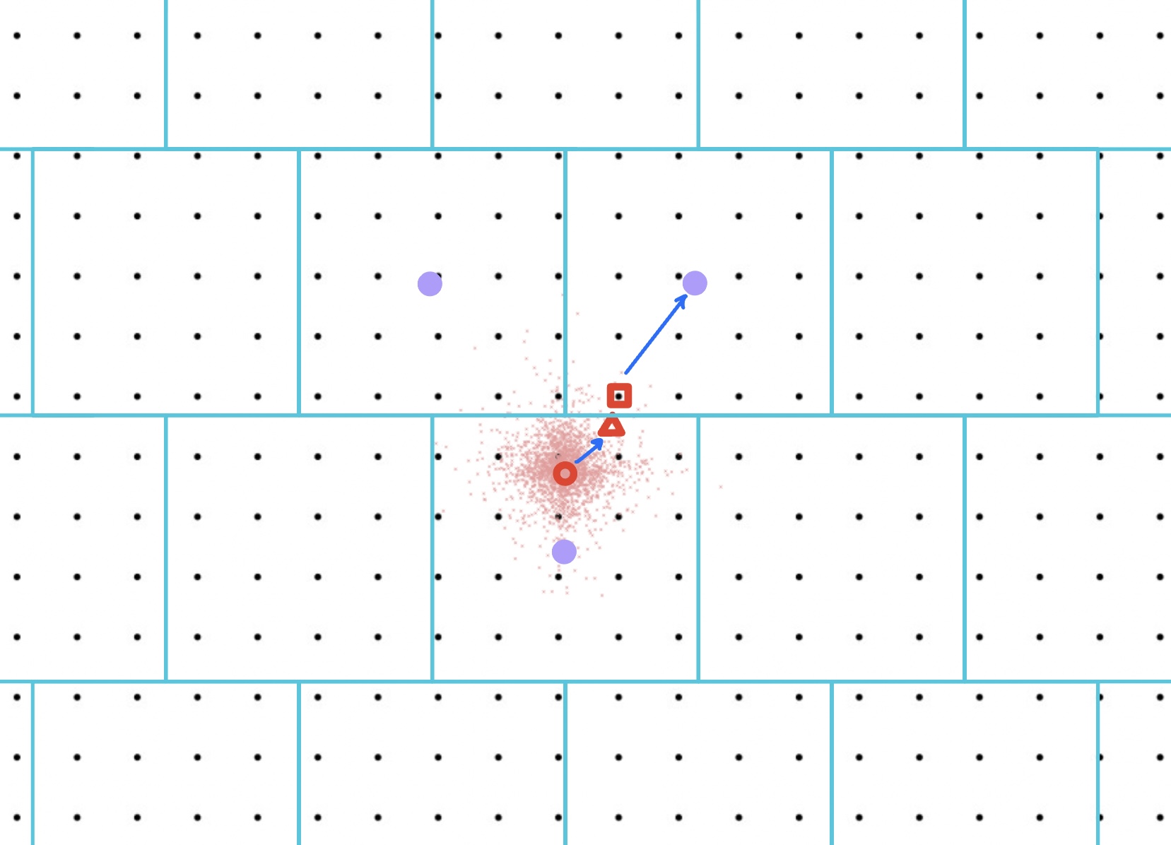It follows that $\operatorname{sum}(x^{(v)})=v$ , and if $u, v$ are at $\ell_{1}$ distance at most $a$ , then $x^{(u)}$ and $x^{(v)}$ are at distance at most $a$ from each other as datasets: $D_{\mathrm{Ham}}(x^{(u)},x^{(v)})\leq{\lVert u-v{\rVert}}_{1}$ .

Since $H_{\infty}(M)\leq\log_{2}K$ , for every $v\in G$ , there is some output $y^{(v)}\in\mathbb{R}^{d}$ such that $\Pr[M(x^{(v)})=y^{(v)}]\geq 1/K$ . (If there are several such outputs, choose the lexicographically largest.)

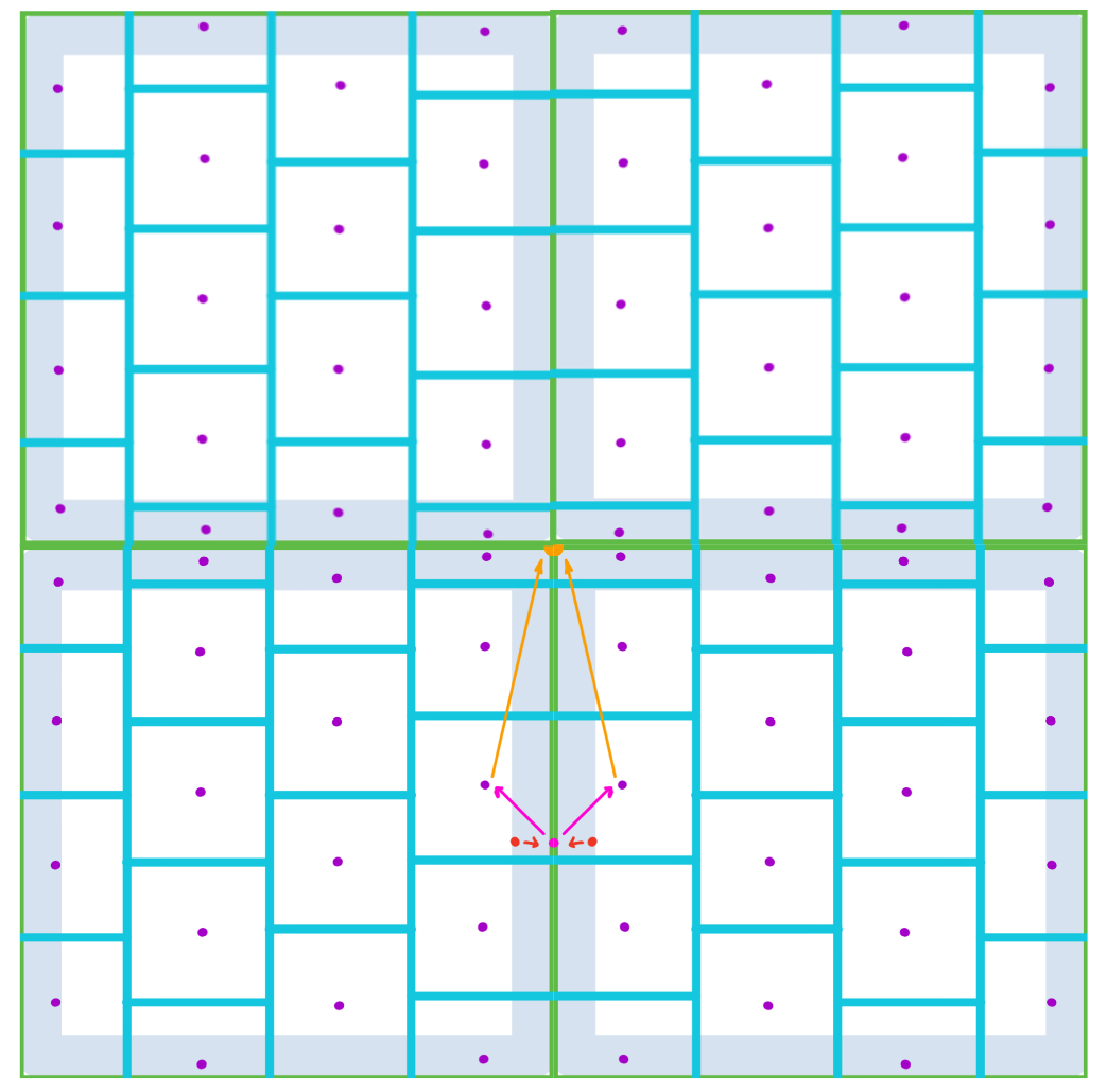
Now we construct our function $f\colon[0,1]^{d}\to\mathbb{R}^{d}$ as follows. For every $z\in[0,1]^{d}$ , let $v=v(z)$ be a point in $G$ obtained by rounding all coordinates of ${2(\alpha+1)}\cdot z$ to the nearest integer (and rounding up if halfway between integers). The resulting $v$ is in $G$ because ${2(\alpha+1)}\leq n$ , and by construction $v$ is at $\ell_{\infty}$ distance at most $1/2$ from ${2(\alpha+1)}\cdot z$ . Then $y^{(v)}$ exists as noted above. See Figure 3. Set

f(z)=y^{(v)}/{(2\alpha+2)}.

To show that $f$ is a deterministic rounding scheme, we analyze the two properties separately.

$\blacksquare$

To show that $\|f(z)-z\|_{\infty}\leq\rho<1/2$ , we use the accuracy of the mechanism. Fix any $z\in[0,1]^{d}$ : by construction, ${2(\alpha+1)}\cdot z$ and $v=v(z)$ are at $\ell_{\infty}$ distance at most $1/2$ . Recall that we have

$\Pr[{\lVert M(x^{(v)})-\operatorname{sum}(x^{(v)}){\rVert}}_{\infty}>\alpha]% \leq\beta,$

and

$\Pr[M(x^{(v)})=y^{(v)}]\geq\frac{1}{K}.$

Since $\beta<1/K$ , the outcome of $M(x^{(v)})$ has probability at most $1/K$ of being farther than $\alpha$ from $\operatorname{sum}(x^{(v)})$ . Since the particular outcome $y^{(v)}$ has probability greater than $1/K$ , then $y^{(v)}$ must be at $\ell_{\infty}$ distance at most $\alpha$ from $\operatorname{sum}(x^{(v)})=v$ , and hence at $\ell_{\infty}$ distance at most $\alpha+1/2$ from ${2(\alpha+1)}\cdot z$ . Hence, $f(z)=y^{(v)}/({2\alpha+2})$ is at $\ell_{\infty}$ distance at most $\rho={\frac{1}{2\alpha+2}\cdot\frac{2\alpha+1}{2}<\frac{1}{2}}$ from $z$ .
$\blacksquare$

For the second, we use the privacy guarantee of the mechanism: consider a closed $\ell_{\infty}$ ball $B(w,\tau^{\prime})$ and points $z_{1},\ldots,z_{k}\in B(w,\tau^{\prime})$ such that there are $k$ distinct outputs $f(z_{1}),\ldots,f(z_{k})$ . Let $v_{1},\ldots,v_{k}$ be the corresponding gridpoints, i.e., $v_{i}=v(z_{i})$ . Recall that $f(z_{i})=y^{(v_{i})}/({2\alpha+2})$ , so the $y^{(v_{i})}$ ’s are all distinct.

Since $z_{1},\ldots,z_{k}$ are all in $B(w,\tau^{\prime})$ , the gridpoints $v_{1},\ldots,v_{k}$ are all at $\ell_{\infty}$ distance at most ${2(\alpha+1)}\tau^{\prime}+1/2$ from ${2(\alpha+1)}w$ , which is itself at $\ell_{\infty}$ distance at most $1/2$ from some gridpoint $v_{0}$ . In particular, each $v_{i}$ is at $\ell_{1}$ distance at most $d\cdot({2(\alpha+1)}\tau^{\prime}+1)$ from $v_{0}$ , so the dataset $x^{(v_{i})}$ is at distance at most $h$ from $x^{(v_{0})}$ in Hamming distance, for

$h=\min(d\cdot({2(\alpha+1)}\tau^{\prime}+1),n).$

By (group) differential privacy, for each $1\leq i\leq k$ , we have

$\Pr[M(x^{(v_{0})})=y^{(v_{i})}]\geq e^{-\varepsilon\cdot h}\cdot\Pr[M(x^{(v_{i% })})=y^{(v_{i})}]-he^{(h-1)\varepsilon}\delta\geq e^{-\varepsilon\cdot h}\cdot% \frac{1}{K}-he^{-\varepsilon}\delta.$

Summing over $1\leq i\leq k$ , we get

$1\geq\sum_{i=1}^{k}\Pr[M(x^{(v_{0})})=y^{(v_{i})}]\geq e^{-\varepsilon\cdot h}% \cdot\frac{k}{K}-khe^{-\varepsilon}\delta.$

Reorganizing and upper bounding $e^{-\varepsilon}\leq 1$ , we have

$k\leq\frac{K\cdot e^{\varepsilon h}}{1-hKe^{h\varepsilon}\delta}$

as desired.

As mentioned earlier, all that remains is to invoke Lemma 4.3 to lift our deterministic rounding scheme from $[0,1]^{d}$ to the whole of $\mathbb{R}^{d}$ . $\hfill\blacktriangleleft$

It only remains to establish Lemma 4.3.

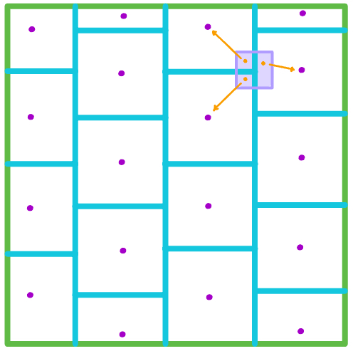
Proof of Lemma 4.3.

Fix a $(k,\tau)$ -deterministic rounding scheme $f\colon[0,1]^{d}\to\mathbb{R}^{d}$ of radius $\rho<1/2$ , with $\tau<1$ . Although the image of $f$ might extend to points outside $[0,1]^{d}$ by $\ell_{\infty}$ -distance $\rho<1/2$ , we may assume without loss of generality that the image of $f$ is contained in $[0,1]^{d}$ because projecting the outputs of $f$ to the nearest point in $[0,1]^{d}$ preserves both properties of a deterministic rounding scheme.

We first modify $f$ so that it behaves nicely near the faces of the cube to get a rounding scheme $f^{\prime}$ , then we show how to extend that to all of $\mathbb{R}^{d}$ to get the desired rounding scheme $f^{\prime\prime}$ .

We define $f^{\prime}\colon[0,1]^{d}\to[0,1]^{d}$ by the following process, which is also illustrated in Figure 4.

1.

Given $x\in[0,1]^{d}$ , for each $i\in[d]$ , set

$x^{\prime}_{i}=\begin{cases}0&\text{if $x_{i}\leq\tau/2$}\\ 1&\text{if $x_{i}\geq 1-\tau/2$}\\ x_{i}&\text{otherwise.}\end{cases}$

That is, if $x$ is in a “moat” of width $\tau/2$ , then it is $\tau/2$ -close to one (or possibly several) face(s) of the cube and $x^{\prime}$ is the projection of $x$ onto (the intersection of) the face(s). Otherwise, set $x^{\prime}=x$ . Note that $x^{\prime}$ is well-defined by our assumption that $\tau<1$ .
2.

For each $i\in[d]$ , set

$y_{i}=\begin{cases}0&\text{if $0\leq f(x^{\prime})_{i}<\frac{1}{2}$}\\ 1&\text{if $\frac{1}{2}\leq f(x^{\prime})_{i}\leq 1$.}\\ \end{cases}$

(Recall that we can assume without loss of generality that the image of $f$ is in $[0,1]^{d}$ .) That is, we round $f(x^{\prime})$ to the nearest corner of the cube.
3.

Set $f^{\prime}(x):=(y_{1},\ldots,y_{d})\in\mathbb{R}^{d}$ .

To understand the radius of $f^{\prime}$ , consider Figure 4. The first step from $x$ to $x^{\prime}$ is bounded (in $\ell_{\infty}$ distance) by $\tau/2$ (and is zero if $x$ is not in the moat). The second step from $x^{\prime}$ to $f(x^{\prime})$ is bounded by $\rho$ (the radius of $f$ ). The third step from $f(x^{\prime})$ to $y$ is bounded by $1/2$ (since it is rounding to a cube corner). The triangle inequality shows the total distance from $x$ to $y$ is bounded by $1/2+\rho+\tau/2$ , but Figure 4 suggests we can improve this bound: some cancellation is occurring in axes directions where $x$ is close to the boundary. To make this intuition precise, we do casework.

$\blacksquare$

If $x_{i}\leq\tau/2$ or $x_{i}\geq 1-\tau/2$ , then since $|f(x^{\prime})_{i}-x^{\prime}_{i}|\leq\rho<1/2$ , we see from $y_{i}$ ’s definition that $y_{i}=x^{\prime}_{i}$ so that

$|y_{i}-x_{i}|=|x^{\prime}_{i}-x_{i}|\leq\frac{\tau}{2}.$
$\blacksquare$

If $\tau/2<x_{i}<1-\tau/2$ , then since $y_{i}\in\{0,1\}$ , we have

$|y_{i}-x_{i}|<1-\frac{\tau}{2}.$

But when $\tau/2<x_{i}<1-\tau/2$ we also have $x^{\prime}_{i}=x_{i}$ , which implies that

$|y_{i}-x_{i}|\leq|(y_{i}-f(x^{\prime})_{i})|+|f(x^{\prime})_{i}-x^{\prime}_{i}% |\leq\frac{1}{2}+\rho.$

Since $\tau<1$ , the bound $\tau/2$ never exceeds either $1-\frac{\tau}{2}$ or $\frac{1}{2}+\rho$ . So, for all $x$ ,

{\lVert f^{\prime}(x)-x{\rVert}}_{\infty}\leq\min\!\left\{1-\frac{\tau}{2},% \frac{1}{2}+\rho\right\}\,,

establishing the bound on the radius.

Observe that for every $\ell_{\infty}$ ball $B_{\infty}(z,\tau/2)$ of radius $\tau/2$ , we have

|f^{\prime}(B_{\infty}(z,\tau/2)\cap[0,1]^{d})|\leq|f(B_{\infty}(z,\tau)\cap[0% ,1]^{d})|\leq k.

This is because if $\|x-z\|_{\infty}\leq\tau/2$ , then $\|x^{\prime}-z\|_{\infty}\leq\tau$ , and we obtain $f^{\prime}(x)$ by applying $f$ to $x^{\prime}$ and then projecting.

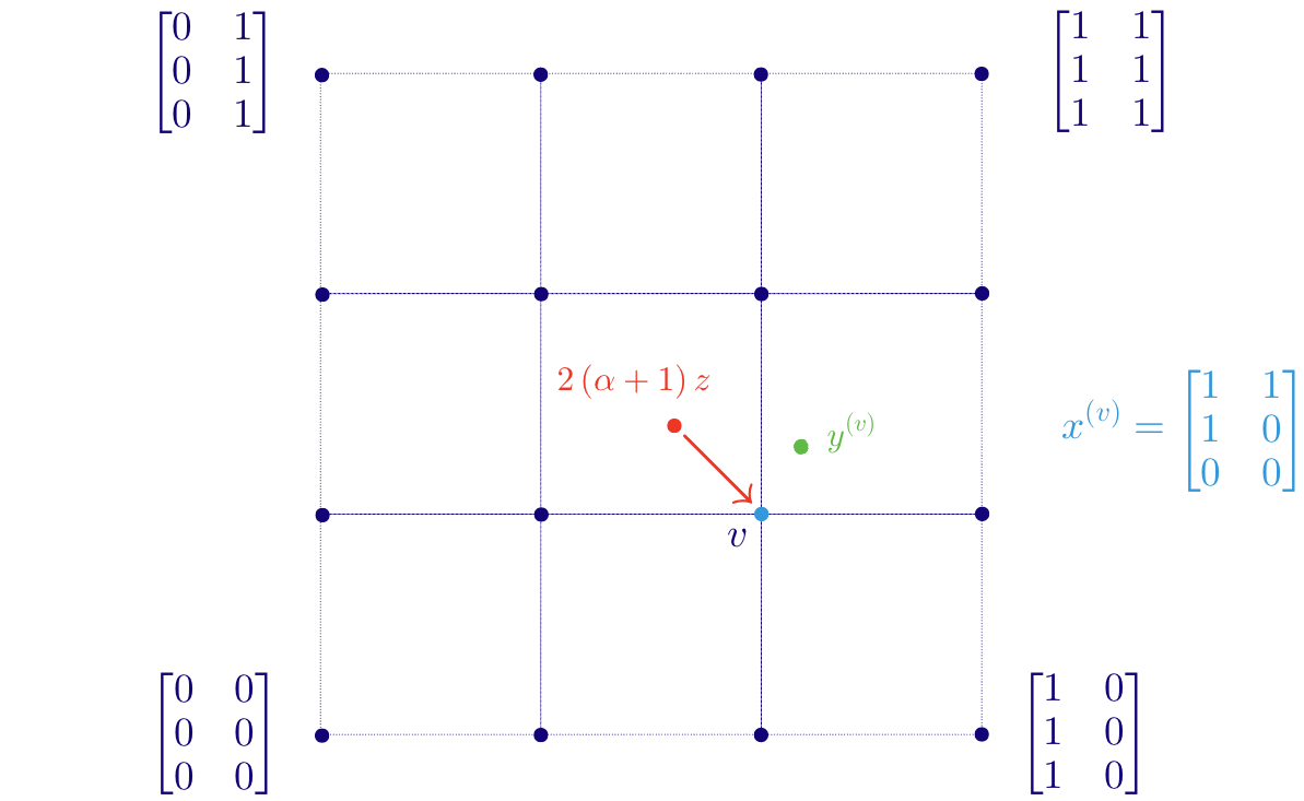
From $f^{\prime}$ , we construct a deterministic rounding scheme $f^{\prime\prime}\colon\mathbb{R}^{d}\to\mathbb{R}^{d}$ by using $f^{\prime}$ in each unit cube, but reflected so that points on either side of a unit cube boundary behave similarly. See Figure 5. We define $f^{\prime\prime}$ as follows:

Given $x\in\mathbb{R}^{d}$ .

1.

For each $i\in[d]$ , write $x_{i}=r_{i}+s_{i}e_{i}$ , where $r_{i}\in 2\mathbb{Z}$ , $s_{i}\in\{\pm 1\}$ , and $e_{i}\in[0,1]$ . Note that this is not unique when $x_{i}\in\mathbb{Z}$ , as two decompositions are then possible with either $s_{i}=1$ and one with $s_{i}=-1$ (but both with the same value of $e_{i}\in\{0,1\}$ ).⁵⁵5Specifically: if $x_{i}$ is an even integer, then $(r_{i},s_{i},e_{i})$ could be either $(x_{i},1,0)$ or $(x_{i},-1,0)$ . If $x_{i}$ is an odd integer, then the two options are $(x_{i}-1,1,1)$ and $(x_{i}+1,-1,1)$ . We will show that the output $f^{\prime\prime}(x)$ is independent of the choice we make.
2.

Let $e=(e_{1},\dots,e_{d})\in[0,1]^{d}$ .
3.

For each $i\in[d]$ , set $y_{i}=r_{i}+s_{i}f^{\prime}(e)_{i}$ .
4.

Set $f^{\prime\prime}(x)=(y_{1},\ldots,y_{d})$ .

The fact that $f^{\prime\prime}(x)$ is well-defined, regardless of the non-unique decompositions when $x_{i}$ is boolean follows from the facts that (a) the vector $e$ is independent of how those choices are made (already noted above), and (b) when $e_{i}\in\{0,1\}$ , we have $e^{\prime}_{i}=e_{i}$ and $f^{\prime}(e)_{i}=e^{\prime}_{i}$ (shown earlier for points $x$ where $x_{i}$ close to $0$ or $1$ ), so that $y_{i}=r_{i}+s_{i}f^{\prime}(e)_{i}=r_{i}+s_{i}e_{i}=x_{i}$ , regardless of whether we chose to use $s_{i}=1$ or $s_{i}=-1$ .

We can now analyze the guarantees this $f^{\prime\prime}$ provides. For every $x\in\mathbb{R}^{d}$ , since $|s_{i}|=1$ for all $i$ we get

{\lVert f^{\prime\prime}(x)-x{\rVert}}_{\infty}={\lVert f^{\prime}(e)-e{\rVert% }}_{\infty}\leq\min\left\{\frac{2-\tau}{2},\frac{1+2\rho}{2}\right\}

recalling the radius of $f^{\prime}$ established earlier. Next, consider any $\ell_{\infty}$ ball $B$ of radius at most $\tau/2$ . We claim that $|f^{\prime\prime}(B)|=|f^{\prime\prime}(B^{\prime})|$ for an $\ell_{\infty}$ ball $B^{\prime}\subseteq B$ that is entirely contained within a single unit hypercube whose corners are in $\mathbb{Z}^{d}$ , and thus $|f^{\prime\prime}(B^{\prime})|\leq k$ by the guarantees of $f^{\prime}$ . The reason is that if $x\in\mathbb{R}^{d}$ is within $\ell_{\infty}$ distance $\tau/2$ from a face $F$ of a unit hypercube, $f^{\prime\prime}(x)=f^{\prime\prime}(x^{\prime})$ , where $x^{\prime}$ is the projection of $x$ to $F$ . Thus we can remove portions of $B$ that are on the opposite side of a face from its center without changing $f(B)$ . (More formally, if we write $B=[a_{1},b_{1}]\times[a_{2},b_{2}]\times\cdots\times[a_{d},b_{d}]$ , then for any dimension $i$ where there is an integer $c_{i}$ strictly between $a_{i}$ and $b_{i}$ , we can replace the interval $[a_{i},b_{i}]$ with the shorter of $[a_{i},c_{i}]$ and $[c_{i},b_{i}]$ without changing $f(B).$ )

Therefore, $f^{\prime\prime}$ is a $(k,\zeta)$ -deterministic rounding scheme of radius $r=\min\!\left\{\frac{2-\tau}{2},\frac{1+2\rho}{2}\right\}$

\zeta=\frac{\tau/2}{2r}=\max\!\left\{\frac{\tau}{2(2-\tau)},\frac{\tau}{2(1+2% \rho)}\right\}.\

$\hfill\blacktriangleleft$

References

[1] Mark Bun, Marco Gaboardi, Max Hopkins, Russell Impagliazzo, Rex Lei, Toniann Pitassi, Satchit Sivakumar, and Jessica Sorrell. Stability is stable: Connections between replicability, privacy, and adaptive generalization. In Proceedings of the 55th Annual ACM Symposium on Theory of Computing, STOC 2023, pages 520–527, New York, NY, USA, 2023. Association for Computing Machinery. doi:10.1145/3564246.3585246.
[2] Mark Bun, Kobbi Nissim, Uri Stemmer, and Salil Vadhan. Differentially private release and learning of threshold functions. In Proceedings of the 56th Annual IEEE Symposium on Foundations of Computer Science (FOCS ‘15), pages 634–649. IEEE, 18–20 october 2015. Full version posted as arXiv:1504.07553. arXiv:1504.07553.
[3] Jesus A De Loera, Elisha Peterson, and Francis Edward Su. A polytopal generalization of Sperner’s lemma. Journal of Combinatorial Theory, Series A, 100(1):1–26, 2002. doi:10.1006/JCTA.2002.3274.
[4] Peter Dixon, A. Pavan, Jason Vander Woude, and N. V. Vinodchandran. List and certificate complexities in replicable learning. In Proceedings of the 37th International Conference on Neural Information Processing Systems (NeurIPS ‘23), NeurIPS ’23, Red Hook, NY, USA, 2023. Curran Associates Inc.
[5] Cynthia Dwork, Frank McSherry, Kobbi Nissim, and Adam Smith. Calibrating noise to sensitivity in private data analysis. In Theory of cryptography, volume 3876 of Lecture Notes in Comput. Sci., pages 265–284. Springer, Berlin, 2006. doi:10.1007/11681878_14.
[6] Cynthia Dwork and Aaron Roth. The algorithmic foundations of differential privacy. Found. Trends Theor. Comput. Sci., 9(3-4):211–407, 2014. doi:10.1561/0400000042.
[7] Simson L. Garfinkel and Philip Leclerc. Randomness concerns when deploying differential privacy. In WPES@CCS, pages 73–86. ACM, 2020. doi:10.1145/3411497.3420211.
[8] Badih Ghazi, Ravi Kumar, and Pasin Manurangsi. User-level differentially private learning via correlated sampling. In Marc’Aurelio Ranzato, Alina Beygelzimer, Yann N. Dauphin, Percy Liang, and Jennifer Wortman Vaughan, editors, Advances in Neural Information Processing Systems 34: Annual Conference on Neural Information Processing Systems 2021, NeurIPS 2021, December 6-14, 2021, virtual, pages 20172–20184, 2021. URL: https://proceedings.neurips.cc/paper/2021/hash/a89cf525e1d9f04d16ce31165e139a4b-Abstract.html.
[9] Ilya Mironov, Omkant Pandey, Omer Reingold, and Salil Vadhan. Computational differential privacy. In S. Halevi, editor, Advances in Cryptology—CRYPTO ‘09, volume 5677 of Lecture Notes in Computer Science, pages 126–142. Springer-Verlag, 16–20 august 2009. doi:10.1007/978-3-642-03356-8_8.
[10] Salil P. Vadhan. The complexity of differential privacy. In Tutorials on the Foundations of Cryptography, pages 347–450. Springer International Publishing, 2017. doi:10.1007/978-3-319-57048-8_7.
[11] Jason Vander Woude, Peter Dixon, Aduri Pavan, Jamie Radcliffe, and N. V. Vinodchandran. Geometry of rounding. CoRR, abs/2211.02694, 2022. doi:10.48550/arXiv.2211.02694.
[12] Jason Vander Woude, Peter Dixon, Aduri Pavan, Jamie Radcliffe, and N. V. Vinodchandran. Geometry of rounding: Near optimal bounds and a new neighborhood Sperner’s lemma. CoRR, abs/2304.04837, 2023. doi:10.48550/arXiv.2304.04837.

[bib.bib1] [1] Mark Bun, Marco Gaboardi, Max Hopkins, Russell Impagliazzo, Rex Lei, Toniann Pitassi, Satchit Sivakumar, and Jessica Sorrell. Stability is stable: Connections between replicability, privacy, and adaptive generalization. In Proceedings of the 55th Annual ACM Symposium on Theory of Computing, STOC 2023, pages 520–527, New York, NY, USA, 2023. Association for Computing Machinery. doi:10.1145/3564246.3585246.

[bib.bib2] [2] Mark Bun, Kobbi Nissim, Uri Stemmer, and Salil Vadhan. Differentially private release and learning of threshold functions. In Proceedings of the 56th Annual IEEE Symposium on Foundations of Computer Science (FOCS ‘15), pages 634–649. IEEE, 18–20 october 2015. Full version posted as arXiv:1504.07553. arXiv:1504.07553.

[bib.bib3] [3] Jesus A De Loera, Elisha Peterson, and Francis Edward Su. A polytopal generalization of Sperner’s lemma. Journal of Combinatorial Theory, Series A, 100(1):1–26, 2002. doi:10.1006/JCTA.2002.3274.

[bib.bib4] [4] Peter Dixon, A. Pavan, Jason Vander Woude, and N. V. Vinodchandran. List and certificate complexities in replicable learning. In Proceedings of the 37th International Conference on Neural Information Processing Systems (NeurIPS ‘23), NeurIPS ’23, Red Hook, NY, USA, 2023. Curran Associates Inc.

[bib.bib5] [5] Cynthia Dwork, Frank McSherry, Kobbi Nissim, and Adam Smith. Calibrating noise to sensitivity in private data analysis. In Theory of cryptography, volume 3876 of Lecture Notes in Comput. Sci., pages 265–284. Springer, Berlin, 2006. doi:10.1007/11681878_14.

[bib.bib6] [6] Cynthia Dwork and Aaron Roth. The algorithmic foundations of differential privacy. Found. Trends Theor. Comput. Sci., 9(3-4):211–407, 2014. doi:10.1561/0400000042.

[bib.bib7] [7] Simson L. Garfinkel and Philip Leclerc. Randomness concerns when deploying differential privacy. In WPES@CCS, pages 73–86. ACM, 2020. doi:10.1145/3411497.3420211.

[bib.bib8] [8] Badih Ghazi, Ravi Kumar, and Pasin Manurangsi. User-level differentially private learning via correlated sampling. In Marc’Aurelio Ranzato, Alina Beygelzimer, Yann N. Dauphin, Percy Liang, and Jennifer Wortman Vaughan, editors, Advances in Neural Information Processing Systems 34: Annual Conference on Neural Information Processing Systems 2021, NeurIPS 2021, December 6-14, 2021, virtual, pages 20172–20184, 2021. URL: https://proceedings.neurips.cc/paper/2021/hash/a89cf525e1d9f04d16ce31165e139a4b-Abstract.html.

[bib.bib9] [9] Ilya Mironov, Omkant Pandey, Omer Reingold, and Salil Vadhan. Computational differential privacy. In S. Halevi, editor, Advances in Cryptology—CRYPTO ‘09, volume 5677 of Lecture Notes in Computer Science, pages 126–142. Springer-Verlag, 16–20 august 2009. doi:10.1007/978-3-642-03356-8_8.

[bib.bib10] [10] Salil P. Vadhan. The complexity of differential privacy. In Tutorials on the Foundations of Cryptography, pages 347–450. Springer International Publishing, 2017. doi:10.1007/978-3-319-57048-8_7.

[bib.bib11] [11] Jason Vander Woude, Peter Dixon, Aduri Pavan, Jamie Radcliffe, and N. V. Vinodchandran. Geometry of rounding. CoRR, abs/2211.02694, 2022. doi:10.48550/arXiv.2211.02694.

[bib.bib12] [12] Jason Vander Woude, Peter Dixon, Aduri Pavan, Jamie Radcliffe, and N. V. Vinodchandran. Geometry of rounding: Near optimal bounds and a new neighborhood Sperner’s lemma. CoRR, abs/2304.04837, 2023. doi:10.48550/arXiv.2304.04837.

The Randomness Complexity of Differential Privacy

Abstract

Keywords and phrases:

Funding:

Copyright and License:

2012 ACM Subject Classification:

Related Version:

Acknowledgements:

DOI:

Event:

Editors:

Series and Publisher:

1 Introduction

Lemma 1.1.

Our results

Theorem 1.2 (Informal; see Corollary 3.2).

Theorem 1.3 (Informal; see Corollary 3.4).

Theorem 1.4 (Informal; see Corollary 4.2).

Connection to geometry

Related work on replicability

On using pseudorandom bits

Overview of the proofs

Directions for Future Work

2 Preliminaries

2.1 Differential Privacy

Definition 2.1 (Database metrics and adjacency).

Definition 2.2 (Differential privacy).

Definition 2.3 (Accuracy).

Lemma 2.4 (Postprocessing).

Lemma 2.5 (Group privacy).

Lemma 2.6 (Laplace mechanism; see e.g., [6, Theorems 3.6 and 3.8]).

Lemma 2.7 (Gaussian mechanism; see e.g., [6, Theorems 3.22 and A.1]).

2.2 Randomness Complexity

Definition 2.8 (randomness complexity).

Definition 2.9.

Lemma 2.10.

2.3 Deterministic Rounding Schemes and Secluded Partitions

Definition 2.11.

Theorem 2.12 ([11, 12]).

Theorem 2.13 ([11, 12]).

3 Upper bounds for summation

Theorem 3.1.

Corollary 3.2.

Proof of Theorem 3.1.

Mechanism 𝑴⁢(𝒙).

Theorem 3.3.

Corollary 3.4.

Proof Sketch of Theorem 3.3.

4 Lower bound for summation

Theorem 4.1.

Corollary 4.2.

Lemma 4.3.

Proof of Theorem 4.1.

Proof of Lemma 4.3.

Given 𝒙∈ℝ𝒅.

References

Mechanism $M(x)$ .

Given $x\in\mathbb{R}^{d}$ .