Extracting Dual Solutions via Primal Optimizers

Abstract
We provide a general method to convert a “primal” black-box algorithm for solving regularized convex-concave minimax optimization problems into an algorithm for solving the associated dual maximin optimization problem. Our method adds recursive regularization over a logarithmic number of rounds where each round consists of an approximate regularized primal optimization followed by the computation of a dual best response. We apply this result to obtain new state-of-the-art runtimes for solving matrix games in specific parameter regimes, obtain improved query complexity for solving the dual of the CVaR distributionally robust optimization (DRO) problem, and recover the optimal query complexity for finding a stationary point of a convex function.
Keywords and phrases:
Minimax optimization, black-box optimization, matrix games, distributionally robust optimizationFunding:
Yair Carmon: YC acknowledges support from the Israeli Science Foundation (ISF) grant no. 2486/21, and the Alon Fellowship.Copyright and License:
2012 ACM Subject Classification:
Theory of computation Mathematical optimizationEditor:
Raghu MekaSeries and Publisher:
1 Introduction
We consider the foundational problem of efficiently solving convex-concave games. For nonempty, closed, convex constraint sets and and differentiable convex-concave objective function (namely, is convex for any fixed and is concave for any fixed ), we consider the following primal, minimax optimization problem (P) and its associated dual, maximin optimization problem (D):
| (P) | ||||
| (D) |
If additionally and are bounded (which we assume for simplicity in the introduction but generalize later), every pair of primal and dual optimizers and satisfies the minimax principle: .
Convex-concave games are pervasive in algorithm design, machine learning, data analysis, and optimization. For example, the games induced by bilinear objectives, i.e., , where and are either the simplex, , or the Euclidean ball, , encompass zero-sum games, linear programming, hard-margin support vector machines (SVMs), and minimum enclosing/maximum inscribed ball [14, 2, 31, 10]. Additionally, the case when for some functions and is a subset of the simplex encompasses a variety of distributionally robust optimization (DRO) problems [29, 5] and (for ) the problem of minimizing the maximum loss [6, 8, 4].
In this paper, we study the following question:
Given only a black-box oracle which solves (regularized versions of) (P) to accuracy, and a black-box oracle for computing an exact dual best response to any primal point , can we extract an -optimal solution to (D)?
We develop a general dual-extraction framework which answers this question in the affirmative. We show that as long as these oracles can be implemented as cheaply as obtaining an -optimal point of (P), then our framework can obtain an -optimal point of (D) at the same cost as that of obtaining an -optimal point of (P), up to logarithmic factors. We then instantiate our framework to obtain new state-of-the-art results in the settings of bilinear matrix games and DRO. Finally, as evidence of its broader applicability, we show that our framework can be used to recover the optimal complexity for computing a stationary point of a smooth convex function.
In the remainder of the introduction we describe our results in greater detail (Section 1.1), give an overview of the dual extraction framework and its analysis (Section 1.2), discuss related work (Section 1.3), and provide a roadmap for the remainder of the paper (Section 1.4).
1.1 Our results
From primal algorithms to dual optimization
We give a general framework which obtains an -optimal solution to (D) via a sequence of calls to two black-box oracles: (i) an oracle for obtaining an -optimal point of a regularized version of (P), and (ii) an oracle for obtaining a dual best response for a given . In particular, we show it is always possible to obtain an -optimal point to (D) with at most a logarithmic number of calls to each of these oracles, where the regularized primal optimization oracle is always called to an accuracy of over a logarithmic factor. We also provide an alternate scheme (or more specifically choice of parameters) for applications where the cost of obtaining an -optimal point of the regularized primal problem decreases sufficiently as the regularization level increases. In such cases, e.g., in our stationary point application, it is possible to avoid even logarithmic factor increases in computational complexity for approximately solving (D) relative to the complexity of approximately solving (P).
Application 1: Bilinear matrix games
In this application, for a matrix , is the simplex , and is either the simplex or the unit Euclidean ball . Recently, [8] gave a new state-of-the-art runtime in certain parameter regimes of for obtaining an expected -optimal point for the primal problem (P) for this setup. However, unlike previous algorithms for bilinear matrix games (see Section 1.3 for details), their algorithm does not return an -optimal solution for the dual (D), and their runtime is not symmetric in the dimensions and . As a result, it was unclear whether the same runtime is achievable for obtaining an -optimal solution of the dual (D). We resolve this question by applying our general framework to achieve an expected -optimal point of (D) with runtime . We then observe (see Corollary 22) that in the setting where , our result can equivalently be viewed as a new state-of-the-art runtime of for obtaining an -optimal point of the primal (P) due to the symmetry of and the constraint sets.
Application 2: CVaR at level DRO
In this application, for convex, bounded, and Lipschitz loss functions , is a convex, compact set, and is the CVaR at level uncertainty set for . The primal (P) is a canonical and well-studied DRO problem, and corresponds to the average of the top fraction of the losses. We consider this problem given access to a first-order oracle that, when queried at and , outputs . Ignoring dependencies other than , the target accuracy , and the number of losses for brevity, [29] gave a matching upper and lower bound (up to logarithmic factors) of queries to obtain an expected -optimal point of the primal (P). However, the best known query complexity for obtaining an expected -optimal point of the dual (D) was prior to this paper (see Section 1.3 for details). Applying our general framework to this setting, we obtain an algorithm with a new state-of-the-art query complexity of for obtaining an expected -optimal point of the dual (D). In particular, note that this complexity is nearly linear in when .
Application 3: Obtaining stationary points of convex functions
In this application, we show that our framework yields an alternative optimal approach for computing an approximate critical point of a smooth convex function given a gradient oracle. Specifically, for and convex and -smooth , in Section 5, we give an algorithm which computes such that using gradient queries, where is the initial suboptimalityf. While this optimal complexity has been achieved before [24, 37, 15, 28, 27], that we achieve it is a consequence of our general framework illustrates its broad applicability.
For this application, we instantiate our framework with , where denotes the convex conjugate of . (For reasons discussed in Section 5, we actually first substitute for an appropriately regularized version of , call it , before applying the framework, but the following discussion still holds with respect to .) This objective function is known as the Fenchel game and has been used in the past to recover classic convex optimization algorithms (e.g., the Frank-Wolfe algorithm and Nesterov’s accelerated methods) via a minimax framework [1, 43, 12, 23]. In the Fenchel game, a dual best response corresponds to a gradient evaluation:
and we show that approximately optimal points for the dual objective (D) must have small norm. As a result, obtaining an approximately optimal dual point as a best response to a primal point yields a bound on the norm of . Furthermore, we note that in this setting, adding regularization to with respect to an appropriate choice of distance-generating function (namely ) is equivalent to rescaling and recentering the primal function , as well as the point at which a gradient is taken in the dual best response computation (cf. Lemma 14 in the full version). Thus, the properties of the Fenchel game extend naturally to appropriately regularized versions of .
1.2 Overview of the framework and analysis
We now give an overview of the dual-extraction framework. Our framework applies generally to a set of assumptions given in Section 3.1 (cf. Definition 9), but for now we specialize to the assumptions given above, namely: (i) the constraint sets and are nonempty, compact, and convex; and (ii) is differentiable and convex-concave. Throughout this section, let denote any norm on and assume that the dual function, , is -Lipschitz with respect to .111This is a weak assumption since we ensure at most a logarithmic dependence on ; see Remark 5. Let denote a differentiable distance-generating function (dgf) which is -strongly convex with respect to for ,222Section 2 gives the general setup for a distance-generating function which also covers the case where . and let denote the associated Bregman divergence. For the sake of illustration, it may be helpful to consider the choices , , , and in the following, in which case relative strong convexity with respect to is equivalent to the standard notion of strong convexity with respect to .
How should we obtain an -optimal point for (D) using the two oracles discussed previously, namely: (i) an oracle for approximately solving a regularized primal objective, and (ii) an oracle for computing a dual best response? We call (i) a dual-regularized primal optimization (DRPO) oracle and (ii) a dual-regularized best response (DRBR) oracle; their formal definitions are given in Section 3.1. Note that to solve (D), one cannot simply solve the primal problem (P) to high accuracy and then compute a dual best response. Consider with ; clearly , but for any arbitrarily close to , the dual best response is either or .
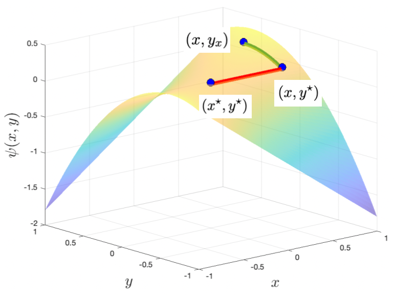
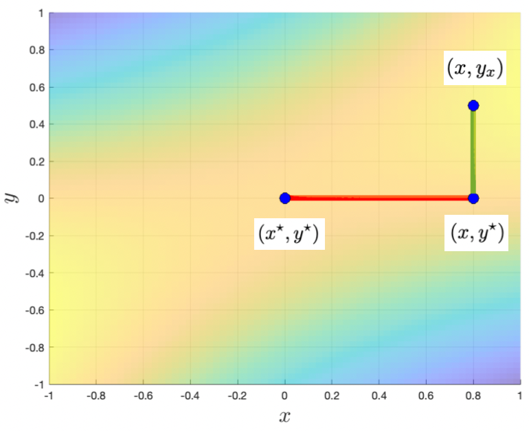
The key observation underlying our framework is that if is strongly concave for a given , it is possible to upper bound the distance between the best response and the dual optimum in terms of the primal suboptimality of . Figure 1 illustrates why this should be the case when subtracting a quadratic regularizer in (so that is strongly concave) to the preceding example of . We generalize this intuition in the following lemma (replacing strong concavity with relative strong concavity and a distance bound with a divergence bound), which is itself generalized further and proven in Section 3:
Lemma 1 (Lemma 3 from the full version specialized).
For a given , suppose is -strongly convex relative to the dgf for some . Then satisfies
A first try
In particular, Lemma 1 suggests the following approach: Define “dual-regularized” versions of as follows for and :
(Here, the subscript 1 denotes one level of regularization and will be extended later.) For any , note that is -strongly convex relative to , in which case Lemma 1 applied to yields
| (1) |
for , , and . Then note
| (2) |
where the first inequality follows since pointwise. Then by the -Lipschitzness of and -strong convexity of , it is straightforward to bound the suboptimality of as
| (3) |
Consequently, an -optimal point for (D) can be obtained via our oracles as follows: Set , and use the DRPO oracle on the regularized primal problem to obtain such that
| (4) |
Then the best response to with respect to , namely , is -optimal by (3). However, a typical setting in our applications is , , and , in which case ensuring (4) requires solving the regularized primal problem to error.
Recursive regularization and the dual-extraction framework
To lower the accuracy requirements, we apply dual regularization recursively. A key issue with the preceding argument is that it required a nontrivial bound on . However, it provided us with a nontrivial bound on , the “level-one equivalent” of . This suggests solving to lower accuracy while still obtaining a bound on due to (1), and then adding regularization centered at with a larger value of . Indeed, our framework recursively repeats this process until the total regularization is large enough so that (a term similar to) the right-hand side of (3) can be bounded by , despite never needing to solve a regularized primal problem to high accuracy.
To more precisely describe our approach, let . Over iterations , our framework implicitly constructs a sequence of convex-concave games , along with corresponding primal and dual functions and respectively, as follows:
| (5) | ||||
Here, is a dual-regularization schedule given as input to the framework, and is a sequence of dual-regularization “centers” generated by the algorithm, with given as input. For , it will be useful to let denote a maximizer of over and denote a minimizer of over , with and in particular.
Over the rounds of recursive dual regularization, we aim to balance two goals:
-
On the one hand, we want to increase quickly so that is very strongly convex relative to , thereby allowing us to apply Lemma 1 with a larger strong convexity constant.
-
On the other hand, we want to maintain the invariant that, roughly speaking, is always -optimal for the original dual . Indeed, we were constrained in choosing in (2) to be on the order of to ensure is -optimal for . A similar “constraint” on the dual-regularization schedule appears when (2) is extended to additional levels of regularization. This prevents us from increasing too quickly.
In all the applications in this paper we choose . typically must remain on the order of due to the second point.
Pseudocode of the framework is given in Algorithm 1. Each successive dual-regularization center is computed via the DRBR oracle (Line 5) as a best response to a primal point obtained via the DRPO oracle (Line 4). In Section 3, we generalize Algorithm 1 (cf. Algorithm 2) in several ways: (i) we allow for stochasticity in the DRPO oracle; (ii) we allow for distance-generating functions such that ; (iii) we give different but equivalent characterizations of and which facilitate the derivation of explicit expressions for the DRPO and DRBR oracles in applications.
Analysis of Algorithm 1
Theorem 2 is our main result for Algorithm 1. We then instantiate Theorem 2 with two illustrative choices of parameters in Corollaries 5 and 7, and defer the proofs of the latter to their general versions in Section 3. All of the remarks below (Remarks 3, 5, 7) are stated with reference to the specialized results in this section (Theorem 2 and Corollaries 4, 6 resp.), but extend immediately to the corresponding general versions (Theorem 15 and Corollaries 16, 17 resp.).
Theorem 2 (Theorem 15 specialized).
Algorithm 1 returns satisfying
| (6) |
and is a point with dual suboptimality bounded as
| (7) |
If we additionally assume that is -Lipschitz with respect to , we can directly bound the suboptimality of as
| (8) |
Proof.
We claim the first half of Theorem 2 holds with . To see this, note that we can bound the suboptimality of as
where follows since pointwise, follows from repeating the argument in the previous lines recursively (starting by lower bounding , etc.), and uses Lemma 1 applied to , which yields by Lines 4 and 5 in Algorithm 1:
since is -strongly concave relative to . Thus, we have proven Equation 7, and Equation 6 follows again from Lemma 1 applied to . Equation 8 then follows since the fact that is -strongly convex with respect to and Equation 6 imply
We give a remark regarding how to pick the parameters and when applying Theorem 2:
Remark 3 (Picking the parameters for Theorem 2).
Equation 8 can be interpreted as follows: To ensure is -optimal for , it suffices to choose the sequences and so that the right side of (8) is at most . Then the first term, , constrains to be on the order of . Skipping ahead, the third term, , is the reason we always choose in our applications, as this ensures is large enough to handle this term with only needing to be logarithmic in the problem parameters. Then the second term, , effectively constrains roughly , as .
Corollary 4 (Corollary 16 specialized).
Suppose is -Lipschitz with respect to , and let be such that . Then for any , and , the output of Algorithm 1 with dual-regularization and primal-accuracy schedules of
satisfies .
Remark 5.
Corollary 4 achieves the stated goal of obtaining an -optimal point for (D) by running for a number of iterations which depends logarithmically on the problem parameters, and solving each dual-regularized primal subproblem to an accuracy of divided by a logarithmic factor. Note in particular the logarithmic dependence on the dual divergence bound and dual Lipschitz constant , meaning these are weak assumptions. Furthermore, it is clear from the proof of Theorem 2 that only need be -Lipschitz on a set containing and .
Corollary 6 (Corollary 17 specialized).
Let be such that . Then for any and , the output of Algorithm 1 with dual-regularization and primal-accuracy schedules of
satisfies
where is a point whose suboptimality is at most , i.e., .
Remark 7.
Later calls to the DRPO oracle during the run of Algorithm 1 may be cheaper since there will be a significant amount of dual regularization at that point (namely, is large). One can sometimes take advantage of this (in particular, if the cost of a DRPO oracle call scales inverse polynomially with the regularization) to design schedules that avoid even the typically additional multiplicative logarithmic cost of Corollary 4 over the cost of a single DRPO oracle call. In such cases, a choice of schedules similar to those of Corollary 6 is often appropriate. With this choice of schedules, later rounds require very high accuracy. However, if one can argue that the increasing dual regularization makes the DRPO oracle call cheaper at a faster rate than the decreasing error makes it more expensive (as we do in Section 5), the total cost of applying the framework may collapse geometrically to the cost of a single DRPO oracle call made with target error approximately .
1.3 Related work
Black-box reductions
Our main contribution can be viewed as a black-box reduction from (regularized) primal optimization to dual optimization. Similar black-box reductions exist in the optimization literature. For example, [3] develops reductions between various fundamental classes of optimization problems, e.g., strongly convex optimization and smooth optimization. In a similar vein, the line of work [30, 18, 7] reduces convex optimization to approximate proximal point computation (i.e., regularized minimization).
Bilinear matrix games
Consider the bilinear objective where and are either the simplex, , or the Euclidean ball, . State-of-the-art methods in regard to runtime for obtaining an approximately optimal primal and/or dual solution can be divided into second-order interior point methods [11, 42] and stochastic first-order methods [22, 10, 9, 8]; see Table 2 in [8] for a summary of the best known runtimes as well as other references. Of importance to this paper, all state-of-the-art algorithms other than that of [8] are either (i) primal-dual algorithms which return both an -optimal primal and dual solution simultaneously, and/or (ii) achieve runtimes which are symmetric in the primal dimension and dual dimension , meaning the cost of obtaining an -optimal dual solution is the same as that of obtaining an -optimal primal solution. The algorithm of [8], on the other hand, only returns an -optimal primal point and further has a runtime which is not symmetric in and (see the footnote on the first page of that paper). As a result, solving the dual by simply swapping the roles of the primal and dual variables may be more expensive than solving the primal. (In fact, swapping the variables in this way may not even always be possible without further modifications due to restrictions on the constraint sets.)
CVaR at level distributionally robust optimization (DRO)
The DRO objectives we study are of the form , where the functions are convex, bounded, and Lipschitz, and , known as the uncertainty set, is a subset of the simplex. This objective corresponds to a robust version of the empirical risk minimization (ERM) objective where instead of taking an average over the losses (namely, is fixed at ), larger losses may be given more weight. In particular, in this paper we focus on a canonical DRO setting, CVaR at level , where the uncertainty set is given by for a choice of . CVaR DRO, along with its generalization -divergence DRO, has been of significant interest over the past decade; see [29, 5, 13, 32, 16] and the references therein. [29] is the most relevant to this paper – omitting parameters other than , the number of losses , and the target accuracy , they give a matching upper and lower bound (up to logarithmic factors) of first-order queries of the form to obtain an expected -optimal point of the primal objective. Their upper bound is achieved by a stochastic gradient method where the gradient estimator is based on a multilevel Monte Carlo (MLMC) scheme [19, 20]. However, the best known complexity for obtaining an expected -optimal point of the dual of CVaR at level is via a primal-dual method based on [33]; see also [13, 32] as well as [5, Appendix A.1], the last of which obtains complexity in the more general setting of the uncertainty set being an -divergence ball.
Stationary point computation
For , convex and -smooth with global minimum , and initialization point , consider the problem of computing a point such that . Two worst-case optimal gradient query complexities for this problem exist in the literature: and . An algorithm (the OGM-G method) which achieves the former complexity was given in [24], and [37] pointed out that any algorithm which achieves the former complexity can achieve the latter complexity. This is obtainable by running iterations of any optimal gradient method for reducing the function value, followed by iterations of a method which achieves the former complexity for reducing the gradient magnitude. In what may be of independent interest, we observe in Section 5.1 that a reduction in the opposite direction is also possible. More broadly, algorithms and frameworks for reducing the gradient magnitude of convex functions have been of much recent interest, and further algorithms and related work for this problem include [25, 27, 26, 28, 15, 37, 21], with lower bounds given in [34, 35].
1.4 Paper organization
In Section 2, we go over notation and conventions for the rest of the paper. We give our general dual-extraction framework and its guarantees in Section 3. In Section 4, we apply our framework to bilinear matrix games and the CVaR at level DRO problem. Finally, in Section 5 we give an optimal algorithm (in terms of query complexity) for computing an approximate stationary point of a convex and -smooth function.
2 Notation and conventions
We defer standard notation and conventions to the full version, and only include paper-specific notation here.
For , we use the notation for a fixed to denote the map (and define analogously). When we say satisfies a property, we mean it satisfies that property for any fixed (and analogously for ). We let , , and . In the latter two definitions, we may drop the superscript if it is clear from context, the argument if it is 0, and the subscript if it is 1. For , we may use either the notation or to denote its -th entry. denotes the all-ones vector. For a function which depends on some inputs , we write to denote the fact that is uniformly bounded above by a polynomial in as vary. We use the notation for the convex or Fenchel conjugate of . For , we let denote the infinite indicator of , namely if and if . For a function initially defined on a strict subset , we may implicitly extend the domain of to all of via its indicator as without additional comment. For a function with , we let denote the restriction of to . We note that denotes the convex conjugate of (and not restricted to ).
Following [38, Sec. 6.4], we encapsulate the setup for a dgf as follows. See the full version for additional discussion of this definition.
Definition 8 (dgf setup).
We say is a dgf setup over for closed and convex sets with if: (i) the distance-generating function (dgf) is convex and continuous over , differentiable on , and -strongly convex with respect to the chosen norm on for some ; and (ii) either or .
For a given dgf setup, we define its induced Bregman divergence for , and drop the superscript when it is clear from context.
3 Dual-extraction framework
In this section, we provide our general dual-extraction framework and its guarantees. In Section 3.1, we give the general setup, oracle definitions, and assumptions with which we apply and analyze the framework. Section 3.2 contains the statement and guarantees of the framework and Section 3.3 in the full version contains the associated proofs.
3.1 Preliminaries
We bundle all of the inputs to our framework into what we call a dual-extraction setup, defined below. Recall that when we say satisfies a property, we mean it satisfies that property for any fixed (and analogously for ).
Definition 9 (Dual-extraction setup).
A dual-extraction setup is a tuple where:
-
1.
is differentiable;
-
2.
and are convex and concave respectively;
-
3.
is a dgf setup over per Definition 8;
-
4.
the constraint sets and are nonempty, closed, and convex with and ;
-
5.
is bounded or is strongly convex;
-
6.
is bounded or is strongly concave;
-
7.
over all and , the map is constant over .333In all of our applications, this map will in fact be constant over .
Assumption 1 is only used in the proofs of Lemma 3 in the full version (the general version of Lemma 1 from Section 1.2) and Corollary 13 in the full version (used to show the framework is well-defined when ). Assumptions 2, 5, and 6 ensure that the minimax optimization problem with objective and constraint sets and satisfies the minimax principle; see below. Regarding Assumptions 3, 4, and 3, the fact that is potentially a strict subset of as well as the necessity of the technical assumption 3 is discussed in Remark 4 in the full version. In particular, Assumption 3 is only used to derive an equivalent formulation of the framework to Algorithm 1 which often allows for easier instantiations in applications, but is not strictly necessary to obtain our guarantees.
While our main results are stated in the full generality of Definition 9, in our applications we only particularize to Definition 10 and Definition 11 introduced below.
Definition 10 (Unbounded setup).
A -unbounded setup is a
-dual-extraction setup.
In other words, in an unbounded setup we choose and the Euclidean norm, in which case the dgf can be any differentiable and strongly convex function with respect to . Note that Assumption 3 is trivial as for all .
Definition 11 (Simplex setup).
A -simplex setup is a -dual-extraction setup where (with ).
In other words, in a simplex setup we choose , , we are using the -norm, and the dgf is negative entropy when restricted to the simplex. It is a standard result known as Pinsker’s inequality that is 1-strongly convex over with respect to , and the associated Bregman divergence is given by the Kullback-Leibler (KL) divergence for and . We verify that Assumption 3 holds in Appendix A.1 in the full version.
Notation associated with a setup
Whenever we instantiate a dual-extraction setup (Definition 9), we use the following notation and oracles associated with that setup without additional comment. We define the associated primal and dual functions, along with their corresponding primal and dual optimization problems, as they were introduced above in (P) and (D). We let and denote arbitrary primal and dual optima. To facilitate the discussion of dual-regularized problems, we define as follows
The minimax principle
Oracle definitions
Our framework assumes black-box access to , , and via a dual-regularized primal optimization (DRPO) oracle and a dual-regularized dual best response (DRBR) oracle defined below. Note that we generalize the setting of Section 1.2 by allowing the DRPO oracle to return an expected -optimal point; this is used in our applications in Section 4.
Definition 12 (DRPO oracle).
A -dual-regularized primal optimization oracle, , returns an expected -minimizer of , i.e., a point such that , where the expectation is over the internal randomness of the oracle.
Definition 13 (DRBR oracle).
A -dual-regularized best response oracle, , returns .
We also define a version of the DRPO oracle, called the DRPOSP oracle, which allows for a failure probability. We include this definition here due to its generality and broad applicability, but it is only used in Section 4.1 since the external result we cite to obtain an expected -minimizer of in that application has a failure probability. We also show in Appendix A.4 in the full version how to boost the success probability of a DRPOSP oracle.
Definition 14 (DRPOSP oracle).
A -dual-regularized primal optimization oracle with success probability, , returns an expected -minimizer of with success probability at least , where the expectation and success probability are over the internal randomness of the oracle.
3.2 The framework and its guarantees
We now state the general dual-extraction framework, Algorithm 2, and its guarantees, with proofs in the next section. As mentioned in Section 1.2, Algorithm 2 generalizes Algorithm 1 in three major ways: (i) we allow for stochasticity in the DRPO oracle; (ii) we allow for distance-generating functions where ; and (iii) we give different but equivalent characterizations of and which often allow for easier instantiations of the framework.
Regarding (iii), consider the case where the DRPO oracle is deterministic and for the sake of discussion. Note that in this case, the definitions of and in Lines 4 and 5 of Algorithm 2 may seem different than those in Lines 4 and 5 of Algorithm 1 at first glance. In particular, in Line 4 of Algorithm 2 is an -minimizer of over , whereas in Line 4 of Algorithm 1 is an -minimizer of over . Similarly, in Line 5 of Algorithm 2, whereas in Line 5 of Algorithm 1. In fact, we show in Section 3.3 in the full version that these are equivalent; see Lemma 2 and Remark 4 in the full version. The potential advantage of the expressions in Algorithm 2 compared to those in Algorithm 1 is that they involve only a single regularization term.
Note also that Line 3 of Algorithm 2 gives two equivalent expressions for the iterate ; their equivalence is proven in Appendix A.2 in the full version. Also, note that Line 4 is the only potential source of randomness in Algorithm 2; in particular, and are deterministic upon conditioning on . Finally, we show that Algorithm 2 is well-defined in Appendix A.3 in the full version; in particular, whenever a Bregman divergence is written in Algorithm 2, it is the case that . For example, in the context of a simplex setup per Definition 11, this corresponds to .
Theorem 15 (Algorithm 2 guarantee).
With calls to a DRPO oracle and calls to a DRBR oracle, Algorithm 2 returns satisfying
where is a point with expected suboptimality bounded as
If we additionally assume that is -Lipschitz with respect to , the expected suboptimality of can be directly bounded as
| (9) |
We now particularize Theorem 15 using two exemplary choices of the dual-regularization and primal-accuracy schedules. See Remarks 5 and 7 for additional comments.
Corollary 16.
Suppose is -Lipschitz with respect to , and let be such that . Then for any , and , the output of Algorithm 2 with dual-regularization and primal-accuracy schedules given by
satisfies .
Corollary 17.
Let be such that . Then for any and , the output of Algorithm 2 with dual-regularization and primal-accuracy schedules given by
| (10) |
satisfies
where is a point whose expected suboptimality is at most , i.e., .
4 Efficient maximin algorithms
In this section, we obtain new state-of-the-art runtimes for solving bilinear matrix games in certain parameter regimes (Section 4.1), as well as an improved query complexity for solving the dual of the CVaR at level distributionally robust optimization (DRO) problem (Section 4.2). In each application, we apply Corollary 16 to compute an -optimal point for the dual problem at approximately the same cost as computing an -optimal point for the primal problem (up to logarithmic factors and the cost of representing a dual vector when it comes to CVaR at level ).
4.1 Bilinear matrix games
In this section, we instantiate for a matrix . Given , we write , and use the notation , , and for the entry, -th row as a row vector, and -th column as a column vector. We consider two setups:
Definition 18 (Matrix games ball setup).
In the matrix games ball setup, we set (the unit Euclidean ball in ), , and fix a -simplex setup (Definition 11). We assume .
Definition 19 (Matrix games simplex setup).
In the matrix games simplex setup, we set , , and fix a -simplex setup (Definition 11). We assume .
Throughout Section 4.1, any theorem, statement, or equation which does not make reference to a specific choice of Definition 18 or 19 applies to both setups. Specializing the primal (P) and dual (D) to this application gives
| (P-MG) | ||||
| (D-MG) |
Regarding the assumptions on the norm of the matrix in Definitions 18 and 19, note that we can equivalently write with . Then the assumptions on the norm of correspond to ensuring is 1-Lipschitz with respect to the -norm in Definition 18 and -norm in Definition 19 (which in turn implies is 1-Lipschitz in the respective norms). This normalization is performed to simplify expressions as in [8]. (In particular, [8] also considers the more general problem where each can be any smooth, Lipschitz, convex function.)
Recently, [8, Cor. 8.2] achieved a state-of-the-art runtime in certain parameter regimes of for obtaining an -optimal point for (P-MG). However, unlike previous algorithms for (P-MG) (see Section 1.3 for an extended discussion), their algorithm does not yield an -optimal point for (D-MG) with the same runtime.
Our instantiation of the dual-extraction framework in Algorithm 3 and the accompanying guarantee Theorem 21 resolves this asymmetry between the complexity of obtaining a primal versus dual -optimal point by obtaining an -optimal point of (D-MG) with the same runtime of . At the end of Section 4.1, we observe that Theorem 21 also yields a new state-of-the-art runtime for the primal (P-MG) in the setting of Definition 19 due to the symmetry of the constraint sets and .
Before giving the guarantee Theorem 21 for Algorithm 3, the following lemma provides a runtime bound for the DRPOSP oracle when the success probability is (see Appendix B.1 in the full version for the proof). In particular, Lemma 20 shows that adding dual regularization to (P-MG) does not increase the complexity of obtaining an -optimal point over the guarantee of [8, Cor. 8.2] discussed above.
Lemma 20 (DRPOSP oracle for matrix games).
Now for the main guarantee (we defer the proof to the full version):
Theorem 21 (Guarantee for Algorithm 3).
The primal perspective
As alluded to above, the guarantee of Theorem 21 also implies a new state-of-the-art runtime for the primal (P-MG) in the setting of Definition 19. This follows because in the matrix games simplex setup, (P-MG) and (D-MG) are symmetric in terms of their constraint sets, so we can obtain an expected -optimal point for (P-MG) via Theorem 21 by negating and treating (P-MG) as if it were the dual problem. Formally (we defer the proof to the full version):
Corollary 22 (Guarantee for (P-MG) in the matrix games simplex setup).
See the full version for a discussion of how this runtime compares to the prior art.
4.2 CVaR at level DRO
In this section, we instantiate for convex, bounded, and -Lipschitz (with respect to the Euclidean norm) functions .444Note that we do not require the functions to be differentiable. Here, it is important that Definition 9 only requires to be differentiable. Given a compact, convex set and , the primal and dual problem for CVaR at level are as follows (we explain the reason for the notation as opposed to in the full version; in short, we apply the framework to a proxy objective):
| (P-CVaR) | ||||
| (D-CVaR) |
Our complexity model in this section is the number of computations of the form for and . We refer to the evaluation of for a given and as a single first-order query. Omitting the Lipschitz constant and bounds on the range of the ’s and size of for clarity, [29, Sec. 4] gave an algorithm which returns an expected555To be precise, [29] gives a -complexity high probability bound in Theorem 2. They do not state a -complexity expected suboptimality bound explicitly in a theorem, but they note in the text above Theorem 2 that such a bound follows immediately from Propositions 3 and 4 in their paper. -optimal point of (P-CVaR) with first-order queries, and also proved a matching lower bound up to logarithmic factors when is sufficiently large. However, to the best of our knowledge, the best known complexity for obtaining an expected -optimal point of (D-CVaR) is via a primal-dual method based on [33]; see also [13, 32, 5]. In our main guarantee for this section, Theorem 24, we apply Algorithm 2 to obtain an expected -optimal point of (D-CVaR) with complexity , which always improves upon or matches since .
Toward stating our main guarantee, we encapsulate the formal assumptions of [29, Sec. 2] in the following definition:
Definition 23 (CVaR at level setup).
We assume is nonempty, closed, convex, and satisfies for all . We also assume, for all , that is convex, -Lipschitz with respect to , and satisfies for all .
5 Obtaining critical points of convex functions
In this section, our goal is to obtain an approximate critical point of a convex, -smooth function , given access to a gradient oracle for . We show that our general framework yields an algorithm with the optimal query complexity for this problem. In Section 5.1, we give the formal problem definition and some important preliminaries. In Section 5.2, we give the setup for applying our main framework Algorithm 2 to this problem and a sketch of why the resulting algorithm works. In Section 5.3, we formally state the resulting algorithm for obtaining an approximate critical point of and prove that it achieves the optimal rate using the guarantees associated with Algorithm 2.
5.1 Preliminaries for Section 5
Throughout Section 5, we fix to be the standard Euclidean norm over . We assume is convex, -smooth with respect to , and for an arbitrary initialization point . We access through a gradient oracle. For , our goal will be to obtain a -critical point of , i.e., a point such that . Instead of operating on itself, our algorithm will operate on a regularized version of :
| (11) |
This notation was chosen to mirror the notation of Section 3.1; will be the primal function when we apply the framework. Let denote the unique global minimum of . The following corollary of Lemma 13 in Appendix C in the full version summarizes the key properties of :
Corollary 25 (Properties of the regularized function ).
We have
-
1.
.
-
2.
If is such that , then .
Proof.
This follows immediately from Lemma 13 in the full version with and .
The second part of Corollary 25 says that to find a -critical point of , it suffices to find a -critical point of . Furthermore, clearly a single query to suffices to obtain at a point. As a result, we will focus on finding a -critical point of . Furthermore, Corollary 25 may be of independent interest since it trivially allows one to achieve a gradient query complexity of via a method which achieves query complexity (for defined as some minimizer of over , assuming one exists); see Section 1.3.
The reason we perform this regularization before applying our framework is it enables us to obtain a sufficiently tight bound on (equivalently, a small enough value of when we ultimately apply Corollary 17). It is possible to apply the framework more directly to , but it is not clear how to do so in a way that achieves an optimal complexity.
5.2 Instantiating the framework
For this application, we instantiate
Recall that is the Fenchel game [1, 43, 12, 23]; see Section 1.1 for a discussion of why it is a natural choice in this setting. For the rest of Section 5, we fix a -unbounded setup (Definition 10) with . is a valid choice for the dgf because is differentiable and -strongly convex [38, Thm. 6.11]. The strong convexity of also implies that Assumption 6 holds. Note that the associated primal function is precisely (hence the choice of notation in (11)), and the dual function is given by
Next, the following lemma fulfills part of the outline given in Section 1.1 by showing that approximately optimal points for the dual objective (D) must have small norm. We defer the proof to the full version.
Lemma 26 (Bounding the norm by dual suboptimality).
If is -optimal for (D) for some , then .
We now derive the oracles of Definitions 12 and 13. Regarding Definition 12, for the rest of Section 5 we restrict to denote a deterministic implementation of the DRPO oracle, since we can always obtain a deterministic implementation in this application. Then the following corollary is an immediate consequence of a more general lemma given in Appendix C in the full version which characterizes the properties of the Fenchel game with added dual regularization; see also Section 1.1.
Corollary 27.
The set of valid output points of is precisely
Proof.
Apply Lemma 14 in the full version with .
Taken together, Lemma 26 and Corollary 27 nearly immediately imply that Algorithm 2 can be applied to the above setup to obtain a -critical point of (and therefore a -critical point of ). In particular, we will apply the schedules of Corollary 17 to certify that the output of Algorithm 2 is close in distance to an -optimal point for (D) for an appropriate choice of . Then Lemma 26 and a triangle inequality yield a bound on . Finally, since
by Corollary 27, we have that is an approximate critical point of (and therefore ). One may worry about the presence of here and, more generally, the presence of in the expressions for the oracles in Corollary 27. However, never needs to be evaluated explicitly since per the alternate expression for given in Line 3 of Algorithm 2, note that was itself computed as the gradient of at a point (recall the dgf is and ), in which case simply undoes this operation by Lemma 16 in the full version.
We formalize this sketch and provide a complexity guarantee in the next section. We also reframe this sketch and treat the sequence of terms as our iterates (as opposed to the sequence of ’s), as this leads to a simpler statement and interpretation of the resulting algorithm.
5.3 The resulting algorithm and guarantee
We now formalize the sketch given at the end of the previous section, state the resulting algorithm, and provide a complexity guarantee. But first, we define a subroutine which will be used by the algorithm to implement the DRPO oracle:
Definition 28 (CGM oracle [40, 36]).
A -fast composite gradient method oracle, , returns an -minimizer of over , i.e., an element of , using at most queries to .
For example, implementations with a small constant can be found in [40] or [36, Sec. 6.1.3]. The implementation of the CGM oracle falls under fast gradient methods for composite minimization, where letting denote a convex, -smooth function and a “simple regularizer” (a quadratic in our case), the goal is to minimize with the same complexity as it takes to minimize . The domain constraint can also be baked into the regularizer by adding an indicator.
Our method for computing a -critical point of is given in Algorithm 4, with the associated guarantee in Theorem 30. We note that the decision to introduce the equivalent notation for in Line 1 is aesthetic (to make Line 5 simpler to state and interpret). Furthermore, we state Algorithm 4 for general schedules and for clarity, but ultimately we will choose the schedules given in Theorem 30, which correspond to particularizing the schedules of Corollary 17 to this setting. With this choice of schedules, and so that . As a result, Algorithm 4 can be interpreted as optimizing in a sequence of balls where the radius and target error are both decreasing geometrically, and the center is a convex combination of the past iterates. While we choose the iteration count to be logarithmic in the problem parameters, we avoid multiplicative logarithmic factors in the total complexity because the ratio in the complexity of the CGM oracle call (to borrow the notation of Definition 28) in Line 5 of Algorithm 4 is at the -th iteration, meaning it is collapsing geometrically.
Toward analyzing Algorithm 4, we first connect the sequence of iterates produced by Algorithm 4 to the sequence of iterates produced by Algorithm 2 with the same input parameters. Namely, we are formalizing the comment made at the end of Section 5.2 about reframing the sequence of iterates to achieve a more interpretable algorithm. We defer the proof to the full version.
References
- [1] Jacob D Abernethy and Jun-Kun Wang. On frank-wolfe and equilibrium computation. In I. Guyon, U. Von Luxburg, S. Bengio, H. Wallach, R. Fergus, S. Vishwanathan, and R. Garnett, editors, Advances in Neural Information Processing Systems, volume 30. Curran Associates, Inc., 2017.
- [2] Ilan Adler. The equivalence of linear programs and zero-sum games. International Journal of Games Theory, Volume 42:165-177, February 2013.
- [3] Zeyuan Allen-Zhu and Elad Hazan. Optimal black-box reductions between optimization objectives. In Proceedings of the 30th International Conference on Neural Information Processing Systems, NIPS’16, pages 1614–1622, Red Hook, NY, USA, 2016. Curran Associates Inc.
- [4] Hilal Asi, Yair Carmon, Arun Jambulapati, Yujia Jin, and Aaron Sidford. Stochastic bias-reduced gradient methods. In Proceedings of the 35th International Conference on Neural Information Processing Systems, NIPS ’21, Red Hook, NY, USA, 2024. Curran Associates Inc.
- [5] Yair Carmon and Danielle Hausler. Distributionally robust optimization via ball oracle acceleration. In Proceedings of the 36th International Conference on Neural Information Processing Systems, NIPS ’22, Red Hook, NY, USA, 2024. Curran Associates Inc.
- [6] Yair Carmon, Arun Jambulapati, Yujia Jin, and Aaron Sidford. Thinking inside the ball: Near-optimal minimization of the maximal loss. In Mikhail Belkin and Samory Kpotufe, editors, Proceedings of Thirty Fourth Conference on Learning Theory, volume 134 of Proceedings of Machine Learning Research, pages 866–882. PMLR, 15–19 August 2021. URL: http://proceedings.mlr.press/v134/carmon21a.html.
- [7] Yair Carmon, Arun Jambulapati, Yujia Jin, and Aaron Sidford. Recapp: Crafting a more efficient catalyst for convex optimization. In International Conference on Machine Learning, 2022.
- [8] Yair Carmon, Arun Jambulapati, Yujia Jin, and Aaron Sidford. A Whole New Ball Game: A Primal Accelerated Method for Matrix Games and Minimizing the Maximum of Smooth Functions, pages 3685–3723. Society for Industrial and Applied Mathematics, 2024. doi:10.1137/1.9781611977912.130.
- [9] Yair Carmon, Yujia Jin, Aaron Sidford, and Kevin Tian. Variance reduction for matrix games. In H. Wallach, H. Larochelle, A. Beygelzimer, F. d'Alché-Buc, E. Fox, and R. Garnett, editors, Advances in Neural Information Processing Systems, volume 32. Curran Associates, Inc., 2019.
- [10] Kenneth L. Clarkson, Elad Hazan, and David P. Woodruff. Sublinear optimization for machine learning. J. ACM, 59(5), November 2012. doi:10.1145/2371656.2371658.
- [11] Michael B. Cohen, Yin Tat Lee, and Zhao Song. Solving linear programs in the current matrix multiplication time. In Proceedings of the 51st Annual ACM SIGACT Symposium on Theory of Computing, STOC 2019, pages 938–942, New York, NY, USA, 2019. Association for Computing Machinery. doi:10.1145/3313276.3316303.
- [12] Michael B. Cohen, Aaron Sidford, and Kevin Tian. Relative lipschitzness in extragradient methods and a direct recipe for acceleration. In James R. Lee, editor, 12th Innovations in Theoretical Computer Science Conference, ITCS 2021, January 6-8, 2021, Virtual Conference, volume 185 of LIPIcs, pages 62:1–62:18. Schloss Dagstuhl – Leibniz-Zentrum für Informatik, 2021. doi:10.4230/LIPICS.ITCS.2021.62.
- [13] Sebastian Curi, Kfir Y. Levy, Stefanie Jegelka, and Andreas Krause. Adaptive sampling for stochastic risk-averse learning. In Proceedings of the 34th International Conference on Neural Information Processing Systems, NIPS ’20, Red Hook, NY, USA, 2020. Curran Associates Inc.
- [14] G. B. Dantzig. Linear programming and extensions, 1953.
- [15] Jelena Diakonikolas and Puqian Wang. Potential function-based framework for minimizing gradients in convex and min-max optimization. SIAM Journal on Optimization, 32(3):1668–1697, 2022. doi:10.1137/21M1395302.
- [16] John Duchi and Hongseok Namkoong. Learning models with uniform performance via distributionally robust optimization. The Annals of Statistics, 49, June 2021.
- [17] I. Ekeland, Roger Temam, Society for Industrial, and Applied Mathematics. Convex analysis and variational problems. Classics in applied mathematics. Society for Industrial and Applied Mathematics (SIAM), Philadelphia, Pa., 1999.
- [18] Roy Frostig, Rong Ge, Sham M. Kakade, and Aaron Sidford. Un-regularizing: approximate proximal point and faster stochastic algorithms for empirical risk minimization. In Proceedings of the 32nd International Conference on International Conference on Machine Learning - Volume 37, ICML’15, pages 2540–2548. JMLR.org, 2015. URL: http://proceedings.mlr.press/v37/frostig15.html.
- [19] Michael B. Giles. Multilevel monte carlo path simulation. Operations Research, 56(3):607–617, June 2008. doi:10.1287/OPRE.1070.0496.
- [20] Michael B. Giles. Multilevel monte carlo methods. Acta Numerica, 24:259–328, May 2015. doi:10.1017/S096249291500001X.
- [21] G. N. Grapiglia and Yurii Nesterov. Tensor methods for finding approximate stationary points of convex functions. Optimization Methods and Software, 37(2):605–638, 2022. doi:10.1080/10556788.2020.1818082.
- [22] Michael D. Grigoriadis and Leonid G. Khachiyan. A sublinear-time randomized approximation algorithm for matrix games. Operations Research Letters, 18(2):53–58, 1995. doi:10.1016/0167-6377(95)00032-0.
- [23] Yujia Jin, Aaron Sidford, and Kevin Tian. Sharper rates for separable minimax and finite sum optimization via primal-dual extragradient methods. In Po-Ling Loh and Maxim Raginsky, editors, Proceedings of Thirty Fifth Conference on Learning Theory, volume 178 of Proceedings of Machine Learning Research, pages 4362–4415. PMLR, 02–05 July 2022. URL: https://proceedings.mlr.press/v178/jin22b.html.
- [24] Donghwan Kim and Jeffrey A. Fessler. Optimizing the efficiency of first-order methods for decreasing the gradient of smooth convex functions. Journal of Optimization Theory and Applications, 188(1):192–219, January 2021. doi:10.1007/S10957-020-01770-2.
- [25] Jaeyeon Kim, Asuman Ozdaglar, Chanwoo Park, and Ernest K. Ryu. Time-reversed dissipation induces duality between minimizing gradient norm and function value, 2023. arXiv:2305.06628.
- [26] Jaeyeon Kim, Chanwoo Park, Asuman Ozdaglar, Jelena Diakonikolas, and Ernest K. Ryu. Mirror duality in convex optimization, 2024. arXiv:2311.17296.
- [27] Guanghui Lan, Yuyuan Ouyang, and Zhe Zhang. Optimal and parameter-free gradient minimization methods for convex and nonconvex optimization, 2023. arXiv:2310.12139.
- [28] Jongmin Lee, Chanwoo Park, and Ernest K. Ryu. A geometric structure of acceleration and its role in making gradients small fast. In Neural Information Processing Systems, 2021.
- [29] Daniel Levy, Yair Carmon, John C Duchi, and Aaron Sidford. Large-scale methods for distributionally robust optimization. In H. Larochelle, M. Ranzato, R. Hadsell, M.F. Balcan, and H. Lin, editors, Advances in Neural Information Processing Systems, volume 33, pages 8847–8860. Curran Associates, Inc., 2020.
- [30] Hongzhou Lin, Julien Mairal, and Zaid Harchaoui. A universal catalyst for first-order optimization. In Proceedings of the 28th International Conference on Neural Information Processing Systems - Volume 2, NIPS’15, pages 3384–3392, Cambridge, MA, USA, 2015. MIT Press.
- [31] M. Minsky and S. Papert. Perceptrons: An introduction to computational geometry, 1988.
- [32] Hongseok Namkoong and John C. Duchi. Stochastic gradient methods for distributionally robust optimization with f-divergences. In Proceedings of the 30th International Conference on Neural Information Processing Systems, NIPS’16, pages 2216–2224, Red Hook, NY, USA, 2016. Curran Associates Inc.
- [33] A. Nemirovski, A. Juditsky, G. Lan, and A. Shapiro. Robust stochastic approximation approach to stochastic programming. SIAM Journal on Optimization, 19(4):1574–1609, 2009. doi:10.1137/070704277.
- [34] A.S Nemirovsky. On optimality of krylov’s information when solving linear operator equations. Journal of Complexity, 7(2):121–130, 1991. doi:10.1016/0885-064X(91)90001-E.
- [35] A.S Nemirovsky. Information-based complexity of linear operator equations. Journal of Complexity, 8(2):153–175, 1992. doi:10.1016/0885-064X(92)90013-2.
- [36] Yurii Nesterov. Lectures on Convex Optimization. Springer Publishing Company, Incorporated, 2nd edition, 2018.
- [37] Yurii Nesterov, Alexander Gasnikov, Sergey Guminov, and Pavel Dvurechensky. Primal-dual accelerated gradient methods with small-dimensional relaxation oracle. Optimization Methods and Software, 36(4):773–810, July 2021. doi:10.1080/10556788.2020.1731747.
- [38] Francesco Orabona. A modern introduction to online learning, 2023. arXiv 1912.13213. arXiv:1912.13213.
- [39] Maurice Sion. On general minimax theorems. Pacific Journal of Mathematics, 8:171–176, 1958.
- [40] Paul Tseng. On accelerated proximal gradient methods for convex-concave optimization, 2008.
- [41] J. v. Neumann. Zur theorie der gesellschaftsspiele. Mathematische Annalen, 100(1):295–320, December 1928.
- [42] Jan van den Brand, Yin Tat Lee, Yang P. Liu, Thatchaphol Saranurak, Aaron Sidford, Zhao Song, and Di Wang. Minimum cost flows, mdps, and -regression in nearly linear time for dense instances. In Proceedings of the 53rd Annual ACM SIGACT Symposium on Theory of Computing, STOC 2021, pages 859–869, New York, NY, USA, 2021. Association for Computing Machinery.
- [43] Jun-Kun Wang, Jacob Abernethy, and Kfir Y. Levy. No-regret dynamics in the fenchel game: a unified framework for algorithmic convex optimization. Mathematical Programming, 205(1-2):203–268, May 2024. doi:10.1007/S10107-023-01976-Y.