Unraveling Universally Closest Refinements via Symmetric Density Decomposition and Fisher Market Equilibrium

Chan, T-H. Hubert; Xue, Quan

doi:10.4230/LIPIcs.ITCS.2025.35

Unraveling Universally Closest Refinements via Symmetric Density Decomposition and Fisher Market Equilibrium

T-H. Hubert Chan

Department of Computer Science, University of Hong Kong, Hong Kong Quan Xue

Department of Computer Science, University of Hong Kong, Hong Kong

Abstract

We investigate the closest distribution refinements problem, which involves a vertex-weighted bipartite graph as input, where the vertex weights on each side sum to 1 and represent a probability distribution. A refinement of one side’s distribution is an edge distribution that corresponds to distributing the weight of each vertex from that side to its incident edges. The objective is to identify a pair of distribution refinements for both sides of the bipartite graph such that the two edge distributions are as close as possible with respect to a specific divergence notion. This problem is a generalization of transportation, in which the special case occurs when the two closest distributions are identical. The problem has recently emerged in the context of composing differentially oblivious mechanisms.

Our main result demonstrates that a universal refinement pair exists, which is simultaneously closest under all divergence notions that satisfy the data processing inequality. Since differential obliviousness can be examined using various divergence notions, such a universally closest refinement pair offers a powerful tool in relation to such applications.

We discover that this pair can be achieved via locally verifiable optimality conditions. Specifically, we observe that it is equivalent to the following problems, which have been traditionally studied in distinct research communities: (1) hypergraph density decomposition, and (2) symmetric Fisher Market equilibrium.

We adopt a symmetric perspective of hypergraph density decomposition, in which hyperedges and nodes play equivalent roles. This symmetric decomposition serves as a tool for deriving precise characterizations of optimal solutions for other problems and enables the application of algorithms from one problem to another. This connection allows existing algorithms for computing or approximating the Fisher market equilibrium to be adapted for all the aforementioned problems. For example, this approach allows the well-known iterative proportional response process to provide approximations for the corresponding problems with multiplicative error in distributed settings, whereas previously, only absolute error had been achieved in these contexts. Our study contributes to the understanding of various problems within a unified framework, which may serve as a foundation for connecting other problems in the future.

Keywords and phrases:

closest distribution refinements, density decomposition, Fisher market equilibrium

Funding:

T-H. Hubert Chan: This research was partially supported by the Hong Kong RGC grants 17201823, 17203122 and 17202121.

Copyright and License:

2012 ACM Subject Classification:

Mathematics of computing

\rightarrow

Distribution functions ; Theory of computation

\rightarrow

Mathematical optimization

Editors:

Raghu Meka

Series and Publisher:

Leibniz International Proceedings in Informatics, Schloss Dagstuhl – Leibniz-Zentrum für Informatik

1 Introduction

In this work, we explore several existing and new problems under the same unifying framework. By unraveling previously unknown connections between these seemingly unrelated problems, we offer deeper insights into them. Moreover, existing solutions for one problem can readily offer improvements to other problems. Input instances for these problems all have the following form.
Input Instance. An instance is a vertex-weighted bipartite graph with vertex bipartition $\mathcal{I}=\mathcal{I}^{(0)}\mathbin{\mathchoice{\leavevmode\vtop{\halign{% \hfil$\m@th\displaystyle#$\hfil\cr\cup\cr\cdot\crcr}}}{\leavevmode\vtop{% \halign{\hfil$\m@th\textstyle#$\hfil\cr\cup\cr\cdot\crcr}}}{\leavevmode\vtop{% \halign{\hfil$\m@th\scriptstyle#$\hfil\cr\cup\cr\cdot\crcr}}}{\leavevmode\vtop% {\halign{\hfil$\m@th\scriptscriptstyle#$\hfil\cr\cup\cr\cdot\crcr}}}}\mathcal{% I}^{(1)}$ , edge set $\mathcal{F}$ and positive¹¹1Vertices with zero weights are removed and identified with the empty set $\emptyset$ . vertex weights $w:\mathcal{I}\to\mathbb{R}_{>0}$ . For some problems, it is convenient to normalize the vertex weights into distributions, i.e., the vertex weights on each side sum to 1; in this case, we call this a distribution instance. We use $\mathbb{B}:=\{0,1\}$ to index the two sides. Given a side $\iota\in\mathbb{B}$ , we use $\overline{\iota}:=\iota\oplus 1$ to denote the other side.
Solution Concept. We shall see that in each problem, refinement is the underlying solution concept. Given a side $\iota\in\mathbb{B}$ , a refinement²²2Since vertex weights on one side can be interpreted as a probability distribution, allocating the weight of each vertex to its incident edges can be viewed as a refinement of the original distribution. $\alpha^{(\iota)}$ on vertex weights on side $\iota$ indicates how each vertex $i\in\mathcal{I}^{(\iota)}$ distributes its weight $w(i)$ among its incident edges in $\mathcal{F}$ . In other words, $\alpha^{(\iota)}$ is a vector of edge weights in $\mathcal{F}$ such that for each $i\in\mathcal{I}^{(\iota)}$ , the sum of weights of edges incident on $i$ equals $w(i)$ . While some problems may require refinements of vertex weights from one side only, it will still be insightful to consider a refinement pair $\vec{\alpha}=(\alpha^{(0)},\alpha^{(1)})$ of vertex weights on both sides.

The main problem we focus on is the closest distribution refinement problem, which we show is intricately related to other problems. In probability theory, a divergence notion quantifies how close two distributions are to each other, where a smaller quantity indicates that they are closer. Common examples of divergences include total variation distance and KL-divergence. Observe that a divergence notion ${\mathsf{D}}$ needs not be symmetric, i.e. for two distributions $P$ and $Q$ on the same sample space, it is possible that ${\mathsf{D}}(P\|Q)\neq{\mathsf{D}}(Q\|P)$ .

Definition 1 (Closest Distribution Refinement Problem).

Given a distribution instance $(\mathcal{I}^{(0)},\mathcal{I}^{(1)};\mathcal{F};w)$ and a divergence notion ${\mathsf{D}}$ , the goal is to find a distribution refinement pair $\vec{\alpha}=(\alpha^{(0)},\alpha^{(1)})$ such that the distributions $\alpha^{(0)}$ and $\alpha^{(1)}$ on the edges $\mathcal{F}$ are as close to each other as possible under ${\mathsf{D}}$ , i.e., ${\mathsf{D}}(\alpha^{(0)}\|\alpha^{(1)})$ is minimized.

Universally Closest Refinement Pair. It is not clear a priori if a refinement pair achieving the minimum for one divergence notion would also achieve the minimum for another divergence notion. For a non-symmetric divergence ${\mathsf{D}}$ , a pair $\vec{\alpha}=(\alpha^{(0)},\alpha^{(1)})$ minimizing ${\mathsf{D}}(\alpha^{(0)}\|\alpha^{(1)})$ may not necessarily achieve the minimum ${\mathsf{D}}(\alpha^{(1)}\|\alpha^{(0)})$ . The special case when $\vec{\alpha}$ consists of a pair of identical refinements is also known as $w$ -transportation or perfect fractional matching [9, 27, 34, 6], in which case $\vec{\alpha}$ is obviously the minimizer for all divergences.

In general, it would seem ambitious to request a universally closest refinement pair that simultaneously minimizes all “reasonable” divergence notions. In the literature, all commonly used divergence notions satisfy the data processing inequality, which intuitively says that the divergence of two distributions cannot increase after post-processing. Formally, for any deterministic function $\varphi:\Omega\to\widehat{\Omega}$ , the induced distribution $\varphi(P)$ and $\varphi(Q)$ on $\widehat{\Omega}$ satisfy the inequality: ${\mathsf{D}}(\varphi(P)\|\varphi(Q))\leq{\mathsf{D}}(P\|Q)$ . Surprisingly, we show that such a universally closest pair exists.

Theorem 2 (Universally Closest Refinement Pair).

Given a distribution instance $(\mathcal{I}^{(0)},\mathcal{I}^{(1)};\mathcal{F};w)$ , there exists a distribution refinement pair $\vec{\alpha}=(\alpha^{(0)},\alpha^{(1)})$ that minimizes ${\mathsf{D}}(\alpha^{(0)}\|\alpha^{(1)})$ simultaneously for all divergence notions ${\mathsf{D}}$ that satisfy the data processing inequality.

Moreover, this pair can be returned using the near-linear time algorithm of Chen et al. [14] for the minimum quadratic-cost flow problem.

Since Definition 1 gives a clean mathematical problem, we first describe the technical contributions and approaches of this work, and we describe its motivation and application in Section 1.2.

While the technical proofs are given in Sections 4 and 5, we give some motivation for why the problem is studied in the first place and sketch the key ideas for our proofs.

1.1 Our Technical Contributions and Approaches

In addition to the problem in Definition 1, we shall see that the following solution properties are also the key to solving other problems as well.
Desirable Solution Properties. Two desirable solution properties are local maximin and proportional response.

$\blacksquare$

Local Maximin. A refinement $\alpha^{(\iota)}$ on vertex weights on side $\iota$ can also be interpreted as how each vertex in $\mathcal{I}^{(\iota)}$ allocates its weight to its neighbors on the other side $\mathcal{I}^{(\overline{\iota})}$ via the edges in $\mathcal{F}$ . Specifically, for $i\in\mathcal{I}^{(\iota)}$ and $j\in\mathcal{I}^{(\overline{\iota})}$ , $\alpha^{(\iota)}(ij)$ is the payload received by $j$ from $i$ , where we rely on the superscript in $\alpha^{(\iota)}$ to indicate that the payload is sent from side $\iota$ to side $\overline{\iota}$ along an edge in $\mathcal{F}$ . Consequently, $\alpha^{(\iota)}$ induces a payload vector $p\in\mathbb{R}^{\mathcal{I}^{(\overline{\iota})}}$ , where $p(j)=\sum_{i}\alpha^{(\iota)}(ij)$ is the total payload received by $j$ in the allocation $\alpha^{(\iota)}$ . Recalling that vertex $j$ also has a weight, the payload density (resulting from $\alpha^{(\iota)}$ ) of $j$ is $\rho(j):=\frac{p(j)}{w(j)}$ .

The refinement $\alpha^{(\iota)}$ is locally maximin if for each $i\in\mathcal{I}^{(\iota)}$ , vertex $i$ distributes a non-zero payload $\alpha^{(\iota)}(ij)>0$ to vertex $j$ only if $j$ is among the neighbors of $i$ with minimum payload densities (resulting from $\alpha^{(\iota)}$ ).

The intuition of the term “maximin” is that vertex $i$ tries to maximize the minimum payload density among its neighbors by giving its weight to only neighbors that achieve the minimum payload density.
$\blacksquare$

Proportional Response. Given a refinement $\alpha^{(\iota)}$ on vertex weights on side $\iota$ , its proportional response $\alpha^{(\overline{\iota})}$ is a refinement on vertex weights from the other side $\overline{\iota}$ . Specifically, vertex $j\in\mathcal{I}^{(\overline{\iota})}$ distributes its weight $w(j)$ proportionately according to its received payloads: $\alpha^{(\overline{\iota})}(ij)=\frac{\alpha^{(\iota)}(ij)}{p(j)}\cdot w(j)$ .

Several problems in the literature studied in different contexts can be expressed with the same goal.

Goal 3 (High-Level Goal).

Given an instance $(\mathcal{I}^{(0)},\mathcal{I}^{(1)};\mathcal{F};w)$ , find a refinement pair $\vec{\alpha}=(\alpha^{(0)},\alpha^{(1)})$ such that both refinements are locally maximin and proportional response to each other.

This abstract problem have been studied extensively in the literature under different contexts, and various algorithms to exactly achieve or approximate (whose meaning we will explain) Goal 3 have been designed. One contribution of this work is to unify all these problems under our abstract framework. Consequently, we readily offer new approximation results for some problems that are unknown before this connection is discovered.

We next describe how our abstract framework is related to each considered problem and what new insights or results are achieved, which also provide the tools to solve or approximate the problem in Definition 1.

1.1.1 Hypergraph Density Decomposition

An instance $(\mathcal{I}^{(0)},\mathcal{I}^{(1)};\mathcal{F};w)$ is interpreted as a hypergraph $H$ . Each element in $i\in\mathcal{I}^{(0)}$ is a hyperedge and each element in $j\in\mathcal{I}^{(1)}$ is a node, where $\{i,j\}\in\mathcal{F}$ means that node $j$ is contained in hyperedge $i$ . Observe that in this hypergraph, both the hyperedges and the nodes are weighted.

Densest Subset Problem.

Given a subset $S\subseteq\mathcal{I}^{(1)}$ of nodes in a (weighted) hypergraph, its density is $\rho(S):=\frac{w(H[S])}{w(S)}$ , where $H[S]$ is the collection of hyperedges containing only nodes inside $S$ . The densest subset problem requests a subset $S$ with the maximum density.

Density Decomposition.

The decomposition can be described by an iterative process that generates a density vector $\rho_{*}\in\mathbb{R}^{\mathcal{I}^{(1)}}$ for the nodes in the hypergraph by repeated peeling off densest subsets. First, the (unique) maximal densest subset $S_{1}$ is obtained, and each $j\in S_{1}$ will be assigned the density $\rho_{*}(j)=\frac{w(H[S_{1}])}{w(S_{1})}$ of $S_{1}$ . Then, the hyperedges $H[S_{1}]$ and the subset $S_{1}$ are removed from the instance; note that any hyperedge containing a node outside $S_{1}$ will remain. The process is applied to the remaining instance until eventually every node in $\mathcal{I}^{(1)}$ is removed and assigned its density. The collection of subsets found in the iterative process forms the density decomposition $\mathcal{I}^{(1)}=\mathbin{\mathchoice{\leavevmode\vtop{\halign{\hfil$\m@th% \displaystyle#$\hfil\cr\cup\cr\cdot\crcr}}}{\leavevmode\vtop{\halign{\hfil$% \m@th\textstyle#$\hfil\cr\cup\cr\cdot\crcr}}}{\leavevmode\vtop{\halign{\hfil$% \m@th\scriptstyle#$\hfil\cr\cup\cr\cdot\crcr}}}{\leavevmode\vtop{\halign{\hfil% $\m@th\scriptscriptstyle#$\hfil\cr\cup\cr\cdot\crcr}}}}_{k\geq 1}S_{k}$ .

As mentioned in [22], the earliest variant of this decomposition was introduced by Fujishige [19] in the context of polymatroids. We describe the related work in more detail in Section 1.3.

Connection with the Local Maximin Condition.

Charikar [13] gave an LP (that can be easily generalized to weighted hypergraphs) which solves the densest subset problem exactly, and a refinement $\alpha^{(0)}$ on the weights of hyperedges $\mathcal{I}^{(0)}$ corresponds exactly to a feasible solution of the dual LP. Replacing the linear function in this dual LP with a quadratic function while keeping the same feasible variable $\alpha^{(0)}$ , Danisch et al. [15] considered a quadratic program (that has also appeared in [19]). They showed that a refinement corresponds to an optimal solution to the quadratic program iff it is locally maximin³³3Instead of using the term “maximin”, the same concept is called “stability” in [15].. Moreover, a locally maximin refinement also induces the aforementioned density vector $\rho_{*}$ .

As observed in [22], the quadratic program can be expressed as a minimum quadratic-cost flow problem, which can be solved optimally using the nearly-linear time algorithm of Chen et al. [14]. As we shall show that our considered problems are all equivalent to Goal 3, this implies the algorithmic result in Theorem 2.

Symmetry of Density Decomposition.

We observe that the density decomposition is symmetric between the hyperedges and the nodes. Recall that in iteration $k$ of the density decomposition, a subset $S_{k}$ is produced, together with its corresponding collection $\widehat{S}_{k}$ of hyperedges that determines the density $\frac{w(\widehat{S}_{k})}{w(S_{k})}$ . Therefore, in addition to a partition of nodes, there is a corresponding decomposition of the hyperedges $\mathcal{I}^{(0)}=\mathbin{\mathchoice{\leavevmode\vtop{\halign{\hfil$\m@th% \displaystyle#$\hfil\cr\cup\cr\cdot\crcr}}}{\leavevmode\vtop{\halign{\hfil$% \m@th\textstyle#$\hfil\cr\cup\cr\cdot\crcr}}}{\leavevmode\vtop{\halign{\hfil$% \m@th\scriptstyle#$\hfil\cr\cup\cr\cdot\crcr}}}{\leavevmode\vtop{\halign{\hfil% $\m@th\scriptscriptstyle#$\hfil\cr\cup\cr\cdot\crcr}}}}_{k\geq 1}\widehat{S}_{k}$ .

Given an abstract instance $(\mathcal{I}^{(0)},\mathcal{I}^{(1)};\mathcal{F};w)$ , one could have interpreted it differently with $\mathcal{I}^{(0)}$ as nodes and $\mathcal{I}^{(1)}$ as hyperedges. When the density decomposition is constructed with the roles reversed, the exact sequence $\{(\widehat{S}_{k},S_{k})\}_{k}$ of pairs is obtained, but in reversed order. Intuitively, $(\widehat{S}_{1},S_{1})$ is the densest from the perspective of $S_{1}\subseteq\mathcal{I}^{(1)}$ , but it is the least dense from the perspective of $\widehat{S}_{1}\subseteq\mathcal{I}^{(0)}$ .

The symmetric nature of the density decomposition has been mentioned recently by Harb et al. [23, Theorem 13], but we shall explain later this fact may be inferred when different earlier works are viewed together. Hence, this observation may be considered as part of the folklore. Since we need some crucial properties of the symmetric density decomposition to prove Theorem 2, for the sake of completeness, the connection of Goal 3 and this folklore result is described in Section 3.

Approximation Notions.

Even though the exact density decomposition can be achieved via LP or maximum flow, it can be computationally expensive in practice. In the literature, efficient approximation algorithms have been considered. While there are different attempts to define approximation notions for density decompositions, it is less clear what they mean when they are applied to different problems.

Observe that a refinement pair $\vec{\alpha}=(\alpha^{(0)},\alpha^{(1)})$ achieving Goal 3 may not be unique, but the induced payload vectors $(p^{(0)}_{*},p^{(1)}_{*})$ and density vectors $(\rho^{(0)}_{*},\rho^{(1)}_{*})$ are unique. When we say approximating Goal 3, we mean finding a refinement pair such that the induced payload and density vectors have some approximation guarantees. We shall see that approximation guarantees⁴⁴4See Definition 12 for approximation notions of muliplicative vs absolute errors on vectors. on these vectors can be translated readily to approximation notions for various problems.

1.1.2 Unraveling Universally Closest Distribution Refinements via Symmetric Density Decomposition

Restricted Class of Divergence.

As a first step towards proving Theorem 2, we consider a restricted class of divergences known as hockey-stick divergence. For each $\gamma\geq 0$ ,

\mathsf{D}_{\gamma}(P\|Q):=\sup_{S\subseteq\Omega}Q(S)-\gamma\cdot P(S).

The hockey-stick divergence is related to the well-known $(\epsilon,\delta)$ -differential privacy inequality. Specifically, $\mathsf{D}_{e^{\epsilon}}(P\|Q)\leq\delta$ iff for all subsets $S\subseteq\Omega$ ,

Q(S)\leq e^{\epsilon}\cdot P(S)+\delta.

We first consider the universal closest distribution refinements with respect to the class of hockey-stick divergences $\mathcal{D}_{\textrm{HS}}:=\{\mathsf{D}_{\gamma}:\gamma\geq 0\}$ . In Lemma 31, we show that the restricted variant of Theorem 2 to the class $\mathcal{D}_{\textrm{HS}}$ is equivalent to the following problem.

Universal Refinement Matching Problem.

Given an instance $G=(\mathcal{I}^{(0)},\mathcal{I}^{(1)};\mathcal{F};w)$ and two non-negative weights $\vec{c}=(c^{(0)},c^{(1)})\in\mathbb{R}^{\mathbb{B}}$ , we use $G^{(\vec{c})}$ to denote the instance of (fractional) maximum matching on the bipartite graph $(\mathcal{I}^{(0)},\mathcal{I}^{(1)};\mathcal{F})$ with vertex capacity constraints. For side $\iota$ and $i\in\mathcal{I}^{(\iota)}$ , the capacity constraint at vertex $i$ is $c^{(\iota)}\cdot w(i)$ . A fractional solution consists of assigning non-negative weights to the edges in $\mathcal{F}$ such that the weighted degree of every vertex does not exceed its capacity constraint. Observe that for any refinement pair $\vec{\alpha}=(\alpha^{(0)},\alpha^{(1)})$ , the fractional matching $\vec{c}\bullet\vec{\alpha}$ defined below is a feasible solution to $G^{(\vec{c})}$ :

\vec{c}\bullet\vec{\alpha}(ij):=\min\{c^{(0)}\cdot\alpha^{(0)}(ij),c^{(1)}% \cdot\alpha^{(1)}(ij)\}\text{ for all }\{i,j\}\in\mathcal{F}.

The goal is to find a refinement pair $\vec{\alpha}=(\alpha^{(0)},\alpha^{(1)})$ such that for any weight pair $\vec{c}$ , the edge weights $\vec{c}\bullet\vec{\alpha}$ form an optimal (fractional) solution to the maximum matching instance $G^{(\vec{c})}$ .

The structure of the symmetric density decomposition described in Section 1.1.1 makes it convenient to apply a primal-dual analysis to achieve the following in Section 4.

Theorem 4 (Universal Maximum Refinement Matching).

Given an instance $(\mathcal{I}^{(0)},\mathcal{I}^{(1)};\mathcal{F};w)$ , suppose a distribution refinement pair $\vec{\alpha}=(\alpha^{(0)},\alpha^{(1)})$ satisfies Goal 3. Then, for any $\vec{c}=(c^{(0)},c^{(1)})$ , the (fractional) solution $\vec{c}\bullet\vec{\alpha}$ is optimal for the maximum matching instance $G^{(\vec{c})}$ .

Extension to General Case.

To extend Theorem 2 beyond the restricted divergence class $\mathcal{D}_{\textrm{HS}}$ , we consider the closest distribution refinement problem under a more general probability distance notion.
Capturing All Data Processing Divergences via Power Functions. As opposed to using a single number by a divergence notion to measure the closeness of two distributions, the power function $\mathsf{Pow}(P\|Q):[0,1]\to[0,1]$ between distributions $P$ and $Q$ captures enough information to recover all divergence notions that satisfy the data processing inequality. We will give a formal explanation in Section 5. A main result is given in Theorem 37, which states that any distribution refinement pair satisfying Goal 3 achieves the minimal power function, from which Theorem 2 follows immediately.

Approximation Results.

In the full version [12], we show that a refinement that induces a payload with multiplicative error can lead to approximation guarantees for other problems. For the universal refinement matching problem, a natural approximation notion is based on the standard approximation ratio for the maximum matching problem.

On the other hand, achieving a meaningful approximation notion for the universally closest distribution refinement problem in terms of divergence values is more difficult. The reason is that any strictly increasing function on a data processing divergence still satisfies the data processing inequality. Therefore, any non-zero deviation from the correct answer may be magnified arbitrarily. Instead of giving approximation guarantees directly on the divergence values, we consider a technical notion of power function stretching, and the approximation quality of a refinement pair is quantified by how much the optimal power function is stretched. The formal statement is given in the full version [12].

1.1.3 Achieving Multiplicative Error via Proportional Response in Fisher Markets

We next interpret an instance $(\mathcal{I}^{(0)},\mathcal{I}^{(1)};\mathcal{F};w)$ as a special symmetric case of linear Fisher markets [18], which is itself a special case of the more general Arrow-Debreu markets [2]. This allows us to transfer any algorithmic results for Fisher/Arrow-Debreu market equilibrium to counterparts for Goal 3. Specifically, we can use a quick iterative procedure proportional response [39, 40] to approximate the densities of vertices in the density decomposition in Section 1.1.1 with multiplicative error, where only absolute error has been achieved before [15, 22]. In addition to being interesting in its own right, multiplicative error is also used to achieve the approximation results in Section 1.1.2.

Market Interpretation.

Even though in an instance, the roles of the two sides are symmetric, it will be intuitive to think of $\mathcal{I}^{(0)}$ as buyers and $\mathcal{I}^{(1)}$ as sellers. For buyer $i\in\mathcal{I}^{(0)}$ , the weight $w(i)$ is its budget. In the symmetric variant, the utilities of buyers have a special form. Each seller $j\in\mathcal{I}^{(1)}$ has one divisible unit of good $j$ for which a buyer $i$ has a positive utility exactly when $\{i,j\}\in\mathcal{F}$ , in which case the utility per unit of good $j$ is $w(j)$ (that is common for all buyers that have a positive utility for $j$ ). For a general Fisher market, a buyer $i$ can have an arbitrary utility $w_{i}(j)$ for one unit of good $j$ .
Market Allocation and Equilibrium. For the symmetric variant, an allocation can be represented by a refinement pair $\vec{\alpha}=(\alpha^{(0)},\alpha^{(1)})$ , in which $\alpha^{(1)}$ must be a proportional response to $\alpha^{(0)}$ . For the refinement $\alpha^{(0)}$ on the buyers’ budgets, the induced payload vector $p^{(1)}$ on the sellers corresponds to the price vector on goods. For the refinement $\alpha^{(1)}$ on the sellers’ weights, the induced payload vector $p^{(0)}$ on the buyers corresponds to the utilities received by the buyers. It is well-known (explained in the full version [12]) that a market equilibrium is characterized by a locally maximin refinement $\alpha^{(0)}$ of buyers’ budgets together with its proportional response $\alpha^{(1)}$ . From our theory of symmetric density decomposition in Section 1.1.1, this is equivalent to Goal 3.

Alternative Characterization.

The fact that the local maximin condition on the buyers’ budget allocation is equivalent to Fisher market equilibrium readily allows us to borrow any algorithmic results for market equilibrium to solve or approximate Goal 3. In the full version [12], we give details on the following observations.

$\blacksquare$

In linear Fisher markets (not necessarily symmetric), we show that the local maximin condition on sellers’ goods allocation to buyers can be used to characterize a market equilibrium. This is an alternative characterization of linear Fisher market equilibrium that involves only goods allocation and buyers’ utilities, but not involving good prices.
$\blacksquare$

On the other hand, we show that there exists an Arrow-Debreu market such that there is a goods allocation satisfying the local maximin condition, but it is not an equilibrium.

1.2 Motivation and Application for Universally Closest Distribution Refinements

The problem in Definition 26 arises in the study of the composition of differentially oblivious mechanisms [41, 42], which is a generalization of the more well-known concept of differential privacy (DP) [17].

A Quick Introduction to Differential Privacy/Obliviousness.

Consider a (randomized) mechanism $\mathcal{M}$ that takes an input from space $\mathcal{X}$ and returns an output from space $\mathcal{Y}$ that will be passed to a second mechanism. During the computation of $\mathcal{M}$ , an adversary can observe some view from space $\mathcal{V}$ that might not necessarily include the output in general. Suppose at first we just consider the privacy/obliviousness of $\mathcal{M}$ on its own, which measures how much information the adversary can learn about the input from its view. Intuitively, it should be difficult for the adversary to distinguish between two similar inputs from their corresponding views produced by the mechanism. Formally, similar inputs in $\mathcal{X}$ are captured by a neighboring symmetric relation, and the privacy/obliviousness of the mechanism $\mathcal{M}$ requires that the two distributions of views produced by neighboring inputs are “close”, where closeness can be quantified by some notion of divergence. As mentioned in Section 1.1.2, the popular notion of $(\epsilon,\delta)$ -DP is captured using hockey-stick divergences.

Composition of Differentially Oblivious Mechanisms.

Suppose the output of mechanism $\mathcal{M}$ from space $\mathcal{Y}$ is passed as an input to a second mechanism $\mathcal{M}^{\prime}$ , which is differentially oblivious with respect to some neighboring relation on $\mathcal{Y}$ . Hence, given input $x$ to $\mathcal{M}$ , one should consider the joint distribution $\mathcal{M}(x)$ on the space $\mathcal{V}\times\mathcal{Y}$ of views and outputs.

The notion of neighbor-preserving differential obliviousness (NPDO) has been introduced [41, 42] to give sufficient conditions on $\mathcal{M}$ that allows composition with such a mechanism $\mathcal{M}^{\prime}$ so that the overall composition preserves differential obliviousness.

Specifically, given neighboring inputs $x_{0}\sim x_{1}$ , conditions are specified on the two distributions $\mathcal{M}(x_{0})$ and $\mathcal{M}(x_{1})$ . Unlike the case for differential privacy/obliviousness, it is not appropriate to just require that the two distributions are close. This is because the adversary can only observe the view component of $\mathcal{V}\times\mathcal{Y}$ . Moreover, one also needs to incorporate the neighboring relation on the output space $\mathcal{Y}$ , which is needed for the privacy guarantee for the second mechanism $\mathcal{M}^{\prime}$ .

The definition of NPDO is more conveniently described via the terminology offered by our abstract instance $(\mathcal{I}^{(0)},\mathcal{I}^{(1)};\mathcal{F};w)$ . Here, the sets $\mathcal{I}^{(0)}$ and $\mathcal{I}^{(1)}$ are two copies of $\mathcal{V}\times\mathcal{Y}$ . For each $\iota\in\mathbb{B}$ , the weights $w$ on $\mathcal{I}^{(\iota)}$ corresponds to the distribution $\mathcal{M}(x_{\iota})$ . Finally, $(v_{0},y_{0})\in\mathcal{I}^{(0)}$ and $(v_{1},y_{1})\in\mathcal{I}^{(1)}$ are neighbors in $\mathcal{F}$ iff $v_{0}=v_{1}$ and $y_{0}\sim y_{1}$ are neighboring in $\mathcal{Y}$ .

In the original definition [42], the mechanism $\mathcal{M}$ is said to be $d$ -NPDO with respect to divergence $\mathsf{D}$ if for the constructed instance $(\mathcal{I}^{(0)},\mathcal{I}^{(1)};\mathcal{F};w)$ , there exists a distribution refinement pair $\vec{\alpha}=(\alpha^{(0)},\alpha^{(1)})$ , which may depend on the divergence $\mathsf{D}$ , such that $\mathsf{D}(\alpha^{(0)}\|\alpha^{(1)})\leq d$ . Examples of considered divergences include the standard hockey-stick divergence and Rényi divergence [31].

Since it only makes sense to consider divergences satisfying the data processing inequality in the privacy context, the universally closest refinement pair guaranteed in Theorem 2 makes the notion of NPDO conceptually simpler, because the closest refinement pair does not need to specifically depend on the considered divergence.

We believe that this simplification will be a very useful tool. In fact, to achieve advanced composition in [42], a very complicated argument has been used to prove the following fact, which is just an easy corollary of Theorem 2.

Fact 5 (Lemma B.1 in [42]).

Given a distribution instance $(\mathcal{I}^{(0)},\mathcal{I}^{(1)};\mathcal{F};w)$ , suppose there exist two refinement pairs $\vec{\alpha}_{s}=(\alpha^{(0)}_{s},\alpha^{(1)}_{s})$ and $\vec{\alpha}_{t}=(\alpha^{(0)}_{t},\alpha^{(1)}_{t})$ such that the hockey-stick divergences $\mathsf{D}_{\gamma}(\alpha^{(0)}_{s}\|\alpha^{(1)}_{s})$ and $\mathsf{D}_{\gamma}(\alpha^{(1)}_{t}\|\alpha^{(0)}_{t})$ are both at most $\delta$ .

Then, there exists a single refinement pair $\vec{\alpha}=(\alpha^{(0)},\alpha^{(1)})$ such that both ${\mathsf{D}}_{\gamma}(\alpha^{(0)}\|\alpha^{(1)})$ and ${\mathsf{D}}_{\gamma}(\alpha^{(1)}\|\alpha^{(0)})$ are at most $\delta$ .

1.3 Related Work

The densest subset problem is a classical problem in combinatorial optimization with numerous real-world applications in data mining, network analysis, and machine learning [21, 13, 26, 30, 1, 35, 29], and it is the basic subroutine in defining the density decomposition.

Density Decomposition.

As mentioned in Section 1.1.1, the earliest reference to the density decomposition and its associated quadratic program were introduced by Fujishige [19]. Even though this decomposition was defined for the more general submodular or supermodular case, the procedure has been rediscovered independently many times in the literature for the special bipartite graph case (or equivalently its hypergraph interpretation).

Earlier we described the decomposition procedure by repeatedly peeling off maximal densest subsets in a hypergraph. This was the approach by Tatti and Gionis [37, 36] and Danisch et al. [15] . Moreover, the same procedure has been used to define hypergraph Laplacians in the context of the spectral properties of hypergraphs [11].

In the literature, there is another line of research that defines the decomposition by repeatedly peeling off least densest subsets instead. However, given a subset $S\subseteq V$ of nodes in a weighted hypergraph $H=(V,E)$ , a different notion of density is considered: $\mathfrak{r}(S):=\frac{w(E(S))}{w(S)}$ , where $E(S)$ is the collection of hyperedges that have non-empty intersection with $S$ . The difference is that before we consider $E[S]$ that is the collection of hyperedges totally contained inside $S$ . Then, an alternative procedure can be defined by peeling off a maximal least densest subset under $\mathfrak{r}$ and performing recursion on the remaining graph.

This was the approach used by Goel et al. [20] to consider the communication and streaming complexity of maximum bipartite matching. The same procedure has been used by Bernstein et al. [7] to analyze the replacement cost of online maximum bipartite matching maintenance. Lee and Singla [28] also used this decomposition to investigate the the batch arrival model of online bipartite matching. Bansal and Cohen [4] have independently discovered this decomposition procedure to consider maximin allocation of hyperedge weights to incident nodes.

Symmetric Nature of Density Decomposition.

At this point, the reader may ask how we know that the two procedures will give the same decomposition (but in reversed order). The answer is that exactly the same quadratic program has been used in [15] and [7] to analyze the corresponding approaches. This observation has also been made recently by Harb et al. [23, Theorem 13]. It is not too difficult to see that the least densest subset using the modified density $\mathfrak{r}$ is equivalent to the densest subset with the roles of vertices and hyperedges reversed. Therefore, Theorem 20 can also be obtained indirectly through these observations.

Connection between Density Decomposition and Fisher Market Equilibrium.

Even before this work in which we highlight the local maximin condition, density decomposition has already surreptitiously appeared in algorithms computing Fisher market equilibrium. Jain and Vazirani [24] considered submodular utility allocation (SUA) markets, which generalize linear Fisher markets. Their procedure [24, Algorithm 9] for computing an SUA market equilibrium can be viewed as a masqueraded variant of the density decomposition by Fujishige [19]. Buchbinder et al. [10] used a variant of SUA market equilibrium to analyze online maintenance of matroid intersections, where equilibrium prices are also obtained by the density decomposition procedure.

In this work, we observe conversely that algorithms for approximating market equilibrium can also be directly used for approximating density decompositions. For the simple special case in which the input graph contains a perfect fractional matching, Motwani et al. [32] showed that several randomized balls-into-bins procedures attempting to maintain the locally maximin condition can achieve $(1+\epsilon)$ -approximation.

Distributed Iterative Approximation Algorithms.

Even though efficient exact algorithms are known to achieve Goal 3, distributed iterative approximation algorithms have been considered for practical scenarios.

Density Decomposition.

By applying the first-order iterative approach of Frank-Wolfe to the quadratic program, Danisch et al. [15] showed that $T$ iterations, each of which takes $O(|\mathcal{F}|)$ work and may be parallelized, can achieve an absolute error of $O(\frac{1}{\sqrt{T}})$ on the density vector $\rho_{*}$ . Harb et al. [23] showed that the method Greedy++ can be viewed as a noisy variant of Frank-Wolfe and hence has a similar convergence result.

By using a first-order method augmented with Nesterov momentum [33] such as accelerated FISTA [5], Elfarouk et al. [22] readily concluded that $T$ iterations can achieve an absolute error of $O(\frac{1}{T})$ . However, observe that if there is a vertex $i$ such that $\rho_{*}(i)\leq\epsilon$ , an absolute error of $\epsilon$ may produce an estimate $\rho(i)$ that is arbitrarily small.

Inspired by estimates of $\rho_{*}$ , several notions of approximate density decompositions have been considered in previous works [37, 15, 22]. However, it is not clear if there is any meaningful interpretations of these approximate decompositions in the context of closest distribution refinements or market equilibrium.
Fisher Market Equilibrium. Market dynamics have been considered to investigate how agents’ mutual interaction can lead to convergence to a market equilibrium. The proportional response (PR, aka tit-for-tat) protocol has been used by Wu and Zhang [39] to analyze bandwidth trading in a peer-to-peer network $G=(V,E)$ with vertex weights $w$ . This can be seen as a special case of our instance $(\mathcal{I}^{(0)},\mathcal{I}^{(1)};\mathcal{F};w)$ , where $\mathcal{I}^{(0)}$ and $\mathcal{I}^{(1)}$ are two copies of $V$ , and $i\in\mathcal{I}^{(0)}$ and $j\in\mathcal{I}^{(1)}$ are neighbors in $\mathcal{F}$ iff the corresponding pair $\{i,j\}\in E$ are neighbors in $G$ . Interestingly, they consider a bottleneck decomposition of the graph $G$ which can be recovered from our symmetric density decomposition. They showed that the PR protocol converges to some equilibrium under this special model.

Subsequently, Zhang [40] showed that the PR protocol can be applied in Fisher markets between buyers and sellers, and analyzed the convergence rate to the market equilibrium in terms of multiplicative error. Birnbaum et al. [8] later improved the analysis of the PR protocol by demonstrating that it can be viewed as a generalized gradient descent algorithm.

1.4 Potential Impacts and Paper Organization

This work unifies diverse problems under a single framework, revealing connections and providing new approximation results. Future research directions are abundant. Examining the implications of various market models or equilibrium concepts on the densest subset problem and density decomposition opens the door for further exploration of the relationships between economic markets and combinatorial optimization problems. This line of inquiry could also lead to new insights into economics, particularly regarding market participants’ behavior and the efficiency of different market mechanisms.
Paper Organization. In Section 2, we introduce the precise notation that will be used throughout the paper. In Section 3, we summarize the structural results regarding the symmetric density decomposition, which is used as a technical tool to analyze other problems. As mentioned in the introduction, Section 4 investigates the universal refinement matching problem which is the precursor for tackling the more challenging universally closest distribution refinements problem in Section 5. In Section 5.1, we first consider the special case of hockey-stick divergences; by considering power functions, we prove Theorem 2 in Section 5.2.
Additional Materials in the Full Version. In the full version [12], we present approximation results for the universal closest refinements problem by defining a stretching operation on power functions. Moreover, we recap the connection between the symmetric density decomposition and the symmetric Fisher market equilibrium. We give an alternative characterization of the Fisher market equilibrium in terms of the local maximin condition on sellers’ goods allocation to buyers. Furthermore, we give details on the convergence rates of how the iterative proportional response protocol can achieve an approximation with multiplicative error for Goal 3.

2 Preliminaries

We shall consider several problems, whose inputs are in the form of vertex-weighted bipartite graphs.

Definition 6 (Input Instance).

An instance $(\mathcal{I}^{(0)},\mathcal{I}^{(1)};\mathcal{F};w)$ of the input consists of the following:

$\blacksquare$

Two disjoint vertex sets $\mathcal{I}^{(0)}$ and $\mathcal{I}^{(1)}$ .

For the side $\iota\in\mathbb{B}:=\{0,1\}$ , we use $\overline{\iota}:=\iota\oplus 1$ to indicate the other side different from $\iota$ .
$\blacksquare$

A collection $\mathcal{F}$ of unordered pairs of vertices that is interpreted as a bipartite graph between vertex sets $\mathcal{I}^{(0)}$ and $\mathcal{I}^{(1)}$ ; in other words, if $f=\{i,j\}\in\mathcal{F}$ , then exactly one element of $f$ is in $\mathcal{I}^{(0)}$ and the other is in $\mathcal{I}^{(1)}$ . In this case, we also denote $i\sim_{\mathcal{F}}j$ or just $i\sim j$ .

A vertex is isolated if it has no neighbor.
$\blacksquare$

Positive⁵⁵5Vertices with zero weight do not play any role and may be excluded. vertex weights $w:\mathcal{I}^{(0)}\cup\mathcal{I}^{(1)}\rightarrow\mathbb{R}_{>0}$ ; for a vertex $i$ , we use $w_{i}$ or $w(i)$ to denote its weight.

For $\iota\in\mathbb{B}$ , we also use $w^{(\iota)}\in\mathbb{R}^{\mathcal{I}^{(\iota)}}$ to denote the weight vector for each side.

This notation highlights the symmetry between the two sets $\mathcal{I}^{(0)}$ and $\mathcal{I}^{(1)}$ .

$\blacktriangleright$ Remark 7.

In this work, we focus on the case that $\mathcal{I}^{(0)}$ and $\mathcal{I}^{(1)}$ are finite. Even though it is possible to extend the results to continuous and uncountable sets (which are relevant when those sets are interpreted as continuous probability spaces), the mathematical notations and tools involved are outside the scope of the typical computer science community.

Definition 8 (Allocation Refinement and Payload).

Given an input instance as in Definition 6, for side $\iota\in\mathbb{B}$ , an allocation refinement (or simply refinement) $\alpha^{(\iota)}\in\mathbb{R}^{\mathcal{F}}_{\geq 0}$ of $w^{(\iota)}\in\mathbb{R}^{\mathcal{I}^{(\iota)}}$ can be interpreted as edge weights on $\mathcal{F}$ such that for each non-isolated vertex $i\in\mathcal{I}^{(\iota)}$ ,

w^{(\iota)}(i)=\sum_{f\in\mathcal{F}:i\in f}\alpha^{(\iota)}(f).

In other words, if a vertex $i$ has at least one neighbor, it distributes its weight $w_{i}$ among its neighboring edges $\{i,j\}$ such that $i\sim j$ . These edge weights due to the refinement $\alpha^{(\iota)}$ can be interpreted as received by vertices on the other side $\mathcal{I}^{(\overline{\iota})}$ ; this induces a payload vector $p^{(\overline{\iota})}\in\mathbb{R}^{\mathcal{I}^{(\overline{\iota})}}$ defined by:

\forall j\in\mathcal{I}^{(\overline{\iota})},p^{(\overline{\iota})}(j):=\sum_{% f:j\in f}\alpha^{(\iota)}(f).

With respect to the weights of vertices in $\mathcal{I}^{(\overline{\iota})}$ , the (payload) density $\rho^{(\overline{\iota})}\in\mathbb{R}^{\mathcal{I}^{(\overline{\iota})}}$ is defined by:

\rho^{(\overline{\iota})}(j):=\frac{p^{(\overline{\iota})}(j)}{w(j)}.

When there is no risk of ambiguity, the superscripts $(\iota)$ and $(\overline{\iota})$ may be omitted.

Definition 9 (Proportional Response).

Suppose for side $\iota\in\mathbb{B}$ , $\alpha^{(\iota)}$ is a refinement of the vertex weights on $\mathcal{I}^{(\iota)}$ . Then, a proportional response to $\alpha^{(\iota)}$ is a refinement $\alpha^{(\overline{\iota})}$ of the vertex weights on the other side $\mathcal{I}^{(\overline{\iota})}$ satisfying the following:

$\blacksquare$

If $j\in\mathcal{I}^{(\overline{\iota})}$ receives a positive payload $p^{(\overline{\iota})}(j)>0$ from $\alpha^{(\iota)}$ , then for each $i\sim j$ ,

$\alpha^{(\overline{\iota})}(ij)=\frac{\alpha^{(\iota)}(ij)}{p^{(\overline{% \iota})}(j)}\cdot w(j)=\frac{\alpha^{(\iota)}(ij)}{\rho^{(\overline{\iota})}(j)}$ .
$\blacksquare$

If a non-isolated vertex $j\in\mathcal{I}^{(\overline{\iota})}$ receives zero payload from $\alpha^{(\iota)}$ , then in $\alpha^{(\overline{\iota})}$ , vertex $j$ may distributes its weight $w(j)$ arbitrarily among its incident edges in $\mathcal{F}$ .

Definition 10 (Local Maximin Condition).

Given an input instance as in Definition 6, for $\iota\in\mathbb{B}$ , suppose a refinement $\alpha^{(\iota)}\in\mathbb{R}^{\mathcal{F}}_{+}$ of $w^{(\iota)}\in\mathbb{R}^{\mathcal{I}^{(\iota)}}$ induces a payload density vector $\rho^{(\overline{\iota})}\in\mathbb{R}^{\mathcal{I}^{(\overline{\iota})}}$ as in Definition 8. Then, $\alpha^{(\iota)}$ is locally maximin if,

\forall i\in\mathcal{I}^{(\iota)},\quad\alpha^{(\iota)}(ij)>0\implies j\in\arg% \min_{\ell\in\mathcal{I}^{(\overline{\iota})}:\ell\sim i}\rho^{(\overline{% \iota})}(\ell).

In other words, the local maximin condition states that each vertex $i\in\mathcal{I}^{(\iota)}$ attempts to send a positive weight to a neighbor $j\sim i$ only if $j$ achieves the minimum $\rho^{(\overline{\iota})}(\ell)$ among the neighbors $\ell$ of $i$ .

$\blacktriangleright$ Remark 11.

Observe that if $\alpha^{(\iota)}$ satisfies the local maximin condition, then every non-isolated vertex in $\mathcal{I}^{(\overline{\iota})}$ must receive a positive payload. This means that its proportional response $\alpha^{(\overline{\iota})}$ is uniquely determined.

Definition 12 (Notions of Error).

Given a vector $\rho$ , we consider two notions of error for an approximation vector $\widehat{\rho}$ .

$\blacksquare$

Absolute error $\epsilon$ with respect to norm $\|\cdot\|$ . We have: $\|\rho-\widehat{\rho}\|\leq\epsilon$ .

A common example is the standard $\ell_{2}$ -norm.
$\blacksquare$

Multiplicative error $\epsilon$ . For all coordinates $i$ , $|\rho(i)-\widehat{\rho}(i)|\leq\epsilon\cdot|\rho(i)|$ .

3 Folklore: Symmetric Density Decomposition

An instance $(\mathcal{I}^{(0)},\mathcal{I}^{(1)};\mathcal{F};w)$ , as in Definition 6, may be interpreted as a hypergraph $H$ . We have the vertex set $V=\mathcal{I}^{(1)}$ (aka the ground set) and the hyperedge set $E=\mathcal{I}^{(0)}$ (aka the auxiliary set), where $v\in V$ and $e\in E$ are neighbors in $\mathcal{F}$ iffthe hyperedge $e$ contains the vertex $v$ . Moreover, $w$ assigns weights to both $V$ and $E$ in the hypergraph.

Notation: Ground and Auxiliary Sets.

For side $\iota\in\mathbb{B}$ , the open neighborhood of a non-empty subset $S\subseteq\mathcal{I}^{(\iota)}$ consists of vertices on the other side that have at least one neighbor in $S$ , i.e., $\mathcal{F}(S):=\{j\in\mathcal{I}^{(\overline{\iota})}:\exists i\in S,i\sim j\}$ . Its closed neighborhood is $\mathcal{F}[S]:=\{j\in\mathcal{F}(S):\mathcal{F}(\{j\})\subseteq S\}$ , i.e., a vertex $j$ is in $\mathcal{F}[S]$ iff it has at least one neighbor and all its neighbors are contained in $S$ . Its density is defined as $\rho^{(\iota)}(S):=\frac{w(\mathcal{F}[S])}{w(S)}$ , where the superscript $\iota$ may be omitted when the context is clear. When we consider the densities of subsets in $\mathcal{I}^{(\iota)}$ , the set $\mathcal{I}^{(\iota)}$ plays the role of the ground set and the set $\mathcal{I}^{(\overline{\iota})}$ plays the role of the auxiliary set. Observe that this definition is consistent with the hypergraph $(V,H)$ interpretation when $\iota=1$ plays the role of the vertex set $V$ .
Extension to Empty Set. In some of our applications, it makes sense to have isolated vertices in the input instance. For $\emptyset\subseteq\mathcal{I}^{(\iota)}$ , we extend $\mathcal{F}(\emptyset)=\mathcal{F}[\emptyset]:=\{j\in\mathcal{I}^{(\overline{% \iota})}:\forall i\in\mathcal{I}^{(\iota)},j\not\sim i\}$ . For the purpose of defining $\rho(\emptyset)$ , we use the convention that $\frac{0}{0}=0$ and $\frac{x}{0}=+\infty$ for $x>0$ .

Definition 13 (Densest Subset).

When $\mathcal{I}^{(\iota)}$ plays the role of the ground set, a subset $S\subseteq\mathcal{I}^{(\iota)}$ is a densest subset, if it attains $\max_{S\subseteq\mathcal{I}^{(\iota)}}\rho^{(\iota)}(S)$ .

The following well-known fact characterizes a property of maximal densest subset (see [3, Lemma 4.1] for a proof).

Fact 14.

With respect to set inclusion, the maximal densest subset in $\mathcal{I}^{(\iota)}$ is unique and contains all densest subsets.

Definition 15 (Sub-Instance).

Given an instance $(\mathcal{I}^{(0)},\mathcal{I}^{(1)};\mathcal{F};w)$ , the subsets $S^{(0)}\subseteq\mathcal{I}^{(0)}$ and $S^{(1)}\subseteq\mathcal{I}^{(1)}$ naturally induces a sub-instance $(S^{(0)},S^{(1)};\mathcal{F}^{\prime};w^{\prime})$ , where $\mathcal{F}^{\prime}$ and $w^{\prime}$ are restrictions of $\mathcal{F}$ and $w$ , respectively, to $S^{(0)}\cup S^{(1)}$ .

The following definition is essentially the same as the density decomposition of a hypergraph [37, 36].

Definition 16 (Density Decomposition with Ground Set).

Given an instance $(\mathcal{I}^{(0)},\mathcal{I}^{(1)};\mathcal{F};w)$ , suppose for $\iota\in\mathbb{B}$ , we consider $\mathcal{I}^{(\iota)}$ as the ground set. The density decomposition with $\mathcal{I}^{(\iota)}$ as the ground set is a sequence of pairs $\{(S^{(0)}_{\ell},S^{(1)}_{\ell})\}_{\ell\geq 1}$ , together with a density vector $\rho^{(\iota)}_{*}:\mathcal{I}^{(\iota)}\rightarrow\mathbb{R}_{+}$ , defined by the following iterative process.

Initially, we set $G_{0}:=(\mathcal{I}^{(0)},\mathcal{I}^{(1)};\mathcal{F};w)$ to be the original given instance, and initialize $\ell=1$ .

1.

If $G_{\ell-1}$ is an instance where the vertex sets on both sides are empty, the process stops.
2.

Otherwise, let $S^{(\iota)}_{\ell}$ be the maximal densest subset in $G_{\ell-1}$ with side $\iota$ being the ground set, where $\rho_{\ell}$ is the corresponding density; let $S^{(\overline{\iota})}_{\ell}:=\mathcal{F}[S^{(\iota)}_{\ell}]$ be its closed neighborhood in $G_{\ell-1}$ .

For each $u\in S^{(\iota)}_{\ell}$ , define $\rho^{(\iota)}_{*}(u):=\rho_{\ell}=\frac{w(S^{(\overline{\iota})}_{\ell})}{w(S% ^{(\iota)}_{\ell})}$ .
3.

Let $G_{\ell}$ be the sub-instance induced by removing $S^{(\iota)}_{\ell}$ and $S^{(\overline{\iota})}_{\ell}$ from $G_{\ell-1}$ ; note that edges in $\mathcal{F}$ incident to removed vertices are also removed.

Increment $\ell$ and go to the next iteration.

$\blacktriangleright$ Remark 17 (Isolated Vertices).

Observe that if each side $\iota$ has isolated vertices $U^{(\iota)}$ that have no neighbors, then they will also appear at the beginning and the end of the decomposition sequence as $(U^{(0)},\emptyset)$ and $(\emptyset,U^{(1)})$ .

When $\mathcal{I}^{(\iota)}$ is the ground set, the density $\rho^{(\iota)}$ of vertices in $U^{(\iota)}$ is zero. In the rest of this section, we may assume that isolated vertices are removed from the instance.

The following fact has been proved in [15] when the vertices in the ground set have uniform weights. The same proof generalizes to the case where both sides have general positive weights.

Fact 18 (Local Maximin Condition Gives Density Decomposition).

Given an instance $(\mathcal{I}^{(0)},\mathcal{I}^{(1)};\mathcal{F};w)$ , consider side $\iota\in\mathbb{B}$ as the ground set. Suppose $\alpha^{(\overline{\iota})}\in\mathbb{R}^{\mathcal{F}}$ is a refinement of the vertex weights $w^{(\overline{\iota})}$ on side $\overline{\iota}$ , which induces the payload density vector $\rho^{(\iota)}$ on side $\iota$ as in Definition 8.

Suppose further that $\alpha^{(\overline{\iota})}$ satisfies the local maximin condition in Definition 10. Then, $\rho^{(\iota)}$ coincides exactly with the density vector $\rho^{(\iota)}_{*}$ achieved by the density decomposition in Definition 16 with side $\iota$ being the ground set.

Moreover, if $(S^{(\overline{\iota})}_{\ell},S^{(\iota)}_{\ell})$ is a pair in the density decomposition, then $S^{(\overline{\iota})}_{\ell}$ is exactly the collection of vertices that send positive payload to $S^{(\iota)}_{\ell}$ in $\alpha^{(\overline{\iota})}$ .

Symmetry in Density Decomposition.

In Definition 16, one side $\iota\in\mathbb{B}$ plays the role of the ground set. If we switch the ground set to the other side $\overline{\iota}$ , the same sequence $\{(S^{(0)}_{\ell},S^{(1)}_{\ell})\}_{\ell\geq 1}$ will be produced in the density decomposition, but in the reversed order. While a similar observation has been made by Harb et al. [23, Theorem 13], we re-establish this fact by considering the proportional response to a locally maximin refinement in the following lemma, whose proof is given in the full version [12].

Lemma 19 (Proportional Response to Locally Maximin Refinement).

Let $\alpha^{(0)}$ be a refinement of vertex weights in $\mathcal{I}^{(0)}$ that satisfies the local maximin condition. By Remark 11, suppose the refinement $\alpha^{(1)}$ on vertex weights in $\mathcal{I}^{(1)}$ is the unique proportional response to $\alpha^{(0)}$ . Moreover, for each side $\iota\in\mathbb{B}$ , the refinement $\alpha^{(\iota)}$ induces the payload density vector $\rho^{(\overline{\iota})}$ on vertices on the other side $\overline{\iota}$ . Then, the following holds:

$\blacksquare$

For any $i\in\mathcal{I}^{(0)}$ and $j\in\mathcal{I}^{(1)}$ such that $i\sim j$ and $\alpha^{(0)}(ij)>0$ , their received payload densities due to the refinements satisfy $\rho^{(0)}(i)=\frac{1}{\rho^{(1)}(j)}$ .
$\blacksquare$

The refinement $\alpha^{(1)}$ also satisfies the local maximin condition.
$\blacksquare$

We get back $\alpha^{(0)}$ as the proportional response to $\alpha^{(1)}$ .

In addition to being used to establish the symmetry of the density decomposition in Theorem 20, Lemma 19 will be used later as a technical tool for analyzing the universal refinement matching problem in Section 4.

Theorem 20 (Folklore: Symmetry of Density Decomposition).

Given an instance $(\mathcal{I}^{(0)},\mathcal{I}^{(1)};\mathcal{F};w)$ , suppose the sequence $\{(S^{(0)}_{\ell},S^{(1)}_{\ell})\}_{\ell\geq 1}$ of pairs is the density decomposition using $\mathcal{I}^{(1)}$ as the ground set.

Then, the density decomposition using $\mathcal{I}^{(0)}$ as the ground set produces the same sequence of pairs in reversed order.

4 Universal Refinement Matching Problem

As mentioned in Section 1, an instance in Definition 6 can be interpreted as inputs in various problems. As a precursor to the universally closest distribution refinements problem studied in Section 5, we consider a matching problem. Here, an instance is interpreted as the input of the vertex-constrained fractional matching problem, where the vertex constraints on each side is scaled by the same multiplicative factor.

Definition 21 (Vertex-Constrained Matching Instance).

Given an instance $G=(\mathcal{I}^{(0)},\mathcal{I}^{(1)};\mathcal{F};w)$ as in Definition 6 and two non-negative weights $\vec{c}=(c^{(0)},c^{(1)})\in\mathbb{R}^{\mathbb{B}}$ , we use $G^{(\vec{c})}$ to denote the instance of (fractional) matching on the bipartite graph $(\mathcal{I}^{(0)},\mathcal{I}^{(1)};\mathcal{F})$ with vertex capacity constraints. For side $\iota$ and $i\in\mathcal{I}^{(\iota)}$ , the capacity constraint at vertex $i$ is $c^{(\iota)}\cdot w(i)$ .

LP Interpretation.

The maximum (fractional) matching problem instance $G^{(\vec{c})}$ is captured by the following linear program.

	$\displaystyle\mathsf{LP}(G^{(\vec{c})})\quad\quad\quad\max\quad\sum_{i\sim j}x% _{ij}$
	$\displaystyle\text{s.t.}\quad\sum_{j^{\prime}:i\sim j^{\prime}}x_{ij^{\prime}}% \leq c^{(0)}\cdot w(i),$	$\displaystyle\quad\forall i\in\mathcal{I}^{(0)}$
	$\displaystyle\sum_{i^{\prime}:i^{\prime}\sim j}x_{i^{\prime}j}\leq c^{(1)}% \cdot w(j),$	$\displaystyle\quad\forall j\in\mathcal{I}^{(1)}$
	$\displaystyle x_{ij}\geq 0,$	$\displaystyle\quad\forall i\in\mathcal{I}^{(0)}\sim j\in\mathcal{I}^{(1)}$

We will also consider the dual in our analysis:

	$\displaystyle\mathsf{DP}(G^{(\vec{c})})\quad\quad\quad\quad\min\quad c^{(0)}% \sum_{i\in\mathcal{I}^{(0)}}w(i)\cdot\lambda_{i}$	$\displaystyle+c^{(1)}\sum_{j\in\mathcal{I}^{(1)}}w(j)\cdot\lambda_{j}$
	$\displaystyle\text{s.t.}\quad\lambda_{i}+\lambda_{j}\geq 1,$	$\displaystyle\quad\forall i\in\mathcal{I}^{(0)}\sim j\in\mathcal{I}^{(1)}$
	$\displaystyle\lambda_{i}\geq 0,$	$\displaystyle\quad\forall i\in\mathcal{I}^{(0)}\cup\mathcal{I}^{(1)}$

Definition 22 (Fractional Matching Induced by Refinement Pair).

Given an instance $G=(\mathcal{I}^{(0)},\mathcal{I}^{(1)};\mathcal{F};w)$ and a non-negative weight pair $\vec{c}=(c^{(0)},c^{(1)})$ , a refinement pair $\vec{\alpha}=(\alpha^{(0)},\alpha^{(1)})$ , where $\alpha^{(\iota)}$ is a refinement on vertex weights in $\mathcal{I}^{(\iota)}$ , induces a feasible fractional matching for $G^{(\vec{c})}$ that is denoted as follows:

$\vec{c}\bullet\vec{\alpha}(ij):=\min\{c^{(0)}\cdot\alpha^{(0)}(ij),c^{(1)}% \cdot\alpha^{(1)}(ij)\}$ , for all $i\sim j$ .

$\blacktriangleright$ Remark 23.

The feasibility of the fractional matching $\vec{c}\bullet\vec{\alpha}$ to the instance $G^{(\vec{c})}$ follows directly because each $\alpha^{(\iota)}$ is a refinement of the vertex weights in $\mathcal{I}^{(\iota)}$ .

Definition 24 (Universal Refinement Pair for Matching).

Given an instance $G=(\mathcal{I}^{(0)},\mathcal{I}^{(1)};\mathcal{F};w)$ and $\tau\in[0,1]$ , a refinement pair $\vec{\alpha}$ is $(1-\tau)$ -universal for matching in $G$ , if for any non-negative weight pair $\vec{c}$ , the solution $\vec{c}\bullet\vec{\alpha}$ achieves $(1-\tau)$ -approximation for the maximum matching problem on $G^{(\vec{c})}$ .

For $\tau=0$ , we simply say $\vec{\alpha}$ is universal (for matching in $G$ ).

Intuition for Universal Refinement Pair.

Besides being a technical tool for later sections, the notion of a universal refinement pair is interesting in terms of understanding the structure of vertex-constrained bipartite matching. Suppose it is known that the vertex weights on each side are correlated and may vary but follow some fixed relative ratios among themselves. The idea of a universal refinement pair is that some pre-computation can be performed such that when the vertex weights on each side change proportionally, the matching can be updated quickly to get a (nearly) optimal solution without computing from scratch.

Observe that the density decomposition in Definition 16 does not change if the vertex weights on one side are multiplied by the same scalar. Informally, the decomposition identifies different levels of “congestion” when a matching is performed between vertices on the two sides. The following result formalizes the connection between the density decomposition and universal refinement pairs.

Lemma 25 (Local Maximin Achieves Universal for Matching).

Suppose in an instance $G$ , for side $\iota\in\mathbb{B}$ , the refinement $\alpha^{(\iota)}$ on vertex weights in $\mathcal{I}^{(\iota)}$ is locally maximin, and the refinement $\alpha^{(\overline{\iota})}$ is the (unique) proportional response to $\alpha^{(\iota)}$ . Then, the refinement pair $(\alpha^{(\iota)},\alpha^{(\overline{\iota})})$ is universal for matching in $G$ .

Moreover, suppose in the density decomposition, for side $\iota$ , $\rho^{(\iota)}_{*}$ is the payload density vector and $p^{(\iota)}_{*}$ is the payload vector. Then, for any $c=(c^{(\iota)},c^{(\overline{\iota})})$ , the weight of the maximum matching in $G^{(\vec{c})}$ is:

$\sum_{j\in\mathcal{I}^{(\iota)}}\min\{\frac{c^{(\iota)}}{\rho^{(\iota)}_{*}(j)% },c^{(\overline{\iota})}\}\cdot p^{(\iota)}_{*}(j).$

Proof.

By Lemma 19, $\alpha^{(\iota)}$ and $\alpha^{(\overline{\iota})}$ are proportional responses to each other and both are locally maximin. Fix some $\vec{c}=(c^{(0)},c^{(1)})$ and we show that $\vec{c}\bullet\vec{\alpha}$ is an optimal solution to $G^{(\vec{c})}$ .

Let $\{(S^{(0)}_{\ell},S^{(1)}_{\ell}\}_{\ell\geq 1}$ be the density decomposition with $\mathcal{I}^{(1)}$ being the ground set. (Recall that the density decomposition is symmetric between $\mathcal{I}^{(0)}$ and $\mathcal{I}^{(1)}$ , where the forward or backward order of the sequence depends on which side is the ground set.)

From Fact 18, recall that $\alpha^{(0)}(ij)$ and $\alpha^{(1)}(ij)$ are non-zero only if there exists some $\ell$ such that $(i,j)\in\mathcal{F}_{\ell}:=\mathcal{F}\cap(S^{(0)}_{\ell}\times S^{(1)}_{\ell})$ .

Let $L^{(1)}:=\{\ell:c^{(1)}\cdot w(S^{(1)}_{\ell})\leq c^{(0)}\cdot w(S^{(0)}_{% \ell})\}$ and $L^{(0)}:=\{\ell:c^{(1)}\cdot w(S^{(1)}_{\ell})>c^{(0)}\cdot w(S^{(0)}_{\ell})\}$ .

Observe that for $i\in S^{(1)}_{\ell}$ , $\rho^{(1)}_{*}(i)=\frac{w(S^{(0)}_{\ell})}{w(S^{(1)}_{\ell})}$ . Therefore, for all $\ell\in L^{(1)}$ and $\ell^{\prime}\in L^{(0)}$ , $\ell<\ell^{\prime}$ .

Moreover, for all $\ell<\ell^{\prime}$ , for all $i\in S^{(0)}_{\ell}$ and $j\in S^{(1)}_{\ell^{\prime}}$ , $i$ and $j$ are not neighbors in $\mathcal{F}$ , from the definition of the density decomposition.

Hence, we can construct a feasible dual solution $\lambda$ to $\mathsf{DP}(G^{(\vec{c})})$ as follows.

$\blacksquare$

For $\ell\in L^{(1)}$ : for $i\in S^{(0)}_{\ell}$ , $\lambda_{i}=0$ ; for $j\in S^{(1)}_{\ell}$ , $\lambda_{j}=1$ .
$\blacksquare$

For $\ell\in L^{(0)}$ : for $i\in S^{(0)}_{\ell}$ , $\lambda_{i}=1$ ; for $j\in S^{(1)}_{\ell}$ , $\lambda_{j}=0$ .

The dual feasibility of $\lambda$ holds because if $i\in\mathcal{I}^{(0)}$ and $j\in\mathcal{I}^{(1)}$ such that $\lambda_{i}=\lambda_{j}=0$ , then it must be the case that $i$ and $j$ are not neighbors in $\mathcal{F}$ .

Next, we check that the dual solution $\lambda$ has the same objective value as the primal solution $\vec{c}\bullet\vec{\alpha}$ to $\mathsf{LP}(G^{\vec{c}})$ .

Observe that for $\ell\in L^{(1)}$ , for $i\in S^{(0)}_{\ell}\sim j\in S^{(1)}_{\ell}$ , we have

$c^{(1)}\cdot\alpha^{(1)}(ij)=c^{(1)}\cdot\alpha^{(0)}(ij)\cdot\frac{w(S^{(1)}_% {\ell})}{w(S^{(0)}_{\ell})}\leq c^{(0)}\cdot\alpha^{(0)}(ij)$ .

Hence, $c^{(1)}\sum_{j\in S^{(1)}_{\ell}}w(j)\cdot\lambda_{j}=c^{(1)}\sum_{(i,j)\in% \mathcal{F}_{\ell}}\alpha^{(1)}(ij)=\sum_{(i,j)\in\mathcal{F}_{\ell}}\vec{c}% \bullet\vec{\alpha}(ij)$ , where the first equality holds because $\alpha^{(1)}$ restricted to $\mathcal{F}_{\ell}$ is a refinement of vertex weights in $S^{(1)}_{\ell}$ .

Similarly, for $\ell\in L^{(0)}$ , we have $c^{(0)}\sum_{i\in S^{(0)}_{\ell}}w(i)\cdot\lambda_{i}=\sum_{(i,j)\in\mathcal{F% }_{\ell}}\vec{c}\bullet\vec{\alpha}(ij)$ .

Therefore, the feasible primal solution $\vec{c}\bullet\vec{\alpha}$ and the feasible dual solution $\lambda$ have the same objective value, which implies that both are optimal.

Finally, we compute the weight of the maximum matching in $G^{(\vec{c})}$ . For simpler notation, it is understood that in each sum below, we include only pairs $(i,j)$ such that both $\alpha^{(0)}(ij)$ and $\alpha^{(1)}(ij)$ are non-zero.

		$\displaystyle\sum_{(i,j)\in(\mathcal{I}^{(\overline{\iota})}\times\mathcal{I}^% {(\iota)})\cap\mathcal{F}:\alpha(ij)>0}\min\{c^{(\overline{\iota})}\cdot\alpha% ^{(\overline{\iota})}(ij),c^{(\iota)}\cdot\alpha^{(\iota)}(ij)\}$
	$\displaystyle=$	$\displaystyle\sum_{(i,j)}\min\{c^{(\overline{\iota})},c^{(\iota)}\cdot\frac{% \alpha^{(\iota)}(ij)}{\alpha^{(\overline{\iota})}(ij)}\}\cdot\alpha^{(% \overline{\iota})}(ij)$
	$\displaystyle=$	$\displaystyle\sum_{(i,j)}\min\{c^{(\overline{\iota})},c^{(\iota)}\cdot\frac{1}% {\rho^{(\iota)}_{*}(j)}\}\cdot\alpha^{(\overline{\iota})}(ij)$
	$\displaystyle=$	$\displaystyle\sum_{j\in\mathcal{I}^{(\iota)}}\min\{c^{(\overline{\iota})},% \frac{c^{(\iota)}}{\rho^{(\iota)}_{*}(j)}\}\sum_{i:i\sim j}\alpha^{(\overline{% \iota})}(ij)$
	$\displaystyle=$	$\displaystyle\sum_{j\in\mathcal{I}^{(\iota)}}\min\{\frac{c^{(\iota)}}{\rho^{(% \iota)}_{}(j)},c^{(\overline{\iota})}\}\cdot p^{(\iota)}_{}(j).\$

$\hfill\blacktriangleleft$

5 Universally Closest Distribution Refinements Problem

In this section, we show that when an instance is interpreted as two distributions on two sample spaces imposed with a neighboring relation, a refinement pair satisfying Goal 3 is an optimal solution to the universally closest distribution refinements problem.

Distribution Instance.

In Definition 6, an input is a distribution instance, if, in addition, we require that for each side $\iota\in\mathbb{B}$ , the vertex weights satisfies $\sum_{i\in\mathcal{I}^{(\iota)}}w^{(\iota)}(i)=1$ , i.e., $w^{(\iota)}$ is a probability distribution on $\mathcal{I}^{(\iota)}$ .

Observe that given a distribution instance $G=(\mathcal{I}^{(0)},\mathcal{I}^{(1)};\mathcal{F};w)$ , for each side $\iota\in\mathbb{B}$ , a refinement $\alpha^{(\iota)}$ of the vertex weights $w^{(\iota)}$ is a probability distribution on $\mathcal{F}$ . A high-level problem is to find a refinement pair $\vec{\alpha}=(\alpha^{(0)},\alpha^{(1)})$ such that the distributions $\alpha^{(0)}$ and $\alpha^{(1)}$ on $\mathcal{F}$ are as “close” to each other as possible.

Divergence Notion.

Given two distributions $P$ and $Q$ on the same sample space $\Omega$ , a notion of divergence $\mathsf{D}(P\|Q)$ measures how close two distributions are, where a smaller value typically means that the two distributions are closer. An example is the total variation distance $\mathsf{D}_{\textrm{TV}}(P\|Q):=\sup_{E\subseteq\Omega}|P(E)-Q(E)|$ . However, note that in general, a divergence needs not be symmetric, i.e., it is possible that $\mathsf{D}(P\|Q)\neq\mathsf{D}(Q\|P)$ . An example of a non-symmetric divergence notion is $\mathsf{D}_{\textnormal{KL}}(P\|Q)=\sum_{\omega\in\Omega}p_{\omega}\ln\frac{p_% {\omega}}{q_{\omega}}$ .

Definition 26 (Closest Refinement Pair).

Given a distribution instance $G=(\mathcal{I}^{(0)},\mathcal{I}^{(1)};\mathcal{F};w)$ and a divergence notion $\mathsf{D}$ , a refinement pair $\vec{\alpha}=(\alpha^{(0)},\alpha^{(1)})$ (as in Definition 8) is closest (with respect to $\mathsf{D}$ ) if, the pair attains the minimum $\mathsf{D}(\alpha^{(0)}||\alpha^{(1)})$ among all refinement pairs, whose value we denote as $\mathsf{D}^{*}(G)$ .

$\blacktriangleright$ Remark 27.

Since a divergence is typically continuous and the collection of refinement pairs forms a compact set, the minimum is attainable in such a case.

However, note that since $\mathsf{D}$ is not necessarily symmetric, from Definition 26 alone, it is not clear if a pair minimizing $\mathsf{D}(\alpha^{(0)}||\alpha^{(1)})$ would also minimize $\mathsf{D}(\alpha^{(1)}||\alpha^{(0)})$ .

Definition 28 (Universally Closest Refinement Pair).

Given a distribution instance $G=(\mathcal{I}^{(0)},\mathcal{I}^{(1)};\mathcal{F};w)$ and a collection $\mathcal{D}$ of divergence notions, a refinement pair $\vec{\alpha}=(\alpha^{(0)},\alpha^{(1)})$ is universally closest (with respect to $\mathcal{D}$ ) if, for all $\mathsf{D}\in\mathcal{D}$ , $\mathsf{D}(\alpha^{(0)}||\alpha^{(1)})=\mathsf{D}^{*}(G)$ .

5.1 Class of Hockey-Stick Divergences

We first consider the class of hockey-stick divergences.

Definition 29 (Hockey-Stick Divergence).

Given distributions $P$ and $Q$ on the same sample space $\Omega$ and $\gamma\geq 0$ , the (reversed⁶⁶6In the literature, the hockey-stick divergence $\widetilde{\mathsf{D}}_{\gamma}$ is defined with the roles of $P$ and $Q$ interchanged: $\widetilde{\mathsf{D}}_{\gamma}(P\|Q)=\mathsf{D}_{\gamma}(Q\|P)$ . We change the convention to make the notation consistent when we consider power functions later.) hockey-stick divergence is defined as

$\mathsf{D}_{\gamma}(P\|Q):=\sup_{S\subseteq\Omega}Q(S)-\gamma\cdot P(S).$

$\blacktriangleright$ Remark 30.

The hockey-stick divergence is related to the well-known $(\epsilon,\delta)$ -differential privacy inequality. Specifically, $\mathsf{D}_{e^{\epsilon}}(P\|Q)\leq\delta$ iff for all subsets $S\subseteq\Omega$ ,

$Q(S)\leq e^{\epsilon}\cdot P(S)+\delta.$

To express the other direction of the inequality, i.e., $\mathsf{D}_{e^{\epsilon}}(Q\|P)\leq\delta$ , we could consider another parameter $\widehat{\gamma}\geq 0$ and keep the order of arguments in $\mathsf{D}_{\widehat{\gamma}}(P\|Q)$ . Specifically, by considering the complement of events $S$ in the above inequality, we can deduce that: $\mathsf{D}_{e^{\epsilon}}(Q\|P)\leq\delta$ iff $\mathsf{D}_{e^{-\epsilon}}(P\|Q)\leq 1-e^{-\epsilon}(1-\delta)$ .

We consider universal closest distribution refinements with respect to the class of hockey-stick divergences $\mathcal{D}_{\textrm{HS}}:=\{\mathsf{D}_{\gamma}:\gamma\geq 0\}$ .

The following lemma shows that the hockey-stick divergence is closely related to the matching instance defined in Definition 21.

Lemma 31 (Hockey-Stick Divergence and Matching).

Suppose $G=(\mathcal{I}^{(0)},\mathcal{I}^{(1)};\mathcal{F};w)$ is a distribution instance and $\vec{\alpha}=(\alpha^{(0)},\alpha^{(1)})$ is a refinement pair. For $\gamma\geq 0$ , consider the pair of weights $\vec{c}:=(c^{(0)}=\gamma,c^{(1)}=1)$ .

Then, the weight of the fractional matching $\vec{c}\bullet\vec{\alpha}$ in the matching instance $G^{(\vec{c})}$ is exactly $1-\mathsf{D}_{\gamma}(\alpha^{(0)}\|\alpha^{(1)})$ .

In order words, finding a closest refinement pair for the divergence ${\mathsf{D}}_{\gamma}$ is equivalent to finding a maximum matching in $G^{(\vec{c})}$ .

Proof.

Let $S:=\{f\in\mathcal{F}:\alpha^{(1)}(f)\geq\gamma\cdot\alpha^{(0)}(f)\}$ .

Observe that $\mathsf{D}_{\gamma}(\alpha^{(0)}\|\alpha^{(1)})=\sum_{f\in S}(\alpha^{(1)}(f)-% \gamma\cdot\alpha^{(0)}(f))$ .

Finally, the weight of the matching $\vec{c}\bullet\vec{\alpha}$ is:

		$\displaystyle\sum_{f\in\mathcal{F}}\min\{\gamma\cdot\alpha^{(0)}(f),\alpha^{(1% )}(f)\}=\sum_{f\in S}\gamma\cdot\alpha^{(0)}(f)+\sum_{f\in\mathcal{F}\setminus S% }\alpha^{(1)}(f)$
	$\displaystyle=$	$\displaystyle 1-\sum_{f\in S}(\alpha^{(1)}(f)-\gamma\cdot\alpha^{(0)}(f))=1-% \mathsf{D}_{\gamma}(\alpha^{(0)}\\|\alpha^{(1)}),$

as required. $\hfill\blacktriangleleft$

Theorem 32 (Locally Maximin Pair is Closest for $\mathcal{D}_{\textnormal{HS}}$ ).

Suppose in a distribution instance $G$ , $\vec{\alpha}=(\alpha^{(0)},\alpha^{(1)})$ is a distribution refinement pair that is locally maximin and proportional response to each other. Then, $\vec{\alpha}$ is universally closest with respect to the class $\mathcal{D}_{\textnormal{HS}}$ of hockey-stick divergences.

Proof.

The statement is a direct consequence of Lemmas 25 and 31. $\hfill\blacktriangleleft$

5.2 Class of Data Processing Divergences

Extending Theorem 32, we show that a locally maximin pair is actually the closest with respect to a wide class of divergences. In fact, for any reasonable usage of divergence, it is intuitive that taking a partial view of a pair of objects should not increase the divergence between them. This is formally captured by the data processing inequality.

Definition 33 (Data Processing Inequality).

A divergence notion $\mathsf{D}$ satisfies the data processing inequality if given any two distributions $P$ and $Q$ on the sample space $\Omega$ and any function $\varphi:\Omega\to\widehat{\Omega}$ , the induced distributions $\varphi(P)$ and $\varphi(Q)$ on $\widehat{\Omega}$ satisfy the monotone property:

\mathsf{D}(\varphi(P)\|\varphi(Q))\leq\mathsf{D}(P\|Q).

We use $\mathcal{D}_{\textnormal{DPI}}$ to denote the class of divergences satisfying the data processing inequality.

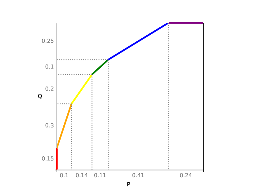
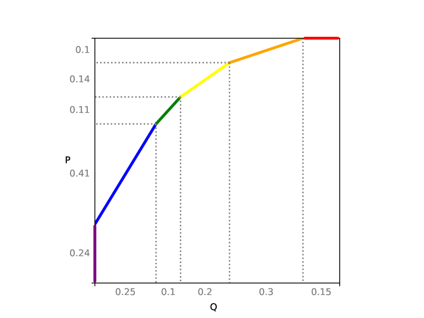
It is known that all divergences in $\mathcal{D}_{\textnormal{DPI}}$ between two distributions $P$ and $Q$ can be recovered from the power function between them. Recall that in this work, we focus on finite sample spaces; see Figure 1 for an example. It is known that power functions have a fractional knapsack interpretation [25].

Definition 34 (Power Function).

Suppose $P$ and $Q$ are distributions on the same sample space $\Omega$ .

$\blacksquare$

For a discrete sample space $\Omega$ , the power function $\mathsf{Pow}(P\|Q):[0,1]\rightarrow[0,1]$ can be defined in terms of the fractional knapsack problem.

Given a collection $\Omega$ of items, suppose $\omega\in\Omega$ has weight $P(\omega)$ and value $Q(\omega)$ . Then, given $x\in[0,1]$ , $\mathsf{Pow}(P\|Q)(x)$ is the maximum value attained with weight capacity constraint $x$ , where items may be taken fractionally.
$\blacksquare$

For a continuous sample space $\Omega$ , given $x\in[0,1]$ , $\mathsf{Pow}(P\|Q)(x)$ is the supremum of $Q(S)$ over measurable subsets $S\subseteq\Omega$ satisfying $P(S)=x$ .

Refer to caption — (a) $g=\mathsf{Pow}(P||Q)$ .

In the literature (see [16] for instance), the tradeoff function $\mathsf{T}(P\|Q):=1-\mathsf{Pow}(P\|Q)$ , which has essentially equivalent mathematical properties, has also been considered. However, power functions have the same notation interpretation as divergences in the sense that “smaller” means “closer” distributions. In fact, Vadhan and Zhang [38] defined an abstract concept of generalized probability distance (with the tradeoff function as the main example) such that the notation agrees with this interpretation. We recap some well-known properties of power functions.

Fact 35 (Valid power functions [16, Proposition 2.2]).

Suppose $g:[0,1]\rightarrow[0,1]$ is a function. Then, there exist distributions $X$ and $Y$ such that $\mathsf{Pow}(X\|Y)=g$ iff $g$ is continuous, concave and $g(x)\geq x$ for all $x\in[0,1]$ .

Partial Order on Power Functions.

We consider a partial order on power functions. Given such functions $g_{1}$ and $g_{2}$ , we denote $g_{1}\preceq g_{2}$ iff for all $x\in[0,1]$ , $g_{1}(x)\leq g_{2}(x)$ .

We next state formally how a divergence satisfying Definition 33 can be recovered from the power function.

Fact 36 (Recovering Divergence From Power Function [16, Proposition B.1]).

For any divergence $\mathsf{D}\in\mathcal{D}_{\textnormal{DPI}}$ , there exists a functional $\ell_{\mathsf{D}}:[0,1]^{[0,1]}\rightarrow\mathbb{R}$ such that for any distributions $P$ and $Q$ on the same sample space, $\mathsf{D}(P\|Q)=\ell_{\mathsf{D}}(\mathsf{Pow}(P\|Q))$ .

Moreover, if $g_{1}\preceq g_{2}$ , then $\ell_{\mathsf{D}}(g_{1})\leq\ell_{\mathsf{D}}(g_{2})$ .

The following is the main result of this section, which states that a locally maximin pair essentially solves the closest distribution refinement problem optimally in the most general sense.

Theorem 37 (Locally Maximin Pair Gives Minimal Power Function).

Suppose in a distribution instance $G$ , $\vec{\alpha}=(\alpha^{(0)},\alpha^{(1)})$ is a distribution refinement pair that is locally maximin and proportional response to each other. Then, the power function $g_{\mathchoice{\raisebox{0.0pt}{\leavevmode\resizebox{3.11111pt}{4.78333pt}{% \hbox{\raisebox{1.3611pt}{$\displaystyle{\dagger}$}}}}}{\raisebox{0.0pt}{% \leavevmode\resizebox{3.11111pt}{4.78333pt}{\hbox{\raisebox{1.3611pt}{$% \textstyle{\dagger}$}}}}}{\raisebox{0.0pt}{\leavevmode\resizebox{2.17778pt}{3.% 34833pt}{\hbox{\raisebox{0.95277pt}{$\scriptstyle{\dagger}$}}}}}{\raisebox{0.0% pt}{\leavevmode\resizebox{1.55556pt}{2.39166pt}{\hbox{\raisebox{0.68054pt}{$% \scriptscriptstyle{\dagger}$}}}}}}$ between any other distribution refinement pair of $G$ satisfies $\mathsf{Pow}(\alpha^{(0)}\|\alpha^{(1)})\preceq g_{\mathchoice{\raisebox{0.0pt% }{\leavevmode\resizebox{3.11111pt}{4.78333pt}{\hbox{\raisebox{1.3611pt}{$% \displaystyle{\dagger}$}}}}}{\raisebox{0.0pt}{\leavevmode\resizebox{3.11111pt}% {4.78333pt}{\hbox{\raisebox{1.3611pt}{$\textstyle{\dagger}$}}}}}{\raisebox{0.0% pt}{\leavevmode\resizebox{2.17778pt}{3.34833pt}{\hbox{\raisebox{0.95277pt}{$% \scriptstyle{\dagger}$}}}}}{\raisebox{0.0pt}{\leavevmode\resizebox{1.55556pt}{% 2.39166pt}{\hbox{\raisebox{0.68054pt}{$\scriptscriptstyle{\dagger}$}}}}}}$ . Consequently, any such locally maximin pair gives rise to the same power function, and we denote $\mathsf{Pow}^{*}(G)=\mathsf{Pow}(\alpha^{(0)}\|\alpha^{(1)})$ .

From Fact 36, this implies that $\vec{\alpha}$ is a universally closest refinement pair with respect to $\mathcal{D}_{\textnormal{DPI}}$ .

$\blacktriangleright$ Remark 38.

Observe that given any $\mathsf{D}\in\mathcal{D}_{\textnormal{DPI}}$ and any strictly increasing function $\phi:\mathbb{R}\rightarrow\mathbb{R}$ , we still have $\phi(\mathsf{D}(\cdot\|\cdot))\in\mathcal{D}_{\textnormal{DPI}}$ . Since any deviation from the correct answer can be arbitrarily magnified by $\phi$ , it is difficult to give any meaningful approximation guarantee on the value of a general divergence in $\mathcal{D}_{\textnormal{DPI}}$ .

We prove Theorem 37 by analyzing the relationship between hockey-stick divergence and power function, and extend the result from Theorem 32. Similar to convex functions, we also consider the notion of subgradient for power functions.

Definition 39 (Subgradient).

Suppose $g:[0,1]\rightarrow[0,1]$ is a power function and $x\in[0,1]$ . Then, the subgradient of $g$ at $x$ is defined as the collection $\partial g(x)$ of real numbers satisfying:

$\gamma\in\partial g(x)$ iff for all $y\in[0,1]$ , $g(x)+\gamma\cdot(y-x)\geq g(y)$ .

In other words, the line segment with slope $\gamma$ touching the curve $g$ at $x$ never goes below the curve.

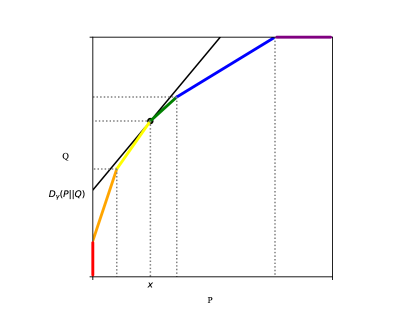
The following is a special case of Fact 36, and describes explicitly how a hockey-stick divergence is recovered from a power function. See Figure 2 for an illustration.

Fact 40 (Recovering Hockey-Stick Divergence From Power Function).

Suppose $P$ and $Q$ are distributions on the same sample space $\Omega$ , where $g=\mathsf{Pow}(P\|Q)$ is the power function between them. Then, for any $\gamma\geq 0$ , there exists $x\in[0,1]$ such that $\gamma\in\partial g(x)$ and $\mathsf{D}_{\gamma}(P\|Q)=g(x)-\gamma x$ .

In other words, one can find a line segment with slope $\gamma$ touching the curve $g$ and the $y$ -intercept of the line will give $\mathsf{D}_{\gamma}(P\|Q)$ .

Proof.

The result should be standard, but we include a short proof for completeness. One can imagine a line segment with slope $\gamma$ starting high above and gradually being lowered until touching the curve $g$ at some $x\in[0,1]$ . Observe that the line segment may touch the curve at more than 1 point, in which case we take $x$ to be the infimum.

We partition the sample space $\Omega$ into $S_{1}:=\{\omega\in\Omega:Q(\omega)>\gamma\cdot P(\omega)\}$ and $S_{2}:=\Omega\setminus S_{1}$ . Observe that $P(S_{1})=x$ and $g(x)=Q(S_{1})$ .

Then, it follows that $\mathsf{D}_{\gamma}(P\|Q)=Q(S_{1})-\gamma\cdot P(S_{1})=g(x)-\gamma x$ , as required. $\hfill\blacktriangleleft$

Proof of Theorem 37.

Suppose $g=\mathsf{Pow}(\alpha^{(0)}\|\alpha^{(1)})$ is the power function between the given locally maximin pair $\vec{\alpha}$ . For the sake of contradiction, suppose some other refinement pair $\vec{\alpha}_{\mathchoice{\raisebox{0.0pt}{\leavevmode\resizebox{3.11111pt}{4.% 78333pt}{\hbox{\raisebox{1.3611pt}{$\displaystyle{\dagger}$}}}}}{\raisebox{0.0% pt}{\leavevmode\resizebox{3.11111pt}{4.78333pt}{\hbox{\raisebox{1.3611pt}{$% \textstyle{\dagger}$}}}}}{\raisebox{0.0pt}{\leavevmode\resizebox{2.17778pt}{3.% 34833pt}{\hbox{\raisebox{0.95277pt}{$\scriptstyle{\dagger}$}}}}}{\raisebox{0.0% pt}{\leavevmode\resizebox{1.55556pt}{2.39166pt}{\hbox{\raisebox{0.68054pt}{$% \scriptscriptstyle{\dagger}$}}}}}}$ produces the power function $g_{\mathchoice{\raisebox{0.0pt}{\leavevmode\resizebox{3.11111pt}{4.78333pt}{% \hbox{\raisebox{1.3611pt}{$\displaystyle{\dagger}$}}}}}{\raisebox{0.0pt}{% \leavevmode\resizebox{3.11111pt}{4.78333pt}{\hbox{\raisebox{1.3611pt}{$% \textstyle{\dagger}$}}}}}{\raisebox{0.0pt}{\leavevmode\resizebox{2.17778pt}{3.% 34833pt}{\hbox{\raisebox{0.95277pt}{$\scriptstyle{\dagger}$}}}}}{\raisebox{0.0% pt}{\leavevmode\resizebox{1.55556pt}{2.39166pt}{\hbox{\raisebox{0.68054pt}{$% \scriptscriptstyle{\dagger}$}}}}}}$ such that for some $x\in[0,1]$ , $g(x)>g_{\mathchoice{\raisebox{0.0pt}{\leavevmode\resizebox{3.11111pt}{4.78333% pt}{\hbox{\raisebox{1.3611pt}{$\displaystyle{\dagger}$}}}}}{\raisebox{0.0pt}{% \leavevmode\resizebox{3.11111pt}{4.78333pt}{\hbox{\raisebox{1.3611pt}{$% \textstyle{\dagger}$}}}}}{\raisebox{0.0pt}{\leavevmode\resizebox{2.17778pt}{3.% 34833pt}{\hbox{\raisebox{0.95277pt}{$\scriptstyle{\dagger}$}}}}}{\raisebox{0.0% pt}{\leavevmode\resizebox{1.55556pt}{2.39166pt}{\hbox{\raisebox{0.68054pt}{$% \scriptscriptstyle{\dagger}$}}}}}}(x)$ .

Fix some $\gamma\in\partial g_{\mathchoice{\raisebox{0.0pt}{\leavevmode\resizebox{3.1111% 1pt}{4.78333pt}{\hbox{\raisebox{1.3611pt}{$\displaystyle{\dagger}$}}}}}{% \raisebox{0.0pt}{\leavevmode\resizebox{3.11111pt}{4.78333pt}{\hbox{\raisebox{1% .3611pt}{$\textstyle{\dagger}$}}}}}{\raisebox{0.0pt}{\leavevmode\resizebox{2.1% 7778pt}{3.34833pt}{\hbox{\raisebox{0.95277pt}{$\scriptstyle{\dagger}$}}}}}{% \raisebox{0.0pt}{\leavevmode\resizebox{1.55556pt}{2.39166pt}{\hbox{\raisebox{0% .68054pt}{$\scriptscriptstyle{\dagger}$}}}}}}(x)$ and consider the line segment $\ell_{\mathchoice{\raisebox{0.0pt}{\leavevmode\resizebox{3.11111pt}{4.78333pt}% {\hbox{\raisebox{1.3611pt}{$\displaystyle{\dagger}$}}}}}{\raisebox{0.0pt}{% \leavevmode\resizebox{3.11111pt}{4.78333pt}{\hbox{\raisebox{1.3611pt}{$% \textstyle{\dagger}$}}}}}{\raisebox{0.0pt}{\leavevmode\resizebox{2.17778pt}{3.% 34833pt}{\hbox{\raisebox{0.95277pt}{$\scriptstyle{\dagger}$}}}}}{\raisebox{0.0% pt}{\leavevmode\resizebox{1.55556pt}{2.39166pt}{\hbox{\raisebox{0.68054pt}{$% \scriptscriptstyle{\dagger}$}}}}}}$ with slope $\gamma$ touching curve $g_{\mathchoice{\raisebox{0.0pt}{\leavevmode\resizebox{3.11111pt}{4.78333pt}{% \hbox{\raisebox{1.3611pt}{$\displaystyle{\dagger}$}}}}}{\raisebox{0.0pt}{% \leavevmode\resizebox{3.11111pt}{4.78333pt}{\hbox{\raisebox{1.3611pt}{$% \textstyle{\dagger}$}}}}}{\raisebox{0.0pt}{\leavevmode\resizebox{2.17778pt}{3.% 34833pt}{\hbox{\raisebox{0.95277pt}{$\scriptstyle{\dagger}$}}}}}{\raisebox{0.0% pt}{\leavevmode\resizebox{1.55556pt}{2.39166pt}{\hbox{\raisebox{0.68054pt}{$% \scriptscriptstyle{\dagger}$}}}}}}$ at $x$ . By Fact 40, the hockey-stick divergence $\mathsf{D}_{\gamma}(\vec{\alpha}_{\mathchoice{\raisebox{0.0pt}{\leavevmode% \resizebox{3.11111pt}{4.78333pt}{\hbox{\raisebox{1.3611pt}{$\displaystyle{% \dagger}$}}}}}{\raisebox{0.0pt}{\leavevmode\resizebox{3.11111pt}{4.78333pt}{% \hbox{\raisebox{1.3611pt}{$\textstyle{\dagger}$}}}}}{\raisebox{0.0pt}{% \leavevmode\resizebox{2.17778pt}{3.34833pt}{\hbox{\raisebox{0.95277pt}{$% \scriptstyle{\dagger}$}}}}}{\raisebox{0.0pt}{\leavevmode\resizebox{1.55556pt}{% 2.39166pt}{\hbox{\raisebox{0.68054pt}{$\scriptscriptstyle{\dagger}$}}}}}})$ is the $y$ -intercept of $\ell_{\mathchoice{\raisebox{0.0pt}{\leavevmode\resizebox{3.11111pt}{4.78333pt}% {\hbox{\raisebox{1.3611pt}{$\displaystyle{\dagger}$}}}}}{\raisebox{0.0pt}{% \leavevmode\resizebox{3.11111pt}{4.78333pt}{\hbox{\raisebox{1.3611pt}{$% \textstyle{\dagger}$}}}}}{\raisebox{0.0pt}{\leavevmode\resizebox{2.17778pt}{3.% 34833pt}{\hbox{\raisebox{0.95277pt}{$\scriptstyle{\dagger}$}}}}}{\raisebox{0.0% pt}{\leavevmode\resizebox{1.55556pt}{2.39166pt}{\hbox{\raisebox{0.68054pt}{$% \scriptscriptstyle{\dagger}$}}}}}}$ .

However, since $g(x)>g_{\mathchoice{\raisebox{0.0pt}{\leavevmode\resizebox{3.11111pt}{4.78333% pt}{\hbox{\raisebox{1.3611pt}{$\displaystyle{\dagger}$}}}}}{\raisebox{0.0pt}{% \leavevmode\resizebox{3.11111pt}{4.78333pt}{\hbox{\raisebox{1.3611pt}{$% \textstyle{\dagger}$}}}}}{\raisebox{0.0pt}{\leavevmode\resizebox{2.17778pt}{3.% 34833pt}{\hbox{\raisebox{0.95277pt}{$\scriptstyle{\dagger}$}}}}}{\raisebox{0.0% pt}{\leavevmode\resizebox{1.55556pt}{2.39166pt}{\hbox{\raisebox{0.68054pt}{$% \scriptscriptstyle{\dagger}$}}}}}}(x)$ , to find a line segment with slope $\gamma$ touching curve $g$ , we must move $\ell_{\mathchoice{\raisebox{0.0pt}{\leavevmode\resizebox{3.11111pt}{4.78333pt}% {\hbox{\raisebox{1.3611pt}{$\displaystyle{\dagger}$}}}}}{\raisebox{0.0pt}{% \leavevmode\resizebox{3.11111pt}{4.78333pt}{\hbox{\raisebox{1.3611pt}{$% \textstyle{\dagger}$}}}}}{\raisebox{0.0pt}{\leavevmode\resizebox{2.17778pt}{3.% 34833pt}{\hbox{\raisebox{0.95277pt}{$\scriptstyle{\dagger}$}}}}}{\raisebox{0.0% pt}{\leavevmode\resizebox{1.55556pt}{2.39166pt}{\hbox{\raisebox{0.68054pt}{$% \scriptscriptstyle{\dagger}$}}}}}}$ strictly upwards. This implies that $\mathsf{D}_{\gamma}(\vec{\alpha})>\mathsf{D}_{\gamma}(\vec{\alpha}_{% \mathchoice{\raisebox{0.0pt}{\leavevmode\resizebox{3.11111pt}{4.78333pt}{\hbox% {\raisebox{1.3611pt}{$\displaystyle{\dagger}$}}}}}{\raisebox{0.0pt}{% \leavevmode\resizebox{3.11111pt}{4.78333pt}{\hbox{\raisebox{1.3611pt}{$% \textstyle{\dagger}$}}}}}{\raisebox{0.0pt}{\leavevmode\resizebox{2.17778pt}{3.% 34833pt}{\hbox{\raisebox{0.95277pt}{$\scriptstyle{\dagger}$}}}}}{\raisebox{0.0% pt}{\leavevmode\resizebox{1.55556pt}{2.39166pt}{\hbox{\raisebox{0.68054pt}{$% \scriptscriptstyle{\dagger}$}}}}}})$ , contradicting Theorem 32 which states that $\vec{\alpha}$ is universally closest with respect to $\mathcal{D}_{\textnormal{HS}}$ . $\hfill\blacktriangleleft$

References

[1] Albert Angel, Nikos Sarkas, Nick Koudas, and Divesh Srivastava. Dense subgraph maintenance under streaming edge weight updates for real-time story identification. Proceedings of the VLDB Endowment, 5(6):574–585, 2012. doi:10.14778/2168651.2168658.
[2] Kenneth J Arrow and Gerard Debreu. Existence of an equilibrium for a competitive economy. Econometrica: Journal of the Econometric Society, pages 265–290, 1954.
[3] Oana Denisa Balalau, Francesco Bonchi, T.-H. Hubert Chan, Francesco Gullo, and Mauro Sozio. Finding subgraphs with maximum total density and limited overlap. In WSDM, pages 379–388. ACM, 2015. doi:10.1145/2684822.2685298.
[4] Nikhil Bansal and Ilan Reuven Cohen. Contention resolution, matrix scaling and fair allocation. In WAOA, volume 12982 of Lecture Notes in Computer Science, pages 252–274. Springer, 2021. doi:10.1007/978-3-030-92702-8_16.
[5] Amir Beck and Marc Teboulle. A fast iterative shrinkage-thresholding algorithm for linear inverse problems. SIAM journal on imaging sciences, 2(1):183–202, 2009. doi:10.1137/080716542.
[6] Roger E Behrend. Fractional perfect b-matching polytopes i: General theory. Linear Algebra and its Applications, 439(12):3822–3858, 2013.
[7] Aaron Bernstein, Jacob Holm, and Eva Rotenberg. Online bipartite matching with amortized O(log ${}^{\mbox{2}}$ n) replacements. J. ACM, 66(5):37:1–37:23, 2019. doi:10.1145/3344999.
[8] Benjamin Birnbaum, Nikhil R Devanur, and Lin Xiao. Distributed algorithms via gradient descent for fisher markets. In Proceedings of the 12th ACM conference on Electronic commerce, pages 127–136, 2011. doi:10.1145/1993574.1993594.
[9] Richard A Brualdi. Combinatorial matrix classes, volume 13. Cambridge University Press, 2006.
[10] Niv Buchbinder, Anupam Gupta, Daniel Hathcock, Anna R. Karlin, and Sherry Sarkar. Maintaining matroid intersections online. In SODA, pages 4283–4304. SIAM, 2024. doi:10.1137/1.9781611977912.149.
[11] T.-H. Hubert Chan, Anand Louis, Zhihao Gavin Tang, and Chenzi Zhang. Spectral properties of hypergraph laplacian and approximation algorithms. J. ACM, 65(3):15:1–15:48, 2018. doi:10.1145/3178123.
[12] T.-H. Hubert Chan and Quan Xue. Symmetric splendor: Unraveling universally closest refinements and fisher market equilibrium through density-friendly decomposition. CoRR, abs/2406.17964, 2024. doi:10.48550/arXiv.2406.17964.
[13] Moses Charikar. Greedy approximation algorithms for finding dense components in a graph. In Klaus Jansen and Samir Khuller, editors, Approximation Algorithms for Combinatorial Optimization, pages 84–95, Berlin, Heidelberg, 2000. Springer Berlin Heidelberg. doi:10.1007/3-540-44436-X_10.
[14] Li Chen, Rasmus Kyng, Yang P. Liu, Richard Peng, Maximilian Probst Gutenberg, and Sushant Sachdeva. Maximum flow and minimum-cost flow in almost-linear time. In FOCS, pages 612–623. IEEE, 2022. doi:10.1109/FOCS54457.2022.00064.
[15] Maximilien Danisch, T.-H. Hubert Chan, and Mauro Sozio. Large scale density-friendly graph decomposition via convex programming. In WWW, pages 233–242. ACM, 2017. doi:10.1145/3038912.3052619.
[16] Jinshuo Dong, Aaron Roth, and Weijie J Su. Gaussian differential privacy. Journal of the Royal Statistical Society Series B: Statistical Methodology, 84(1):3–37, 2022.
[17] Cynthia Dwork. Differential privacy. In ICALP (2), volume 4052 of Lecture Notes in Computer Science, pages 1–12. Springer, 2006. doi:10.1007/11787006_1.
[18] Irving Fisher. Mathematical investigations in the theory of value and prices, 1892.
[19] Satoru Fujishige. Lexicographically optimal base of a polymatroid with respect to a weight vector. Mathematics of Operations Research, 5(2):186–196, 1980. doi:10.1287/MOOR.5.2.186.
[20] Ashish Goel, Michael Kapralov, and Sanjeev Khanna. On the communication and streaming complexity of maximum bipartite matching. In SODA, pages 468–485. SIAM, 2012. doi:10.1137/1.9781611973099.41.
[21] Andrew V Goldberg. Finding a maximum density subgraph, 1984.
[22] Elfarouk Harb, Kent Quanrud, and Chandra Chekuri. Faster and scalable algorithms for densest subgraph and decomposition. Advances in Neural Information Processing Systems, 35:26966–26979, 2022.
[23] Elfarouk Harb, Kent Quanrud, and Chandra Chekuri. Convergence to lexicographically optimal base in a (contra)polymatroid and applications to densest subgraph and tree packing. In ESA, volume 274 of LIPIcs, pages 56:1–56:17. Schloss Dagstuhl – Leibniz-Zentrum für Informatik, 2023. doi:10.4230/LIPICS.ESA.2023.56.
[24] Kamal Jain and Vijay V. Vazirani. Eisenberg-gale markets: Algorithms and game-theoretic properties. Games Econ. Behav., 70(1):84–106, 2010. doi:10.1016/J.GEB.2008.11.011.
[25] Joseph B Kadane. Discrete search and the neyman-pearson lemma. Journal of Mathematical Analysis and Applications, 22(1):156–171, 1968.
[26] Samir Khuller and Barna Saha. On finding dense subgraphs. In International colloquium on automata, languages, and programming, pages 597–608. Springer, 2009. doi:10.1007/978-3-642-02927-1_50.
[27] Bernhard H. Korte. Combinatorial optimization: theory and algorithms. Springer, 2000.
[28] Euiwoong Lee and Sahil Singla. Maximum matching in the online batch-arrival model. ACM Trans. Algorithms, 16(4):49:1–49:31, 2020. doi:10.1145/3399676.
[29] Xiangfeng Li, Shenghua Liu, Zifeng Li, Xiaotian Han, Chuan Shi, Bryan Hooi, He Huang, and Xueqi Cheng. Flowscope: Spotting money laundering based on graphs. In Proceedings of the AAAI conference on artificial intelligence, volume 34(04), pages 4731–4738, 2020. doi:10.1609/AAAI.V34I04.5906.
[30] Chenhao Ma, Yixiang Fang, Reynold Cheng, Laks VS Lakshmanan, Wenjie Zhang, and Xuemin Lin. Efficient algorithms for densest subgraph discovery on large directed graphs. In Proceedings of the 2020 ACM SIGMOD International Conference on Management of Data, pages 1051–1066, 2020. doi:10.1145/3318464.3389697.
[31] Ilya Mironov. Rényi differential privacy. In CSF, pages 263–275. IEEE Computer Society, 2017. doi:10.1109/CSF.2017.11.
[32] Rajeev Motwani, Rina Panigrahy, and Ying Xu. Fractional matching via balls-and-bins. In APPROX-RANDOM, volume 4110 of Lecture Notes in Computer Science, pages 487–498. Springer, 2006. doi:10.1007/11830924_44.
[33] Yurii Nesterov. A method for solving the convex programming problem with convergence rate $o(1/k^{2})$ . Proceedings of the USSR Academy of Sciences, 269:543–547, 1983. URL: https://api.semanticscholar.org/CorpusID:145918791.
[34] Alexander Schrijver et al. Combinatorial optimization: polyhedra and efficiency, volume 24(2). Springer, 2003.
[35] Kijung Shin, Tina Eliassi-Rad, and Christos Faloutsos. Corescope: Graph mining using k-core analysis – Patterns, anomalies and algorithms. In 2016 IEEE 16th international conference on data mining (ICDM), pages 469–478. IEEE, 2016. doi:10.1109/ICDM.2016.0058.
[36] Nikolaj Tatti. Density-friendly graph decomposition. ACM Transactions on Knowledge Discovery from Data (TKDD), 13(5):1–29, 2019. doi:10.1145/3344210.
[37] Nikolaj Tatti and Aristides Gionis. Density-friendly graph decomposition. In Proceedings of the 24th International Conference on World Wide Web, pages 1089–1099, 2015. doi:10.1145/2736277.2741119.
[38] Salil P. Vadhan and Wanrong Zhang. Concurrent composition theorems for differential privacy. In STOC, pages 507–519. ACM, 2023. doi:10.1145/3564246.3585241.
[39] Fang Wu and Li Zhang. Proportional response dynamics leads to market equilibrium. In Proceedings of the thirty-ninth annual ACM symposium on Theory of computing, pages 354–363, 2007. doi:10.1145/1250790.1250844.
[40] Li Zhang. Proportional response dynamics in the fisher market. In ICALP (2), volume 5556 of Lecture Notes in Computer Science, pages 583–594. Springer, 2009. doi:10.1007/978-3-642-02930-1_48.
[41] Mingxun Zhou, Elaine Shi, T.-H. Hubert Chan, and Shir Maimon. A theory of composition for differential obliviousness. In EUROCRYPT (3), volume 14006 of Lecture Notes in Computer Science, pages 3–34. Springer, 2023. doi:10.1007/978-3-031-30620-4_1.
[42] Mingxun Zhou, Mengshi Zhao, T.-H. Hubert Chan, and Elaine Shi. Advanced composition theorems for differential obliviousness. In ITCS, volume 287 of LIPIcs, pages 103:1–103:24. Schloss Dagstuhl – Leibniz-Zentrum für Informatik, 2024. doi:10.4230/LIPICS.ITCS.2024.103.

[bib.bib1] [1] Albert Angel, Nikos Sarkas, Nick Koudas, and Divesh Srivastava. Dense subgraph maintenance under streaming edge weight updates for real-time story identification. Proceedings of the VLDB Endowment, 5(6):574–585, 2012. doi:10.14778/2168651.2168658.

[bib.bib2] [2] Kenneth J Arrow and Gerard Debreu. Existence of an equilibrium for a competitive economy. Econometrica: Journal of the Econometric Society, pages 265–290, 1954.

[bib.bib3] [3] Oana Denisa Balalau, Francesco Bonchi, T.-H. Hubert Chan, Francesco Gullo, and Mauro Sozio. Finding subgraphs with maximum total density and limited overlap. In WSDM, pages 379–388. ACM, 2015. doi:10.1145/2684822.2685298.

[bib.bib4] [4] Nikhil Bansal and Ilan Reuven Cohen. Contention resolution, matrix scaling and fair allocation. In WAOA, volume 12982 of Lecture Notes in Computer Science, pages 252–274. Springer, 2021. doi:10.1007/978-3-030-92702-8_16.

[bib.bib5] [5] Amir Beck and Marc Teboulle. A fast iterative shrinkage-thresholding algorithm for linear inverse problems. SIAM journal on imaging sciences, 2(1):183–202, 2009. doi:10.1137/080716542.

[bib.bib6] [6] Roger E Behrend. Fractional perfect b-matching polytopes i: General theory. Linear Algebra and its Applications, 439(12):3822–3858, 2013.

[bib.bib7] [7] Aaron Bernstein, Jacob Holm, and Eva Rotenberg. Online bipartite matching with amortized O(log ${}^{\mbox{2}}$ n) replacements. J. ACM, 66(5):37:1–37:23, 2019. doi:10.1145/3344999.

[bib.bib8] [8] Benjamin Birnbaum, Nikhil R Devanur, and Lin Xiao. Distributed algorithms via gradient descent for fisher markets. In Proceedings of the 12th ACM conference on Electronic commerce, pages 127–136, 2011. doi:10.1145/1993574.1993594.

[bib.bib9] [9] Richard A Brualdi. Combinatorial matrix classes, volume 13. Cambridge University Press, 2006.

[bib.bib10] [10] Niv Buchbinder, Anupam Gupta, Daniel Hathcock, Anna R. Karlin, and Sherry Sarkar. Maintaining matroid intersections online. In SODA, pages 4283–4304. SIAM, 2024. doi:10.1137/1.9781611977912.149.

[bib.bib11] [11] T.-H. Hubert Chan, Anand Louis, Zhihao Gavin Tang, and Chenzi Zhang. Spectral properties of hypergraph laplacian and approximation algorithms. J. ACM, 65(3):15:1–15:48, 2018. doi:10.1145/3178123.

[bib.bib12] [12] T.-H. Hubert Chan and Quan Xue. Symmetric splendor: Unraveling universally closest refinements and fisher market equilibrium through density-friendly decomposition. CoRR, abs/2406.17964, 2024. doi:10.48550/arXiv.2406.17964.

[bib.bib13] [13] Moses Charikar. Greedy approximation algorithms for finding dense components in a graph. In Klaus Jansen and Samir Khuller, editors, Approximation Algorithms for Combinatorial Optimization, pages 84–95, Berlin, Heidelberg, 2000. Springer Berlin Heidelberg. doi:10.1007/3-540-44436-X_10.

[bib.bib14] [14] Li Chen, Rasmus Kyng, Yang P. Liu, Richard Peng, Maximilian Probst Gutenberg, and Sushant Sachdeva. Maximum flow and minimum-cost flow in almost-linear time. In FOCS, pages 612–623. IEEE, 2022. doi:10.1109/FOCS54457.2022.00064.

[bib.bib15] [15] Maximilien Danisch, T.-H. Hubert Chan, and Mauro Sozio. Large scale density-friendly graph decomposition via convex programming. In WWW, pages 233–242. ACM, 2017. doi:10.1145/3038912.3052619.

[bib.bib16] [16] Jinshuo Dong, Aaron Roth, and Weijie J Su. Gaussian differential privacy. Journal of the Royal Statistical Society Series B: Statistical Methodology, 84(1):3–37, 2022.

[bib.bib17] [17] Cynthia Dwork. Differential privacy. In ICALP (2), volume 4052 of Lecture Notes in Computer Science, pages 1–12. Springer, 2006. doi:10.1007/11787006_1.

[bib.bib18] [18] Irving Fisher. Mathematical investigations in the theory of value and prices, 1892.

[bib.bib19] [19] Satoru Fujishige. Lexicographically optimal base of a polymatroid with respect to a weight vector. Mathematics of Operations Research, 5(2):186–196, 1980. doi:10.1287/MOOR.5.2.186.

[bib.bib20] [20] Ashish Goel, Michael Kapralov, and Sanjeev Khanna. On the communication and streaming complexity of maximum bipartite matching. In SODA, pages 468–485. SIAM, 2012. doi:10.1137/1.9781611973099.41.

[bib.bib21] [21] Andrew V Goldberg. Finding a maximum density subgraph, 1984.

[bib.bib22] [22] Elfarouk Harb, Kent Quanrud, and Chandra Chekuri. Faster and scalable algorithms for densest subgraph and decomposition. Advances in Neural Information Processing Systems, 35:26966–26979, 2022.

[bib.bib23] [23] Elfarouk Harb, Kent Quanrud, and Chandra Chekuri. Convergence to lexicographically optimal base in a (contra)polymatroid and applications to densest subgraph and tree packing. In ESA, volume 274 of LIPIcs, pages 56:1–56:17. Schloss Dagstuhl – Leibniz-Zentrum für Informatik, 2023. doi:10.4230/LIPICS.ESA.2023.56.

[bib.bib24] [24] Kamal Jain and Vijay V. Vazirani. Eisenberg-gale markets: Algorithms and game-theoretic properties. Games Econ. Behav., 70(1):84–106, 2010. doi:10.1016/J.GEB.2008.11.011.

[bib.bib25] [25] Joseph B Kadane. Discrete search and the neyman-pearson lemma. Journal of Mathematical Analysis and Applications, 22(1):156–171, 1968.

[bib.bib26] [26] Samir Khuller and Barna Saha. On finding dense subgraphs. In International colloquium on automata, languages, and programming, pages 597–608. Springer, 2009. doi:10.1007/978-3-642-02927-1_50.

[bib.bib27] [27] Bernhard H. Korte. Combinatorial optimization: theory and algorithms. Springer, 2000.

[bib.bib28] [28] Euiwoong Lee and Sahil Singla. Maximum matching in the online batch-arrival model. ACM Trans. Algorithms, 16(4):49:1–49:31, 2020. doi:10.1145/3399676.

[bib.bib29] [29] Xiangfeng Li, Shenghua Liu, Zifeng Li, Xiaotian Han, Chuan Shi, Bryan Hooi, He Huang, and Xueqi Cheng. Flowscope: Spotting money laundering based on graphs. In Proceedings of the AAAI conference on artificial intelligence, volume 34(04), pages 4731–4738, 2020. doi:10.1609/AAAI.V34I04.5906.

[bib.bib30] [30] Chenhao Ma, Yixiang Fang, Reynold Cheng, Laks VS Lakshmanan, Wenjie Zhang, and Xuemin Lin. Efficient algorithms for densest subgraph discovery on large directed graphs. In Proceedings of the 2020 ACM SIGMOD International Conference on Management of Data, pages 1051–1066, 2020. doi:10.1145/3318464.3389697.

[bib.bib31] [31] Ilya Mironov. Rényi differential privacy. In CSF, pages 263–275. IEEE Computer Society, 2017. doi:10.1109/CSF.2017.11.

[bib.bib32] [32] Rajeev Motwani, Rina Panigrahy, and Ying Xu. Fractional matching via balls-and-bins. In APPROX-RANDOM, volume 4110 of Lecture Notes in Computer Science, pages 487–498. Springer, 2006. doi:10.1007/11830924_44.

[bib.bib33] [33] Yurii Nesterov. A method for solving the convex programming problem with convergence rate $o(1/k^{2})$ . Proceedings of the USSR Academy of Sciences, 269:543–547, 1983. URL: https://api.semanticscholar.org/CorpusID:145918791.

[bib.bib34] [34] Alexander Schrijver et al. Combinatorial optimization: polyhedra and efficiency, volume 24(2). Springer, 2003.

[bib.bib35] [35] Kijung Shin, Tina Eliassi-Rad, and Christos Faloutsos. Corescope: Graph mining using k-core analysis – Patterns, anomalies and algorithms. In 2016 IEEE 16th international conference on data mining (ICDM), pages 469–478. IEEE, 2016. doi:10.1109/ICDM.2016.0058.

[bib.bib36] [36] Nikolaj Tatti. Density-friendly graph decomposition. ACM Transactions on Knowledge Discovery from Data (TKDD), 13(5):1–29, 2019. doi:10.1145/3344210.

[bib.bib37] [37] Nikolaj Tatti and Aristides Gionis. Density-friendly graph decomposition. In Proceedings of the 24th International Conference on World Wide Web, pages 1089–1099, 2015. doi:10.1145/2736277.2741119.

[bib.bib38] [38] Salil P. Vadhan and Wanrong Zhang. Concurrent composition theorems for differential privacy. In STOC, pages 507–519. ACM, 2023. doi:10.1145/3564246.3585241.

[bib.bib39] [39] Fang Wu and Li Zhang. Proportional response dynamics leads to market equilibrium. In Proceedings of the thirty-ninth annual ACM symposium on Theory of computing, pages 354–363, 2007. doi:10.1145/1250790.1250844.

[bib.bib40] [40] Li Zhang. Proportional response dynamics in the fisher market. In ICALP (2), volume 5556 of Lecture Notes in Computer Science, pages 583–594. Springer, 2009. doi:10.1007/978-3-642-02930-1_48.

[bib.bib41] [41] Mingxun Zhou, Elaine Shi, T.-H. Hubert Chan, and Shir Maimon. A theory of composition for differential obliviousness. In EUROCRYPT (3), volume 14006 of Lecture Notes in Computer Science, pages 3–34. Springer, 2023. doi:10.1007/978-3-031-30620-4_1.

[bib.bib42] [42] Mingxun Zhou, Mengshi Zhao, T.-H. Hubert Chan, and Elaine Shi. Advanced composition theorems for differential obliviousness. In ITCS, volume 287 of LIPIcs, pages 103:1–103:24. Schloss Dagstuhl – Leibniz-Zentrum für Informatik, 2024. doi:10.4230/LIPICS.ITCS.2024.103.

Unraveling Universally Closest Refinements via Symmetric Density Decomposition and Fisher Market Equilibrium

Abstract

Keywords and phrases:

Funding:

Copyright and License:

2012 ACM Subject Classification:

Related Version:

DOI:

Event:

Editors:

Series and Publisher:

1 Introduction

Definition 1 (Closest Distribution Refinement Problem).

Theorem 2 (Universally Closest Refinement Pair).

1.1 Our Technical Contributions and Approaches

Goal 3 (High-Level Goal).

1.1.1 Hypergraph Density Decomposition

Densest Subset Problem.

Density Decomposition.

Connection with the Local Maximin Condition.

Symmetry of Density Decomposition.

Approximation Notions.

1.1.2 Unraveling Universally Closest Distribution Refinements via Symmetric Density Decomposition

Restricted Class of Divergence.

Universal Refinement Matching Problem.

Theorem 4 (Universal Maximum Refinement Matching).

Extension to General Case.

Approximation Results.

1.1.3 Achieving Multiplicative Error via Proportional Response in Fisher Markets

Market Interpretation.

Alternative Characterization.

1.2 Motivation and Application for Universally Closest Distribution Refinements

A Quick Introduction to Differential Privacy/Obliviousness.

Composition of Differentially Oblivious Mechanisms.

Fact 5 (Lemma B.1 in [42]).

1.3 Related Work

Density Decomposition.

Symmetric Nature of Density Decomposition.

Connection between Density Decomposition and Fisher Market Equilibrium.

Distributed Iterative Approximation Algorithms.

Density Decomposition.

1.4 Potential Impacts and Paper Organization

2 Preliminaries

Definition 6 (Input Instance).

▶ Remark 7.

Definition 8 (Allocation Refinement and Payload).

Definition 9 (Proportional Response).

Definition 10 (Local Maximin Condition).

▶ Remark 11.

Definition 12 (Notions of Error).

3 Folklore: Symmetric Density Decomposition

Notation: Ground and Auxiliary Sets.

Definition 13 (Densest Subset).

Fact 14.

Definition 15 (Sub-Instance).

Definition 16 (Density Decomposition with Ground Set).

▶ Remark 17 (Isolated Vertices).

Fact 18 (Local Maximin Condition Gives Density Decomposition).

Symmetry in Density Decomposition.

Lemma 19 (Proportional Response to Locally Maximin Refinement).

Theorem 20 (Folklore: Symmetry of Density Decomposition).

4 Universal Refinement Matching Problem

Definition 21 (Vertex-Constrained Matching Instance).

LP Interpretation.

Definition 22 (Fractional Matching Induced by Refinement Pair).

▶ Remark 23.

Definition 24 (Universal Refinement Pair for Matching).

Intuition for Universal Refinement Pair.

Lemma 25 (Local Maximin Achieves Universal for Matching).

Proof.

5 Universally Closest Distribution Refinements Problem

Distribution Instance.

Divergence Notion.

Definition 26 (Closest Refinement Pair).

▶ Remark 27.

Definition 28 (Universally Closest Refinement Pair).

5.1 Class of Hockey-Stick Divergences

Definition 29 (Hockey-Stick Divergence).

▶ Remark 30.

Lemma 31 (Hockey-Stick Divergence and Matching).

$\blacktriangleright$ Remark 7.

$\blacktriangleright$ Remark 11.

$\blacktriangleright$ Remark 17 (Isolated Vertices).

$\blacktriangleright$ Remark 23.

$\blacktriangleright$ Remark 27.

$\blacktriangleright$ Remark 30.

Theorem 32 (Locally Maximin Pair is Closest for $\mathcal{D}_{\textnormal{HS}}$ ).

$\blacktriangleright$ Remark 38.