Derandomized Squaring: An Analytical Insight into Its True Behavior

Abstract
The notion of the derandomized square of two graphs, denoted as , was introduced by Rozenman and Vadhan as they rederived Reingold’s Theorem, . This pseudorandom primitive, closely related to the Zig-Zag product, plays a crucial role in recent advancements on space-bounded derandomization. For this and other reasons, understanding the spectral expansion becomes paramount. Rozenman and Vadhan derived an upper bound for in terms of the spectral expansions of the individual graphs, and . They also proved their bound is optimal if the only information incorporated to the bound is the spectral expansion of the two graphs.
The objective of this work is to gain deeper insights into the behavior of derandomized squaring by taking into account the entire spectrum of , where we focus on a vertex-transitive -regular . Utilizing deep results from analytic combinatorics, we establish a lower bound on that applies universally to all graphs . Our work reveals that the bound is the minimum value of the function
in the domain , where is the characteristic polynomial of the -vertex graph . This bound lies far below the known upper bound for for most reasonable choices for . Empirical evidence suggests that our lower bound is optimal. We support the tightness of our lower bound by showing that the bound is tight for a class of graphs which exhibit local behavior similar to a derandomized squaring operation with . To this end, we make use of finite free probability theory.
In our second result, we resolve an open question posed by Cohen and Maor (STOC 2023) and establish a lower bound for the spectral expansion of rotating expanders. These graphs are constructed by taking a random walk with vertex permutations occurring after each step. We prove that Cohen and Maor’s construction is essentially optimal. Unlike our results on derandomized squaring, the proof in this instance relies solely on combinatorial methods. The key insight lies in establishing a connection between random walks on graph products and the Fuss-Catalan numbers.
Keywords and phrases:
Derandomized Squaring, Spectral Graph Theory, Analytic CombinatoricsFunding:
Gil Cohen: Supported by ERC starting grant 949499 and by the Israel ScienceFoundation grant 1569/18.
grant 1569/18.
grant 1569/18.
Copyright and License:
2012 ACM Subject Classification:
Mathematics of computing Spectra of graphsEditors:
Raghu MekaSeries and Publisher:
1 Introduction
Expander graphs have played a crucial role in essentially all areas within theoretical computer science as well as in coding theory, and cryptography, among others. Their utility stems to a large extent from the ability to interpret expansion from various perspectives, be it combinatorial, probabilistic, or linear algebraic. This multifaceted understanding offers a unique advantage: it enables the otherwise challenging inference of combinatorial attributes of graphs by examining the spectral properties of related operators.
We briefly recall the notion of spectral expansion. Let be an undirected -regular graph on vertices with adjacency matrix . Since is undirected, is symmetric and so its spectrum is real-valued. We denote the eigenvalues of by . The spectral expansion of , denoted as , is given by . We further denote the normalized spectral expansion of by . We alternate between the two variants–the normalized and the unnormalized–depending on context.
An expander is a graph with a normalized spectral expansion that is bounded away from 111To be more precise, it is common to consider a family of graphs in this context. However, we will exclude this technical detail from our discussion for simplicity.. However, for a typical application of expander graphs one “pays” a cost that increases with the degree and has an “error” that vanishes as . This raises the question of what is the lowest possible value of attainable by -regular graphs. From the Alon-Boppana bound [30], which is usually stated in terms of , it follows that for every there are only finitely many -regular graphs with . A -regular graph satisfying is called a Ramanujan graph. Over the past several decades, Ramanujan graphs have been a focal point of research. The constructions of Ramanujan graphs and their variants lean on profound number theoretic results [19, 24, 27] (see also [18]), or is rooted in deep analytical methods and on the accompanied technique of polynomial interlacing [20, 23, 22, 13, 16].
In their highly influential paper [34], Reingold, Vadhan, and Wigderson introduced the Zig-Zag product which enabled them to obtain a combinatorial construction of expander graphs by elementary means. While the expanders that were constructed were not quite close to Ramanujan, the fact that the construction is combinatorial and highly flexible made the Zig-Zag product extremely useful. Indeed, no long after, Reingold [33] based his breakthrough result, , on the Zig-Zag product, not for constructing expanders per se but for the purpose of “transforming” a given graph to an expander while maintaining its connected components structure. In a subsequent work, Ben-Aroya and Ta-Shma [5] put forth an improved variant of the Zig-Zag product, dubbed the wide-replacement product, that enabled the combinatorial construction of graphs that come quite close to Ramanujan. That variant was key in a recent breakthrough by Ta-Shma who constructed near-optimal small-bias sets [36]. Several other expander construction paradigms have been put forth in the literature, e.g., [6, 26]. We refer the reader to the excellent survey by Hoory, Linial, and Wigderson [17] for a comprehensive exposition on expander graphs.
1.1 Derandomized squaring
Not long after the work of Reingold [33], Rozenman and Vadhan [35] introduced a close sibling to the Zig-Zag product, dubbed derandomized squaring, which we describe soon. This operation can be “cleaner” than the Zig-Zag product in some settings, in particular for their rederivation of Reingold’s result, though the two operations are tightly connected. In the past few years, derandomized squaring has gained significant traction in the space-bounded derandomization literature (see, e.g., [28, 1, 2, 11]) mostly since it facilitated the adaptation of ideas from the realm of fast Laplacian solvers into the domain of space-bounded derandomization. For these reasons, in this paper we focus on the operation of derandomized squaring though we are confident that our techniques can be extended to other operations such as the Zig-Zag product and the wide-replacement product.
Squaring a graph is an easy way of improving its normalized spectral expansion. The square of a graph , denoted as , is the graph on the same vertex set that has an edge between a pair of vertices for every length- path in between the vertices. Clearly, if is the adjacency matrix of then is the adjacency matrix of . Hence, . However, if is -regular, is a -regular graph. As a result, the degree growth associated with squaring the graph often surpasses the advantages gained from reducing the normalized spectral expansion. The purpose of derandomized squaring is to obtain a comparable improvement to the normalized spectral expansion without blowing up the degree by a quadratic factor.
From the view point of a vertex of , in the graph , the neighbors of are all connected to each other. That is, is obtained by adding copies of the complete graph with self-loops, one copy for each vertex , where the complete graph associated with is placed on the neighbors of . Let be a graph on vertices, where we focus on the case in which is vertex-transitive, and denote the degree of a vertex in by . The derandomized square of and , denoted as , is defined by replacing each such copy of the complete graph with a copy of . Note that is a -regular graph where . Formally, the derandomized squaring, like the Zig-Zag product, requires working with edge-labeled graphs, but we sidestep this technicality. For the reader that is familiar with these intricacies, we remark that, for simplicity, in this extended abstract we circumvent labeling issues by assuming that is given as the union of perfect matchings, though this condition can be relaxed.
Given that an expander approximates the complete graph, one is correct to expect that the derandomized square approximates for every graph . Rozenman and Vadhan formalized this intuition with regards to the normalized spectral expansion by establishing the bound
| (1.1) |
How tight is this bound? This is a somewhat subtle question. Rozenman and Vadhan proved that the bound is tight as a function of and , however, it is certainly conceivable that a superior bound might be achieved if one incorporates more information about the graphs beyond just their spectral expansions into the bound. In particular, if we fix and consider the mapping which maps every -regular graph to , then it is interesting to ask how strong a bound can be obtained on this mapping as a function of the entire spectrum of .
Given the significance of the derandomized squaring operation, and the related Zig Zag product as well as the wide-replacement product, a substantial improvement to the bound could profoundly impact our understanding on several fundamental problems, including in space-bounded derandomization and in coding theory. For example, in the context of space-bounded derandomization such a result may reduce the seed length of PRGs or weighted PRGs (see [9, 10, 11] and references therein). Such a result may also lead to a better construction of small-bias sets in which the wide-replacement product is used for bias-reduction. Therefore, gaining a thorough understanding of derandomized squaring is highly motivated from the theoretical computer science standpoint.
1.2 Two case studies
Before presenting our results, which we view as a first step towards the above goal, we wish to highlight the gap between the Rozenman-Vadhan bound, as given in Equation 1.1, and the “true” behavior of the derandomized squaring operation. We do so by considering two case studies, starting with , the complete -regular bipartite graph on vertices.
1.2.1 Derandomized squaring with the complete regular bipartite graph
Since is bipartite, , and so the bound given by Equation 1.1 becomes trivial, for all -regular graphs . For this special case, one can get a nontrivial bound by elementary means by incorporating some information on . To see this, assume that is the union of two -regular Ramanujan graphs on vertices, whose adjacency matrices are denoted and , respectively. That is, the adjacency matrix of is given by . Thus, it can be shown that the adjacency matrix of can be expressed as 222With regards to the edge labeling, for the last statement to hold we assume that neighbors of every vertex are those coming from and the remaining neighbors are coming from ., and so by the Courant-Fischer Theorem,
where is the regularity of .
Although the above bound on certainly beats the trivial bound, , it still seems to undersell the typical behavior of . In fact, by sampling 333Our sampling is done by taking the union of uniformly random and independent perfect matchings, where edges that are sampled multiple times are counted with the respective multiplicity. a random -regular graph and evaluating , one can verify that for a sufficiently large , the value of distributes around . But where does the value originate? How can this number be determined based on our selected ? Jumping the gun, the analytical tool we introduce predicts that the exact value, for this , is
| (1.2) |
By saying that we “predict” this bound captures the true behavior of derandomized squaring with , we mean the following: First, we prove the aforementioned value to be a lower bound on for every -regular graph ; Second, we prove the existence of infinitely many graphs that meet this bound. These graphs exhibit a local structure resembling a derandomized square with . Lastly, our predictions align with every experiment we made for every graph and when is sampled uniformly at random. We provide further details in Section 2, where our results are formally presented.
1.2.2 Derandomized squaring with a Paley graph
In the aforementioned example, the Rozenman-Vadhan bound was non-informative. It is worth noting that it is not just in these instances where the typical performance of the derandomized square surpasses the predictions of the bound. To give one such example, consider a Paley graph on vertices, denoted as . For a typical -regular graph , the limit behavior as of the spectral expansion , when properly normalized, is predicted by our analytic tool to equal
| (1.3) |
where is the degree . This should be compared with a bound of , the least possible value given the Alon-Boppana bound. Additionally, it should be compared with Equation 1.1, which, irrespective of the choice of , cannot produce a bound lower than .
From the preceding discussion and, in particular, the two case studies, a key question lingers: Is there an exact formula or efficient method that enables us to compute, and more importantly, to gain insight on the spectral expansion of the operation of derandomized squaring with ?
2 Our Results
As our case studies suggest, the spectral expansion of the graphs and might not adequately represent the spectral expansion of their derandomized square. In this paper we initiate the study of the following question:
Main Question.
What is the “true” behavior of the spectral expansion of derandomized squaring?
We turn to give a brief summary of our results. We elaborate further on each of these results in the subsequent sections, Sections 2.1, 2.2, and 2.3.
Limitations of derandomized squaring
Our first result is a lower bound on , factoring in the full spectrum of , which holds for every graph . Encoding this spectrum by the characteristic polynomial of , denoted as , our work reveals that the bound is the minimum value of the function
| (2.1) |
in the domain , where recall that and are the degrees of and , respectively. Our proof leans on deep results from analytic combinatorics and the symbolic method. Although this bound may look more complicated than Equation 1.1, it is easy to calculate for various explicit choices of , and easy to bound for families of graphs, as we will examplify in Section 2.1 (a more comprehensive review of examples, including the ones discussed in Section 1.2, is done in Section 4).
Based on our empirical experiments, it appears that our lower bound is tight in a strong sense, namely, for every vertex-transitive graph and for a typical graph . However, a definitive proof of the bound’s tightness eludes us in general. In spite of this, we have made notable progress by first proving tightness of the bound for particular choices of , and second by proving its tightness for a broader class of graphs, we term -local graphs. For obtaining this result we make use of finite free probability theory and the accompanied technique of interlacing. These were instrumental in the seminal works of Marcus, Spielman, and Srivastava [21, 22, 23] who introduced these techniques for their study of bipartite Ramanujan graphs. We elaborate on this in Section 2.2.
Comparison to known bounds
The lower bound described above requires solving a separate polynomial equation for every choice of . However, restricting the discussion to reasonable choices of –for example, graphs having no self loops–we show universally that the lower bound for lies within the range , very close to the Alon-Boppana bound and significantly distant from Equation 1.1 that suggests at best that . As discussed above, we also expect our lower bound to represent the behavior of for a typical choice of . Note that the restriction of to simple graphs makes sense, as in all applications of derandomized squaring we are aware of, is for our choosing.
The proof of Rozenman and Vadhan [35] for the tightness of Equation 1.1 involves a choice of which is a graph with many self loops. Moreover, our lower bound applied to this specific choice (see Section 4.1.3) exactly yields the formula given by Equation 1.1. This suggests that a better upper bound should hold for particular choices of (potentially under some assumptions on ). We leave these intriguing open questions for future work.
A lower bound for rotating expanders
In the process of establishing our lower bound on the spectral expansion of derandomized squaring, we address an open problem concerning the spectral expansion of rotating expanders [12]. In this recent paper, random walks on expanders were studied, wherein a permutation is applied to the vertices following each step. The objective of this approach is to mitigate the inherent exponential deterioration of the spectral expansion with respect to the length of the walk. Indeed, the authors proved that by using a carefully chosen permutation sequence, the deterioration can be reduced from exponential to linear. The authors left open the question of whether their construction is optimal.
In this work, we resolve this question by proving the optimality of their construction. More generally, we prove that a graph which is constructed as a graph product is inherently far from Ramanujan. Our key observation lies in relating the problem with the Fuss-Catalan numbers which generalize the Catalan numbers that emerge when bounding the spectral expansion of -regular graphs. We elaborate on this in Section 2.3, where we also give the necessary background on rotating expanders.
A broader perspective: beyond spectral expansion
Almost all of the numerous works and applications of spectral expanders in theoretical computer science, indeed, the very definition of a spectral expander , rely on the notion of the spectral expansion, . Only a few instances utilize the entire spectrum of , which holds significantly more, and sometimes vital, information about the graph. In their seminal series of works, Marcus, Spielman, and Srivastava developed finite free probability as a framework to handle the full spectrum of a graph. As mentioned, this enabled them to establish the existence of bipartite Ramanujan graphs of all sizes and degrees.
Our current work serves as a further exploration into analyzing graphs beyond their spectral expansion. Instead of aiming to construct expanders, our objective is to achieve a deeper insight into the derandomized squaring operation. While we primarily target the spectral expansion of the derandomized square , our approach involves leveraging the entire spectrum of for establishing our bounds. In addition to our use of finite free probability, we employ deep results from analytic combinatorics, and the framework offered by the symbolic method. We posit that working with the full spectrum of a graph could yield significant results and improvements for various problems in theoretical computer science, and we believe that the deep results we use could be advantageous in other scenarios where analyzing the full spectrum is desired.
Related work
Already at this point, prior to delving into the formal details concerning our results, we would like to highlight some related work. Our study of the graph for a -regular graph is done by considering the graph , where is the -ary infinite tree. The study of graphs, which represent the quotient of a given (typically infinite) graph , has a long history (see [15] as an example). Of particular interest are the extreme graphs, known as -Ramanujan graphs. The reader is referred to [25, 31] and references therein for more details. Our result supporting the tightness of our lower bound, presented in Section 3.2.2, can also be derived from the work of Mohanty and O’Donnell [25]. For completeness and accessibility of our paper, we present the full proof here, as it sheds more light on Equation 2.1 and connections between analytic combinatorics and free probability which we discuss further in Section 2.2.
Regarding our lower bound, the spectral radius of operators associated with infinite graphs has been extensively explored. This is particularly true when these graphs exhibit a well-defined group-theoretic structure. Analytic combinatorics has a well-established presence in this context [37]. Finally, it is noteworthy that the Fuss-Catalan numbers are significant in free probability theory and have known associations with the product of certain random matrices [32].
2.1 Limitations of derandomized squaring
Let be a vertex-transitive graph on vertices. Recall that, throughout, denotes the degree of a vertex in . In this section we state our result regarding the lower bound on which holds for every -regular graph . As previously suggested, our approach integrates the complete spectrum of into the bound. This integration is accomplished by encoding the spectrum through the characteristic polynomial of -s adjacency matrix, denoted as , where, as before, are the corresponding eigenvalues.
Theorem 1.
Let be a vertex-transitive -regular graph on vertices, where . Let be the largest real solution to the polynomial equation
| (2.2) |
Then, for every -regular graph on vertices, , where
| (2.3) |
As shown in the proof of Theorem 1, despite the polynomial equation from Equation 2.2 usually yielding complex solutions, there is always at least one real solution. Experiments overwhelmingly suggest that the bound accurately reflects the behavior of for a typical graph . Having this in mind, we may posit that the structure of Equations 2.2 and 2.3, namely, , and the accompanied expression epitomize the derandomized squaring operation with a typical -regular graph. By setting , we incorporate details about .
Although the proof of Theorem 1 leans on deep results from analytic combinatorics and the symbolic method, employing the theorem remains elementary. However, as perhaps anticipated, it is not as direct as the Rozenman-Vadhan bound from Equation 1.1, but rather it requires finding the largest real solution to a polynomial equation.
Before proceeding further, we introduce the following notation. Recall that is -regular where . We define and note that, due to the Alon-Boppana bound, .
Equivalent reformulations of Theorem 1
One can alternatively recast our procedure for finding a lower bound for , as given by Theorem 1, in several equivalent ways, as we describe next.
The Cauchy transform is a useful analytic tool which we will make an extensive use of in this paper. For a graph on vertices, the Cauchy transform takes a simple form and is given by
| (2.4) |
Using the Cauchy transform we can reformulate Theorem 1 as follows.
Theorem 2 (Recasting Theorem 1 in terms of the Cauchy transform).
Let be a vertex-transitive -regular graph on vertices, where . Let be the unique positive real solution to the equation
| (2.5) |
Then, for every -regular graph on vertices, , where
| (2.6) |
We emphasize that, as demonstrated in the proof of Theorem 2, there always exists a positive real solution to Equation 2.5 and it is unique.
By defining , it can further be shown that
| (2.7) |
where the minimal point exists and is unique (see the full version of the paper for the details).
2.2 Tightness of the lower bound
As previously discussed, we have yet to establish that the lower bound provided by Theorem 1 is tight in general. However, empirical results strongly suggest its accuracy. Specifically, we believe this to be true for every vertex-transitive graph on vertices and for a typical -regular graph . In light of the evidence supporting this assertion, as we discuss next, we will formulate it as a conjecture in Section 2.4. In order to state our analytic evidence for the tightness of our bound, we observe that from the perspective of a vertex in , the vertex participates in instances of . This is because each of the neighbors of positions it within a copy of . We call a graph that has the above local property an -local graph (see the full version of this paper for the formal definition). The following theorem formalizes the evidence we have gathered for the tightness of our lower bound.
Theorem 3.
For every vertex-transitive graph on vertices and for every , there exists an -local graph on vertices such that .
In addition to Theorem 3, we prove the optimality of our lower bound for in three specific cases of : the clique with self-loops, where corresponds to the actual squaring operation; the clique without self-loops, which corresponds to a non-backtracking length- random walk; and lastly, the graph employed in the Rozenman-Vadhan bound’s tightness result. We provide further details on these cases in Section 4.1. Going back to Theorem 3, note that we manage to bound only the second-largest eigenvalue, , rather than the spectral expansion . Graphs with such property are termed one-sided spectral expanders. These graphs are suitable for numerous applications, primarily due to the fact that this property alone suffices for the Alon-Chung Lemma [3].
The proof of Theorem 3 leverages finite free probability and the interlacing technique that were developed by Marcus, Spielman, and Srivastava [21, 22, 23]. We provide a high-level overview for the proof of Theorem 3 in Section 3.2, however, already here we emphasize that the fact that our lower bound, which is based on results from analytic combinatorics, matches our upper bound which is rooted in tools from free probably theory is an instantiation of a deep connection between the two fields. This has to do with the fact that one combinatorial proof for the Lagrange inversion formula–a tool used under the hood in our lower bound–makes use of Lukasiewicz paths that in turn are tightly connected to the lattice of non-crossing partitions which is at the heart of free probability theory. The reader is referred to Chapter 16 in the excellent book by Nica and Speicher [29] to learn more about this connection, though for our purpose, of studying the derandomized squaring operation, we give a direct and self-contained proof in the full version of the paper.
2.3 Lower bound on the spectral expansion of rotating expanders
A “standard” length- random walk on a graph is analyzed by considering the power graph, denoted as , generalizing the square of the graph which was discussed so far. This graph encodes the number of length- walks by introducing an edge for each such walk between the two corresponding vertices. It is easy to see that if is the adjacency matrix of , then the matrix is the adjacency matrix of . Consequently, the spectral expansion of , which is the most pertinent quantity when examining length- random walks on , is given by . In particular, if is a -regular Ramanujan graph, then , where is the degree of . Therefore, even if is initially Ramanujan, the power graph is exponentially distant, in , from Ramanujan.
With an eye towards potential applications to theoretical computer science, Cohen and Maor [12] proposed that permuting the vertices after each step (in a palindrome fashion to result in an undirected graph) can circumvent this exponential deterioration. More precisely, the authors proved that for every -regular Ramanujan graph with adjacency matrix , and for every integer , there exists a sequence of permutation matrices such that the graph , whose adjacency matrix is given by
has spectral expansion
| (2.8) |
where is the degree of and the term is a quantity that vanishes exponentially fast with the girth of , and should be ignored in this introductory section. Specifically, by permuting the vertices after each step using suitable permutations, the deterioration is reduced from exponential to linear in .
An open problem left in [12] is to establish a lower bound on the spectral expansion of that is applicable for any permutation sequence . Specifically, the authors left open the question of whether the linear dependence in is optimal. Experimental results suggest that for a typical , Equation 2.8 holds with equality, up to the vanishing term. However, it is entirely plausible that the typical behavior does not accurately represent the behavior of the optimal permutation sequence . The logic would be that for a graph with substantial structure, such as a Cayley graph, a permutation sequence that takes into account the structure of the underlying group and the set of generators may yield a superior spectral expansion. However, in this work we resolve this open problem by proving that the bound is indeed tight.
Theorem 4.
For every -regular graph and for every permutation sequence ,
In fact, our lower bound applies to the product of any -regular graphs, not only isomorphic graphs as used in the construction of . For , where no actual product is involved, this essentially aligns with the Alon-Boppana bound. As suggested by Theorem 4 (ignoring the term), we have . However, for , the bound increases to , and for , it further deteriorates to . As indicated, the gap for graph products increases linearly with the number of graphs involved, making them inherently far from Ramanujan.
2.4 Two conjectures and open problems
Given our results and the above discussion, we wish to put forth two conjectures that capture different aspects of the tightness of our lower bound as given by Theorem 1. These are analog to fundamental questions on Ramanujan graphs where Theorem 1 plays in this analogy the role of the Alon-Boppana bound.
Conjecture 5.
For every vertex-transitive graph , holds for infinitely many graphs .
5 is analog to the fundamental question regarding the existence of Ramanujan graphs which has received significant attention in the literature. Resolving 5 with respect to would be interesting as well. Our second conjecture focuses on the typical behavior, and is analogous to Friedman’s resolution [14] of Alon’s conjecture [4] (see also [7]). We first introduce the following notation: For an even integer and for an integer , we let denote the distribution over -regular graphs on vertices that are sampled by taking the union of uniformly random and independent perfect matchings, where edges that are sampled multiple times are counted with the respective multiplicity.
Conjecture 6.
For every vertex-transitive graph on vertices and for every ,
Note that a similar statement is proven in [8] for a wide variety of graph distributions. However, these do not include the one suggested above for graphs of the form .
In addition to the conjectures previously discussed, our research raises several intriguing questions. An obvious open problem is the generalization of our results to non-vertex-transitive graphs. For potential theoretical computer science applications, it would be pertinent to identify conditions that a pair of graphs and satisfy so that the spectral expansion is close to our lower bound or, at a minimum, substantially improves upon the Rozenman-Vadhan bound. Once this aspect is clearer, problems regarding the explicitness can be addressed. To give just one additional research question, we believe that the extension of our techniques to additional graph operations, including the Zig-Zag product and the wide-replacement product, is feasible. We defer this exploration to future research.
Organization of the rest of the paper
In Section 3 we give a high-level proof overview of our results on the derandomized squaring operator. The detailed proofs of the theorems stated above are provided in the full version of this paper. In Section 4 we apply our results to interesting graph families, and prove our universal bound on for simple graphs.
3 Proof Overview
In this section, we provide an informal overview of the proofs for our results. We begin with our lower bound for the spectral expansion of derandomized squaring, as given by Theorem 1 (outlined in Section 3.1). Our proof relies on the symbolic method and leverages results from analytic combinatorics, both of which we introduce and explain in the full version of this paper. Additionally, we briefly outline the proof for our evidence regarding the tightness of our lower bound, as stated in Theorem 3, in Section 3.2. In that section, we provide the necessary background on finite free probability, which is essential for understanding the proof.
3.1 Limitations of derandomized squaring
As before, let be a -regular graph and a vertex-transitive -regular graph on vertices. In this section we sketch the proof for our lower bound on , as stated in Theorem 1. Our starting point is standard, relying on the trace method which asserts that is lower bounded by roughly for every , where is the number of length- cycles that originate at some fixed vertex of . Thus, the task at hand is to compute, or at least lower bound , where we will choose to be sufficiently large. A common strategy for this is to consider a suitable infinite cover of the graph of interest, in our case, which we take to be , where is the -regular infinite tree. Indeed, for every , every length- cycle in that originated at some fixed vertex induces a unique cycle in , initiated at some fixed vertex, and so .
We obtain an accurate estimate on by first expressing the combinatorial class of cycles in using the symbolic method, from which we immediately derive a functional equation that is satisfied by the corresponding generating function. We then use results from analytic combinatorics to get the desired estimate on the coefficients of the latter. The symbolic method, a prominent combinatorial theory, allows one to deduce a functional equation that is satisfied by the class’s generating function straight from its specification. Following this, in Section 3.1.1, we utilize the symbolic method to define the cycle class in and from there, derive a functional equation that is satisfied by the associated generating function.
With the functional equation in hand, our objective is to deduce estimates of its coefficients. To achieve the estimate, we employ deep results from analytic combinatorics. These treat the functional equation as a meromorphic function, considering its singularities to determine the bound.
3.1.1 The functional equation for derandomized squaring
Let be a vertex-transitive graph on vertices. Define as the combinatorial class of cycles in that originate at the root. As previously mentioned, the size function corresponds to the cycle’s length. To prevent double-counting, we exclude the empty cycle from this class. When expressing the class using the symbolic method, we use to represent the combinatorial class of nonempty cycles in that only revisit the originating vertex upon completing the cycle. Consequently, as detailed below, after truncating one branch of the root, and overriding the class definition of to capture cycles on the truncated graph, it satisfies the recursive relation
| (3.1) |
Here, symbolizes an atom, which we interpret as a step within a cycle in .
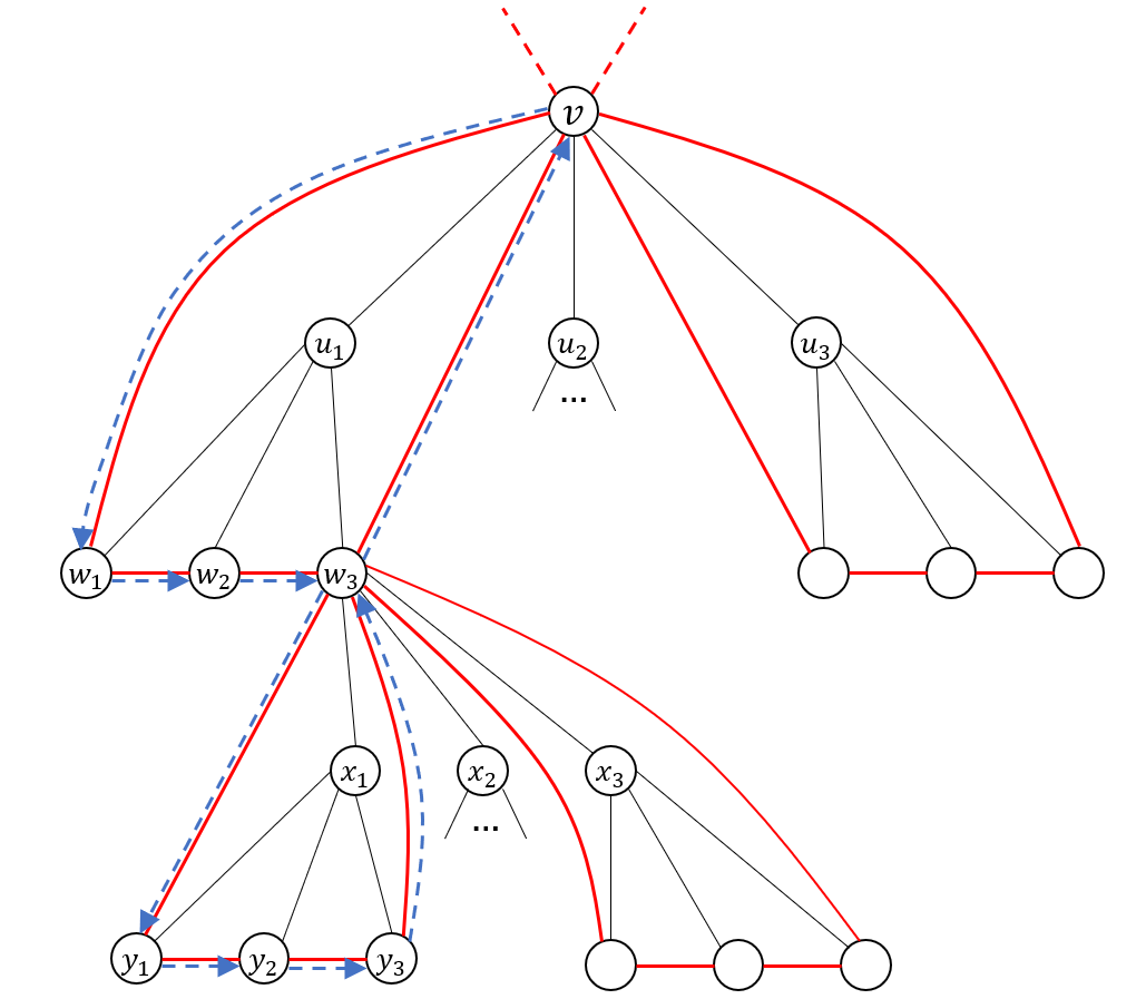
To see this, remember that each child of the root positions the root within a copy of . Therefore, when describing a non-empty cycle originating at the root, we first select one of its children, which determines the copy of in which the root is involved. Now, consider any cycle within that copy of starting at the root, . This cycle corresponds to a cycle in that begins at the root in the following manner: After each step on the cycle, we examine the copy of rooted at and attach a cycle from that copy of . When we return to , we proceed with . Note that attaching an empty cycle is permissible, even though it is not included in , leading to the addition of the neutral element in Equation 3.1. Furthermore, after the final step , we attach another (potentially empty) copy of to account for cycles that visit the root more than twice. This rationale underpins our definition of , which is designed to prevent over-counting that would have otherwise occur.
Equation 3.1 directly implies that the generating function, , associated with the class satisfies
| (3.2) |
where is the generating function corresponding to the class . On its own, this result does not provide much insight, as the functional equation tends to be intricate, hindering our ability to extract the coefficients of . For instance, even in the simple case of a length- cycle, , in which case , Equation 3.2 takes the form
where the term is a shorthand for , resulting in a complicated expression for .
To address this challenge, we leverage a deep result from analytic combinatorics. We provide the essential background in the full version of the paper. Subsequently, in Section 3.1.3, we will outline our approach to estimating the coefficients of using Equation 3.2 as our starting point.
3.1.2 A brief introduction to analytic combinatorics
The symbolic method classifies combinatorial classes into schemes based on their shared structures. This approach aims to consolidate solutions to these problems and highlight their interrelations. A notable schema within this framework is termed smooth inverse-function schema. These are classes whose generating function satisfies the functional equation , namely, , for some “well-behaved” function . By manipulating Equation 3.2, we see that is tightly connected to this schema. Indeed, letting we have that , where
| (3.3) |
Analytic combinatorics provides a method to estimate the coefficients of the generating function for smooth inverse-function schema. This approach is applicable under certain technical conditions on , which we hide under the rug in this informal proof overview. The key requirement though is that there is a real positive solution to the characteristic equation within -s analytic domain around the origin. To denote the ’th coefficient of a function we use the coefficient extractor operator, . For an analytic function , we have
With this, we have the following theorem which is informally stated here (see the full version of the paper for the formal statement).
Theorem 7.
Let belong to the smooth inverse-function schema. Then, with the positive root of the corresponding characteristic equation , one has
| (3.4) |
3.1.3 Proof sketch of Theorem 1
With Theorem 7 in hand, and by the discussion above that led us to Equation 3.3, we are ready to sketch the proof of Theorem 1. In fact, it will be more convenient to consider the variant using the Cauchy transform of . Since , we have that . It can also be shown that (see the full version of the paper for the proof), and so Equation 3.3 takes on the form
Through some algebraic manipulations, it becomes evident that the characteristic equation, , transforms into the form presented in Equation 2.5 from Theorem 2 when is substituted with its reciprocal. Specifically, the equation becomes
Upon further analytical exploration, it can be shown that this equation has a positive real root . Consequently, there exists a positive , where , that satisfies the characteristic equation. This allows us to apply Theorem 7 and derive the sought-after estimate
3.2 Matching the lower bound with -local graphs
As briefly discussed in Section 2.2, the proof of Theorem 3 makes use of finite free probability. Thus, to start with, in Section 3.2.1 we give a brief account of this elegant theory. Then, in Section 3.2.2 we sketch the proof of Theorem 3.
3.2.1 Finite free probability
Free probability is a branch of mathematics, initiated by Voiculescu, that extends classical probability theory into the non-commutative setting. In classical probability, random variables are analyzed using their joint distribution, which encodes the correlations or lack of between them. In contrast, free probability introduces the abstract notion of “freeness” to represent the absence of correlations, appropriately defined, among non-commutative random variables. Free probability theory provides, in particular, tools to analyze the spectrum of the sum and product of two operators, given that these operators are free, using knowledge of their individual spectra. Freeness is an infinite-dimensional phenomena in the sense that a pair of finite-dimensional operators can only be free from one another if one of them is constant. As a result, operators associated with finite graphs cannot be studied directly by free probability theory.
In response to this limitation, Marcus, Spielman, and Srivastava, in their groundbreaking series of works [21, 22, 23], introduced the theory of finite free probability along with the associated technique of interlacing. This enabled them to extend some results of free probability to the finite-dimensional setting, especially regarding the spectra of matrix sums and products. While finite free probability may not capture all details of the latter spectra, it provides a one-sided bound on its support. Finite free probability does not depend on the abstract concept of freeness or any analogous notion. Rather, it demonstrates that conjugating a finite operator, , with an orthogonal matrix – sampled according to the Haar measure on this group – effectively “frees” from other operators. We consider a specific application of this principle in the context of operator addition.
Definition 8 (Definition 2.4 in [22]).
Let be real symmetric matrices, with characteristic polynomials and , respectively. The additive convolution of and is defined as
| (3.5) |
where the expectation is taken over random orthogonal matrices sampled according to the Haar measure on the group of -dimensional orthogonal matrices.
We note that, while it may not be immediately apparent, the right-hand side of Equation 3.5 depends only on the spectra of and . Consequently, the additive convolution is well-defined. It was also proved in [23] that is real-rooted itself, hence a discussion of bounding its roots is sensible. When is clear from context, we omit the subscript in .
The analytic machinery that will allow us to study the additive convolution is the Cauchy transform and its max-inverse (see the full version for details). More precisely, the Cauchy transform of a real-rooted degree polynomial , whose roots are , is defined as Clearly, for an undirected graph , the Cauchy transform as defined in Equation 2.4 can be expressed as where is the characteristic polynomial of .
Note that when the Cauchy transform of a polynomial is restricted to the domain to the right of its rightmost pole, , its range is . Additionally, is monotonically decreasing within this domain. With this in mind, one can define to be the inverse of when restricted to the latter domain. In other words, is the max-inverse of . Particularly, for every , provides an upper bound on the largest root, , of . The key feature of the -transform is that it behaves very-well under additive convolution.
Theorem 9 (Theorem 1.12 in [23]).
For all real symmetric matrices with characteristic polynomials , respectively, and for every , it holds that
It is worth noting that in free probability, the analog statement to Theorem 9 in the infinite dimensional case holds with equality.
3.2.2 Proof sketch of Theorem 3
The main idea in proving Theorem 3 is to randomly construct an -local graph in a very intuitive way: since we want each vertex to appear in instances of , we place in such instances, choosing the neighbors uniformly at random. Formally, we define a matrix consisting of disjoint copies of , and sum random permutations of this matrix. This results in the matrix
where are permutation matrices. The proof for the existence of an -local graph whose second largest eigenvalue meet our lower bound incorporates two parts:
-
1.
Bounding the second largest root of the expected characteristic polynomial, , where the permutations are sampled uniformly and independently at random.
-
2.
Relating the roots of to roots of a particular choice for , resulting in finding a good permutation, which induces a graph.
On first sight, it is not clear how to relate the expectation polynomial from Part 1 with the aforementioned tools of finite free probability. Definition 8 uses an expectation over the Haar measure, and together with Theorem 9 (applied times) enables us to establish an upper bound on the largest root of the expected characteristic polynomial, derived as the “free sum” of of identical matrices. More precisely, a corollary from Theorem 9, together with the above discussion, yields
| (3.6) |
where is the largest eigenvalue of . When taking to be the matrix , the RHS of Equation 3.6 resembles Equation 2.6 from Theorem 2. However, the relevance of the LHS of the above equation remains unclear, as the expectation hidden in the operation is over the Haar measure and not over permutations. For bridging this gap, as well as for establishing Part 2, we follow MSS and proceed in two steps: quadrature and interlacing. While our proof makes a black-box use of these techniques we believe that the unfamiliar reader will benefit from this short account.
Quadrature
Quadrature refers to a general technique by which an integral is written as a finite sum. In our context, we make use of the result showing that finite free additive convolution can be expressed using the finite subgroup of permutation matrices of the unitary group. Specifically,
Theorem 10 (Theorem 4.1 in [22]).
Let be symmetric matrices with and . Let and . Then,
where is a uniformly random permutation matrix.
Assume that is the adjacency matrix of a -regular graph, and let . As a direct corollary of Theorem 10, we get that
Consequently, by taking , the upper bound on the max-root of the convolution polynomial, derived using Equation 3.6, directly establishes a bound on the max-root of the expected characteristic polynomial appearing on the LHS. The advantage is that we are now considering an expectation over a finite distribution, and more importantly, each element in the support of the distribution is an -local graph. The final step of interlacing permits us to conclude that an element exists within this distribution for which the same upper bound holds.
Interlacing
So far, we have discussed how to obtain a bound on the largest root of the expected characteristic polynomial (excluding the trivial root), where the expectation is over the group of permutation matrices. It is generally incorrect to assert that a bound on the largest root of the expectation of polynomials can be utilized to infer a bound on the largest root of one of the polynomials involved in the expectation. A key observation by MSS concerning this issue is that such an result holds if the polynomials participating in the expectation form an interlacing family. In fact, for any choice of , this structure suffices to deduce a bound on the -th largest root of at least one polynomial in the family, given that we are able to bound the -th largest root of the expected characteristic polynomial.
4 Derandomized Squaring with Interesting Graphs
In this section we apply our results to some interesting graph families, starting with graphs which demonstrate the tightness of our lower bound (see Section 4.1). Our general bound on bounded-degree graphs is given in Section 4.2 and the stronger bound assuming good spectral expansion is given in Section 4.3. The complete bipartite graph is studied in Section 4.4. The remaining sections deal with Paley graphs (see Section 4.5) and, more generally, strongly regular graphs (see Section 4.6), as well as some specific interesting graphs in Section 4.7. Some of the proofs of the results are omitted and can be found in the full version of the paper.
4.1 Three tight examples
In this short section we analyze some basic choices for the graph , for which we know what behavior to expect and compare against our bound. We prove that for these instances, our lower bound given by Theorem 2 is tight, up to an additive vanishing term, for every Ramanujan graph .
4.1.1 The true square
Let be a -regular graph, where , and let denote the complete graph on vertices, self-loops included. That is, is the graph whose adjacency matrix is the all-ones matrix, typically denoted as . Note that . Our lower bound on obtained in Theorem 2 holds for all graphs in the sense that is independent of . Therefore, it is sensible to expect that if the lower bound is tight for this choice of then it is matched by taking to be a -regular Ramanujan graph. In such case, the spectral expansion can be computed directly and is equal to . As we will now show, it is indeed the case that , establishing that our lower bound is tight for this choice of .
The Cauchy transform of is given by
Substituting to Equation 2.5 and simplifying, we see that the derandomized squaring polynomial associated with is given by The unique real positive root of is, of course . Substituting to Equation 2.6 yields .
4.1.2 Non-backtracking random walks
A second example for the tightness of our bound is given by the clique, denoted as , namely the complete graph without self-loops. It is easily seen combinatorially that corresponds to the graph of non-backtracking length- walks in , which we denote by . The corresponding adjacency matrix is given by . Hence, for a Ramanujan graph , the best value we can hope for coming from the analysis is
This bound is indeed what results from our analysis. To see this, note that the Cauchy transform of is
Substituting to Equation 2.5 and simplifying, we see that the derandomized squaring polynomial associated with is given by
The unique real positive root of is . Substituting to Equation 2.6 yields the desired bound, .
It is instructive to compare our bound with the upper bound obtained by the Rozenman-Vadhan bound, Equation 1.1 for a Ramanujan graph . The second largest (normalized) eigenvalue of in absolute value is , leading to an overall bound of compared to the true behavior of .
4.1.3 The graph achieving the Rozenman-Vadhan bound
In [35], Rozenman and Vadhan proved that the bound that is given in Equation 1.1 is tight in a strong sense, namely, for every rational , there exists a graph with , such that for every graph it holds that . For ease of notation, we write instead of from hereon. The graph is constructed as follows: assume for some integers , then is a graph on vertices which is -regular, consisting of copies of the complete graph , and additional self-loops on each vertex. The combinatorial analysis shows that a step in the -regular graph amounts to staying at the same vertex with probability or taking a step in with probability , leading directly to the tightness of the bound.
Assume once again that is Ramanujan, hence . In this case, by Equation 1.1, we get that
As in the above two examples, we use the Cauchy transform of which is given by
Expanding Equation 2.7 and solving, we get
as in the Rozenman-Vadhan bound.
4.2 Bounded-degree graphs and a universal bound on
In this section we prove that derandomized squaring with a simple vertex-transitive graph of bounded degree results with a graph that gravitates towards Ramanujan as the number of vertices in increases. Moreover, we establish a universal bound on which holds for all simple vertex-transitive graphs.
Theorem 11.
Let be a simple vertex-transitive -regular graph on vertices, where and . Then,
Moreover, for every it holds that . Lastly, if is triangle-free then
4.3 Spectral expanders
In this section we prove a stronger bound on than the one obtained in Theorem 11, which recall holds for general bounded-degree graphs, assuming that is a good spectral expander. The proof follows the same argument as in the proof of Theorem 11 though takes into account the bound on the spectral expansion.
Proposition 12.
Let be a simple vertex-transitive -regular graph on vertices. Assume that . Then,
Furthermore, if is triangle-free then
4.4 Complete bipartite graphs
In this section we consider the operation of derandomized squaring with the complete bipartite graph on vertices, for an even integer . This is, of course, a regular graph which we denote as . It is easy to see that has eigenvalues , each with multiplicity , and the remaining eigenvalues are all . Therefore, the corresponding Cauchy transform, which for ease of notation we denote by , is given by
From here one can compute the derandomized squaring polynomial
whose unique positive root where One can verify that Substituting this to Equation 2.6, we get
The resulted graph is -regular, and so we normalize by dividing by to get
From here one can compute the first couple of values, which, of course, matches the bound we computed for the length- cycle, and . Considering the limit behavior as we have that where , and so
4.5 Paley graphs
Let be a prime power. The Paley graph, denoted as , has vertex set corresponding to the finite field with the vertices adjacent if and only if their difference is a nonzero square in . As modulo , we have that is a square in , and so is undirected.
Theorem 13.
4.6 Strongly regular graphs
A -regular graph on vertices with no self-loops is called strongly regular with parameters 444It is customary to denote these parameters by and and so, despite our use of for denoting the spectral expansion, we proceed with this standard notation. if (namely, the graph is neither complete nor edgeless) and the following hold:
-
1.
For each pair of adjacent vertices there are vertices adjacent to both.
-
2.
For each pair of nonadjacent vertices there are vertices adjacent to both.
Strongly regular graphs include dozens of interesting graphs such as the Peterson graph, the Hoffman-Singelton graph (see Section 4.7), and the symplectic graphs (see Section 4.6.1), as well as all Paley graphs which we analyzed in Section 4.5. It is a well-known fact that strongly regular graphs have two eigenvalues other than the trivial eigenvalue , denoted , with the convention . This is, in fact, a spectral characterization of strongly regular graph among regular graphs. The multiplicity of these eigenvalues are denoted by , respectively. In the following we compute the derandomized squaring polynomial of a strongly regular graph.
Proposition 14.
Let be a -regular strongly regular graph on vertices with parameters . Let and . Then, the derandomized squaring polynomial associated with is given by
where
4.6.1 The symplectic graphs
An interesting sub-family of strongly regular graphs are the so-called symplectic graphs. Let be an integer. The symplectic graph is the graph whose vertex set consists of all nonzero vectors in . Two vertices are adjacent whenever , with all calculations over , where is the block diagonal matrix with blocks of the form . It is well-known that is a strongly regular graph with .
Theorem 15.
Interestingly, though not unexpectedly, this limit behavior is also shared by Paley graphs (see Section 4.5).
4.7 Some specific graphs
In this section we consider some specific interesting graphs.
| (Graph name) | (Number of vertices) | (degree) | |
|---|---|---|---|
| Petersen graph | 10 | 3 | 2.025 |
| Heawood graph | 14 | 3 | 2.004 |
| Hoffman-Singelton graph | 50 | 7 | 2.007 |
| Biggs-Smith graph | 102 | 3 | 2.000000016 |
| Conway’s 99-graph | 99 | 14 | 2.041 |
References
- [1] AmirMahdi Ahmadinejad, Jonathan Kelner, Jack Murtagh, John Peebles, Aaron Sidford, and Salil Vadhan. High-precision estimation of random walks in small space. In 2020 IEEE 61st Annual Symposium on Foundations of Computer Science, pages 1295–1306. IEEE Computer Soc., Los Alamitos, CA, [2020] ©2020. doi:10.1109/FOCS46700.2020.00123.
- [2] AmirMahdi Ahmadinejad, John Peebles, Edward Pyne, Aaron Sidford, and Salil Vadhan. Singular value approximation and reducing directed to undirected graph sparsification. arXiv preprint arXiv:2301.13541, 2023. doi:10.48550/arXiv.2301.13541.
- [3] N. Alon and F. R. K. Chung. Explicit construction of linear sized tolerant networks. In Proceedings of the First Japan Conference on Graph Theory and Applications (Hakone, 1986), volume 72, pages 15–19, 1988. doi:10.1016/0012-365X(88)90189-6.
- [4] Noga Alon. Eigenvalues and expanders. Combinatorica, 6(2):83–96, 1986. doi:10.1007/BF02579166.
- [5] Avraham Ben-Aroya and Amnon Ta-Shma. A combinatorial construction of almost-Ramanujan graphs using the zig-zag product. SIAM J. Comput., 40(2):267–290, 2011. doi:10.1137/080732651.
- [6] Yonatan Bilu and Nathan Linial. Lifts, discrepancy and nearly optimal spectral gap. Combinatorica, 26(5):495–519, 2006. doi:10.1007/s00493-006-0029-7.
- [7] Charles Bordenave. A new proof of Friedman’s second eigenvalue theorem and its extension to random lifts. Ann. Sci. Éc. Norm. Supér. (4), 53(6):1393–1439, 2020. doi:10.24033/asens.2450.
- [8] Charles Bordenave and Benoît Collins. Eigenvalues of random lifts and polynomials of random permutation matrices. Annals of Mathematics, 190(3):811–875, 2019.
- [9] Mark Braverman, Gil Cohen, and Sumegha Garg. Pseudorandom pseudo-distributions with near-optimal error for read-once branching programs. SIAM Journal on Computing, 49(5):STOC18–242, 2019. doi:10.1137/18M1197734.
- [10] Eshan Chattopadhyay and Jyun-Jie Liao. Optimal error pseudodistributions for read-once branching programs. In 35th Computational Complexity Conference, volume 169 of LIPIcs. Leibniz Int. Proc. Inform., pages Art. No. 25, 27. Schloss Dagstuhl – Leibniz-Zentrum für Informatik, 2020. doi:10.4230/LIPICS.CCC.2020.25.
- [11] Lijie Chen, William Hoza, Xin Lyu, Avishay Tal, and Hongxun Wu. Weighted pseudorandom generators via inverse analysis of random walks and shortcutting. In Electronic Colloquium on Computational Complexity (ECCC), volume 114, 2023.
- [12] Gil Cohen and Gal Maor. Random walks on rotating expanders. In Proceedings of the 55th Annual ACM Symposium on Theory of Computing, pages 971–984, 2023. doi:10.1145/3564246.3585133.
- [13] Michael B. Cohen. Ramanujan graphs in polynomial time. In 57th Annual IEEE Symposium on Foundations of Computer Science—FOCS 2016, pages 276–281. IEEE Computer Soc., Los Alamitos, CA, 2016. doi:10.1109/FOCS.2016.37.
- [14] Joel Friedman. A proof of Alon’s second eigenvalue conjecture and related problems. Mem. Amer. Math. Soc., 195(910):viii+100, 2008. doi:10.1090/memo/0910.
- [15] Rostislav I Grigorchuk and Andrzej Zuk. On the asymptotic spectrum of random walks on infinite families of graphs. Random walks and discrete potential theory (Cortona, 1997), pages 188–204, 1999.
- [16] Chris Hall, Doron Puder, and William F. Sawin. Ramanujan coverings of graphs. Adv. Math., 323:367–410, 2018. doi:10.1016/j.aim.2017.10.042.
- [17] Shlomo Hoory, Nathan Linial, and Avi Wigderson. Expander graphs and their applications. Bulletin of the American Mathematical Society, 43(4):439–561, 2006.
- [18] Yasutaka Ihara. On discrete subgroups of the two by two projective linear group over p-adic fields. J. Math. Soc. Japan, 18:219–235, 1966. doi:10.2969/jmsj/01830219.
- [19] Alexander Lubotzky, Ralph Phillips, and Peter Sarnak. Ramanujan graphs. Combinatorica, 8(3):261–277, 1988. doi:10.1007/BF02126799.
- [20] Adam W. Marcus, Daniel A. Spielman, and Nikhil Srivastava. Interlacing families I: Bipartite Ramanujan graphs of all degrees. Ann. of Math. (2), 182(1):307–325, 2015. doi:10.4007/annals.2015.182.1.7.
- [21] Adam W. Marcus, Daniel A. Spielman, and Nikhil Srivastava. Interlacing families II: Mixed characteristic polynomials and the Kadison-Singer problem. Ann. of Math. (2), 182(1):327–350, 2015. doi:10.4007/annals.2015.182.1.8.
- [22] Adam W Marcus, Daniel A Spielman, and Nikhil Srivastava. Interlacing families IV: Bipartite Ramanujan graphs of all sizes. SIAM Journal on Computing, 47(6):2488–2509, 2018. doi:10.1137/16M106176X.
- [23] Adam W. Marcus, Daniel A. Spielman, and Nikhil Srivastava. Finite free convolutions of polynomials. Probab. Theory Related Fields, 182(3-4):807–848, 2022. doi:10.1007/s00440-021-01105-w.
- [24] Grigorii Aleksandrovich Margulis. Explicit group-theoretical constructions of combinatorial schemes and their application to the design of expanders and concentrators. Problemy peredachi informatsii, 24(1):51–60, 1988.
- [25] Sidhanth Mohanty and Ryan O’Donnell. -Ramanujan graphs. In Proceedings of the 2020 ACM-SIAM Symposium on Discrete Algorithms, pages 1226–1243. SIAM, Philadelphia, PA, 2020. doi:10.1137/1.9781611975994.75.
- [26] Sidhanth Mohanty, Ryan O’Donnell, and Pedro Paredes. Explicit near-Ramanujan graphs of every degree. SIAM J. Comput., 51(3):1–23, 2022. doi:10.1137/20M1342112.
- [27] Moshe Morgenstern. Existence and explicit constructions of regular Ramanujan graphs for every prime power . J. Combin. Theory Ser. B, 62(1):44–62, 1994. doi:10.1006/jctb.1994.1054.
- [28] Jack Murtagh, Omer Reingold, Aaron Sidford, and Salil Vadhan. Derandomization beyond connectivity: undirected Laplacian systems in nearly logarithmic space. SIAM J. Comput., 50(6):1892–1922, 2021. doi:10.1137/20M134109X.
- [29] Alexandru Nica and Roland Speicher. Lectures on the combinatorics of free probability, volume 335 of London Mathematical Society Lecture Note Series. Cambridge University Press, Cambridge, 2006. doi:10.1017/CBO9780511735127.
- [30] A. Nilli. On the second eigenvalue of a graph. Discrete Math., 91(2):207–210, 1991. doi:10.1016/0012-365X(91)90112-F.
- [31] Ryan O’Donnell and Xinyu Wu. Explicit near-fully X-Ramanujan graphs. In 2020 IEEE 61st Annual Symposium on Foundations of Computer Science, pages 1045–1056. IEEE Computer Soc., Los Alamitos, CA, 2020.
- [32] Karol A Penson and Karol Życzkowski. Product of ginibre matrices: Fuss-Catalan and Raney distributions. Physical Review E, 83(6):061118, 2011.
- [33] Omer Reingold. Undirected connectivity in log-space. J. ACM, 55(4):Art. 17, 24, 2008. doi:10.1145/1391289.1391291.
- [34] Omer Reingold, Salil Vadhan, and Avi Wigderson. Entropy waves, the zig-zag graph product, and new constant-degree expanders and extractors. In Proceedings 41st Annual Symposium on Foundations of Computer Science, pages 3–13. IEEE, 2000. doi:10.1109/SFCS.2000.892006.
- [35] Eyal Rozenman and Salil Vadhan. Derandomized squaring of graphs. In Approximation, randomization and combinatorial optimization, volume 3624 of Lecture Notes in Comput. Sci., pages 436–447. Springer, Berlin, 2005. doi:10.1007/11538462_37.
- [36] Amnon Ta-Shma. Explicit, almost optimal, epsilon-balanced codes. In Proceedings of the 49th Annual ACM SIGACT Symposium on Theory of Computing, pages 238–251, 2017. doi:10.1145/3055399.3055408.
- [37] Wolfgang Woess. Random walks on infinite graphs and groups, volume 138 of Cambridge Tracts in Mathematics. Cambridge University Press, Cambridge, 2000. doi:10.1017/CBO9780511470967.