Error-Correcting Graph Codes

Similar to the Hamming setting, we briefly define the dimension, rate, and distance of a graph code $C$ on $n$ vertices where each edge is allowed to have an arbitrary symbol $\alpha \in {𝔽}_q$ written on it.

• $\mathrm{■}$

  Dimension. $k={\log }_q(|C|)$.

• $\mathrm{■}$

  Rate. $R={\log }_q(|C|)/\left(\genfrac{}{}{0pt}{}{n}{2}\right)$.

• $\mathrm{■}$

  Distance. The distance of a code is the largest $d$ such that ${\mathrm{d}}_{\mathrm{graph}}(G,H)\ge d$ for each $G,H\in C$ such that $G\ne H$. The relative distance $\delta$ is $d/n$.

Unless specified otherwise , we will always be interested in asymptotics of the above parameters as $n\to \mathrm{\infty }$.

As noted in [19], an argument similar to the Singleton bound states that for a graph code of dimension $k$, and distance $d$, we have

In terms of and rate $R$, and relative distance $\delta$, we have

A code is called optimal if it $R\sim {(1-\delta )}^2$, equivalently, $\delta \sim 1-\sqrt{R}$.

The relevant constructions in [19], [18] are summarized in Table 1. Note that all of the constructions in Table 1 are for undirected graphs where self-loops are allowed. One can impose $n$ linear constraints to get codes with no self-loops (zeros on the diagonals of the adjacency matrix). Since the block length of these codes is $\left(\genfrac{}{}{0pt}{}{n}{2}\right)$, adding these these constraints changes the rate by $o(1)$.

Construction 5 of [19] leverages a connection to symmetric array codes and construction by Schmidt [15]. The trade-off achieved, $R\sim 1-2\delta$ is close to optimal for $\delta$ very small.

Construction 3 of [19] translates Hamming distance into graph distance using the tensor product. Although this construction doesn’t directly imply anything about binary codes due to the requirement on field size, a similar code will be an important ingredient in our constructions.

Our main results are:

1. 1.

   We show that there are optimal binary codes for any constant $\delta \in (0,1)$.

2. 2.

   We give constructions of graph codes that have positive constant $R$ for all constant . In particular, we give a quasi-polynomial time explicit construction achieving $\delta =1-O(R^{1/4})$, while optimal codes have $\delta =1-R^{1/2}$. We also give an explicit construction with $\delta =1-O(R^{1/6})$, and a strongly explicit construction with $\delta =1-O(R^{1/8})$. Although these codes are not optimal, they are the first binary error-correcting graph codes achieving $\delta >1/2$ with a constant rate.

3. 3.

   We give (strongly) explicit constructions of graph codes with very high $\delta =1-O(n^{-ϵ})$ and $R=\mathrm{\Omega }(n^{ϵ-1/2})$ for constant $ϵ>0$. This gives a “graph code of Ramsey graphs” as will be discussed later.

We now discuss our techniques. We will often specify graphs by their adjacency matrices, viewed as matrices with ${𝔽}_2$ entries.

Our nonconstructive existence result is a straightforward application of the probabilistic method. We consider a uniformly random ${𝔽}_2$-linear subspace of the ${𝔽}_2$-linear space of symmetric $0$-diagonal $n\times n$ matrices (i.e., the space of all adjacency matrices of graphs); this turns out to give a good graph code with optimal $R$ vs $\delta$ tradeoff. Such graph codes can be specified by an ${𝔽}_2$ basis for it. We say that a construction is explicit if this basis can be produced in $\text{poly}(n)$ time. We say it is strongly explicit if, given $(i,j,k)$, the $(i,j)$ entry of the $k$’th basis element can be computed in $\text{poly}(\log (n))$ time.

To get asymptotically good codes for any constant $\delta \in (0,1)$ we take a longer detour.

1. 1.

   We start with a slight variation of [19] (Construction 3), which gives a way to get a good graph code from a classical Hamming-distance linear code $C\subseteq {𝔽}_2^n$. We first consider the tensor code $C\otimes C$, where the elements are matrices all of whose rows and columns are codewords of $C$. A-priori, $C$ could contain matrices that are neither symmetric, not have a $0$ diagonal. But interestingly, if we consider the set $C^{\ast }$ of all matrices in $C\otimes C$ that are symmetric and have $0$ diagonal, then $C^{\ast }$ is a linear space with quite large dimension. In particular, if the classical Hamming distance code $C$ has positive rate, then so does the graph code $C^{\ast }$. We call this construction $C^{\ast }=\mathrm{STCZD}(C)$ (Symmetric Tensor Code with Zero Diagonals).

   It turns out that if $C$ has good relative distance (in the Hamming metric), then $\mathrm{STCZD}(C)$ has good distance in the graph metric. However the relative graph distance of $\mathrm{STCZD}(C)$ such a code is bounded by the relative distance of $C$ – and since $C$ is a binary code, this is at most $1/2$.

2. 2.

   Now, we bring in another idea from the Hamming code world: code concatenation. Instead of constructing a graph code of symmetric zero-diagonal matrices over ${𝔽}_2$, we instead construct a “large-alphabet graph code” of symmetric zero-diagonal matrices over ${𝔽}_q$ for some large $q=2^t$ and then try to reduce the alphabet size down to $2$ by replacing the $q$-ary symbols with ${𝔽}_2$-matrices with suitable properties.

   Applying the analog of $\mathrm{STCZD}$ to a large alphabet code allows one to get large-alphabet graph codes with large $\delta$, approaching $1$ (since over large alphabets Hamming distance codes can have length approaching $1$). Using Reed-Solomon codes as these large alphabet codes also allows us to make the $\mathrm{STCZD}$ construction strongly explicit. Furthermore, when applied to Reed-Solomon codes, these codes have a natural direct description: these are the evaluation tables of low-degree bivariate polynomials $P(X,Y)$ on product sets $S\times S$ that are (1) symmetric (to get a symmetric matrix), and (2) multiples of ${(X-Y)}^2$ (to get zero diagonal).

3. 3.

   What remains now is to develop the right kind of concatenation so that the resulting graph code has good distance. This turns out to be subtle and requires an “inner code” with a stronger “directed graph distance” property with $\delta$ nearly 1. Fortunately, this inner code we seek is of very slowly growing size, and we may find this by brute force search. This concludes our description of our explicit construction of graph codes with $\delta$ approaching $1$ and positive constant $R$.

Finally, we discuss our constructions for very high distances, $\delta =1-o(1)$. In this regime, as mentioned earlier, this is related to constructions of Ramsey graphs, a difficult problem in pseudorandomness with a long history. Our constructions work up to $\delta =1-\mathrm{\Omega }\left(\frac{1}{\sqrt{n}}\right)$; concretely, we get a large linear space of graphs such that all graphs in the family have no clique or independent set of size $\mathrm{\Omega }(\sqrt{n})$. The construction is based on polynomials over finite fields of characteristic $2$: When $n=2^t$, we consider a linear space of certain low degree univariate polynomials $f(X)$ over ${𝔽}_{2^t}$, and create the ${𝔽}_2$ matrix with rows and columns indexed by ${𝔽}_{2^t}$ whose $x,y$ entry is $\mathrm{𝖳𝗋}(f(x+y))$. Here $\mathrm{𝖳𝗋}$ is the finite field trace map from ${𝔽}_{2^t}$ to ${𝔽}_2$. The use of $\mathrm{𝖳𝗋}$ of polynomials is inspired by the construction of dual-BCH codes. We then show that any such matrix has no large clique or independent set unless $\mathrm{𝖳𝗋}\circ f$ is identically $0$ or identically $1$ (corresponding to the empty and complete graphs respectively). The proof uses the Weil bounds on character sums and a Fourier analytic approach to bound the independence number for the graphs. Our constructions are listed in Table 2.

The most interesting question in this context is to obtain explicit constructions of graph codes with optimal $R$ vs $\delta$ tradeoff. While we have several constructions achieving nontrivial parameters in various regimes, it would even be interesting to get the right asymptotic behavior for the endpoints with $\delta$ approaching $1$. The setting of large $\delta$ (including $\delta =1-o(1)$) seems especially challenging, given the connection with the notorious problem of constructing Ramsey graphs.

Another interesting question is to get decoding algorithms for graph codes. For a certain graph code $C$, if we are given a graph that is promised to be close in graph distance to some graph $G$ in $C$. Then, can we efficiently find $G$?

A more general context relevant to error-correcting graph codes is the error correction of strings under more general error patterns. Suppose we have a collection of subsets $S_i\subseteq [m]$ for $i\in [t]$, where ${\bigcup }_i{S}_i=[m]$. These $S_i$ denote the corruption zones; a single “corruption” of a string $z\in {\{0,1\}}^m$ entails, for some $i\in [t]$, changing ${z|}_{S_i}$ to something arbitrary in ${\{0,1\}}^{S_i}$. We want to design a code $C\subseteq {\{0,1\}}^m$ such that starting at any $x\in C$ if we do fewer than $d$ corruptions to $x$, we do not end up at any $y\in C$ with $y\ne x$. When the $S_i$ are all of size $b$ and form a partition of $[m]$ into $t=m/b$ parts, then such a code is exactly the same as a classical Hamming distance code an alphabet of size $2^b$. Error-correcting graph codes give a first step into the challenging setting where the $S_i$ all pairwise intersect - here we have $m=\left(\genfrac{}{}{0pt}{}{n}{2}\right)$, $t=n$, the $S_i$ (which correspond to all edges incident on a given vertex) all have size $n-1$, and every pair $S_i$ and $S_j$ intersect in exactly $1$ element. It would be interesting to develop this theory – to both find the limits of what is achievable and to develop techniques for constructing codes against this error model.

Finally, there are many other themes from classical coding theory that could make sense to study in the context of graph codes and graph distance, including in the context of sublinear time algorithms. It would be interesting to explore this.

Since our inner code is not guaranteed to be symmetric, simply replacing each field element in the outer code with its encoding might result in an asymmetric matrix. To remedy this, we transpose the encoding for entries below the diagonal. This is made formal below.

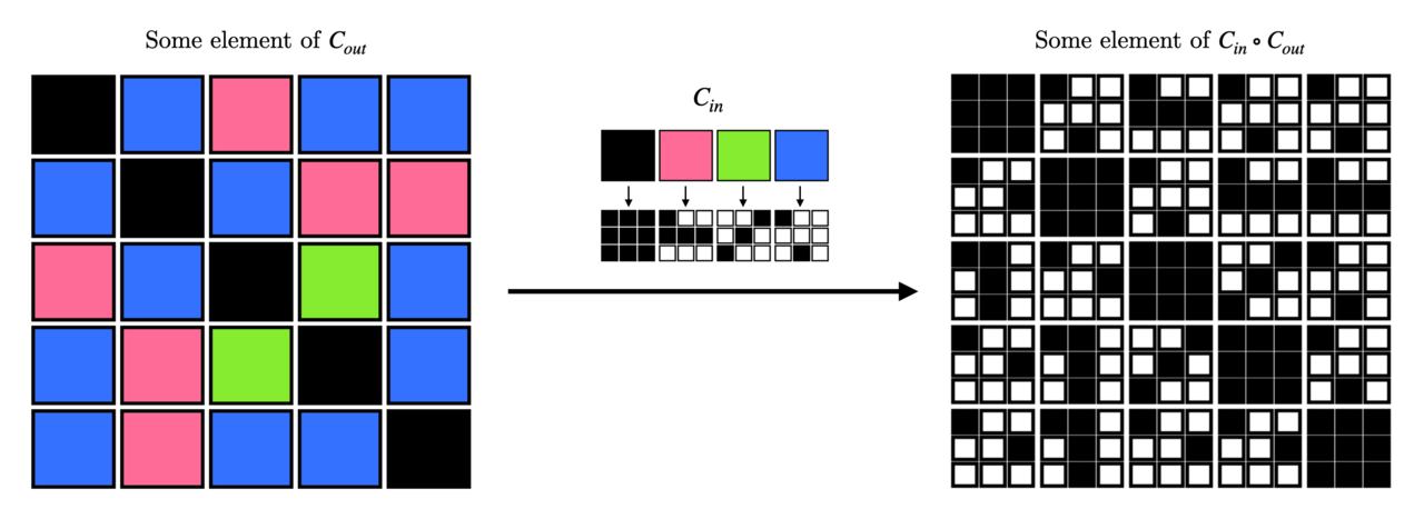
Figure 1 visualizes an example of symmetric concatenation. We now show that distance and dimension concatenate exactly like it does for standard error-correcting codes.

We can instantiate the concatenated code using Reed Solomon codes.

The following theorem follows directly from Lemmas 10 and 17. As a reminder, here we are considering the rate of the codes as a (undirected) graph code.

Note that using this construction, we can get asymptotically good codes for any constant rate and distance - including for distances $>1/2$, which was not obtained in any of the previous constructions. We get $R={(1-\sqrt{\delta })}^4-o(1)$ by setting $ϵ=\rho$.

One drawback of this construction is that it is not strongly explicit or even explicit. The outer code can be made strongly explicit using Lemma 13, however, the inner code was an optimal code which we obtained by a randomized construction. The complexity of searching for such a code by brute force is too large. In particular, the optimal code has dimension ${ϵ}^2{n}^2$, and block length $n^2$. Since we need the size of the code to be equal to the size of the outer alphabet, we have $N=2^{{ϵ}^2{n}^2}$, so $n=\sqrt{\log (N)}/ϵ$. Then, there are at least $2^{{ϵ}^2{n}^4}=2^{\log {(N)}^2/{ϵ}^2}$ generator matrices to search over. Thus, we cannot find such a code efficiently.

To address this, we reduce the search space by concatenating multiple times. The resulting code will have a slightly worse distance/rate tradeoff but will still be asymptotically good for any constant distance or rate.

We also note that $C_{\mathrm{RS}}$ can also be made strongly explicit using a Justensen-like construction. However, although this code is again asymptotically good, it has distance bounded away from 1. We present this construction in the Appendix.

While concatenating twice suffices to obtain an explicit code, it is not clear that the obtained code is strongly explicit. This may be addressed by concatenating three times, at the cost of slightly weaker parameters. Here, we will also use the tensor product code as a building block. For any linear code $C\subset {𝔽}_q^n$ let $\mathrm{TC}(C)$ be the tensor product code of $C$. As a reminder, $\mathrm{TC}(C)$ is the code consisting of matrices $A\in {𝔽}_q^{n\times n}$ such that each row and each column of $A$ are elements of $C$.

Below we present the analysis for triple concatenation.

Notice that only the outer-most code needs to be symmetric and have zero diagonal since we use the symmetric concatenation operation (entries below the diagonal will be transposed). Thus, using the Tensor Product Code for the two middle codes (instead of STCZD) is sufficient and saves a factor of 2 (each time) on the rate.

As a warmup, we first construct code with distance $1-\frac{1}{n^{ϵ}}$ with growing dimension.

Let $n=2^t$. Let $\mathrm{𝖳𝗋}:{𝔽}_{2^t}\to {𝔽}_2$ denote the finite field trace map. Concretely, it is given by:

For each $\alpha \in {𝔽}_{2^t}$, consider the matrix $M_{\alpha }\in {𝔽}_2^{n\times n}$, where the rows and columns of $M_{\alpha }$ are indexed by elements of ${𝔽}_{2^t}$, given by:

Note that each $M_{\alpha }$ is symmetric. Consider the code

We have that $C_{\mathrm{Warmup}}$ is a linear code of dimension $t={\log }_{2}n$.

We now see how to get graph codes of distance $1-\frac{1}{n^{ϵ}}$ with and larger rate.

For a polynomial $f(X)\in {𝔽}_{2^t}[X]$, let $M_f$ be $n\times n$ matrix with rows and columns indexed by ${𝔽}_{2^t}$ for which:

Let $W_d$ be the ${𝔽}_{2^t}$-linear space of all polynomials $f(X)$ of the form:

where the ${\alpha }_i\in {𝔽}_{2^t}$.

Then, let us define our construction.

References

- [1] Noga Alon. Connectivity graph-codes. arXiv preprint, 2023. arXiv:2308.07653.
- [2] Noga Alon. Graph-codes. arXiv preprint, 2023. arXiv:2301.13305.
- [3] Noga Alon, Anna Gujgiczer, János Körner, Aleksa Milojević, and Gábor Simonyi. Structured codes of graphs. SIAM Journal on Discrete Mathematics, 37(1):379–403, 2023. doi:10.1137/22M1487989.
- [4] Per Austrin and Subhash Khot. A Simple Deterministic Reduction for the Gap Minimum Distance of Code Problem. IEEE Transactions on Information Theory, 60(10):6636–6645, 2014. doi:10.1109/TIT.2014.2340869.
- [5] Shixi Chen and Shuigeng Zhou. Recursive mechanism: Towards node differential privacy and unrestricted joins. In Proceedings of the 2013 ACM SIGMOD International Conference on Management of Data, SIGMOD ’13, pages 653–664. Association for Computing Machinery, 2013. doi:10.1145/2463676.2465304.
- [6] Pat Devlin. Personal Communication.
- [7] G David Forney. Concatenated codes. Technical report, Massachusetts Institute of Technology, Research Laboratory of Electronics, 1965.
- [8] Michael Hay, Chao Li, Gerome Miklau, and David Jensen. Accurate Estimation of the Degree Distribution of Private Networks. In 2009 Ninth IEEE International Conference on Data Mining, pages 169–178, 2009. doi:10.1109/ICDM.2009.11.
- [9] Palak Jain, Adam Smith, and Connor Wagaman. Time-Aware Projections: Truly Node-Private Graph Statistics under Continual Observation. arXiv, 2024. doi:10.48550/arXiv.2403.04630.
- [10] J. Justesen. Class of constructive asymptotically good algebraic codes. IEEE Transactions on Information Theory, 18(5):652–656, 1972. doi:10.1109/TIT.1972.1054893.
- [11] Shiva Prasad Kasiviswanathan, Kobbi Nissim, Sofya Raskhodnikova, and Adam Smith. Analyzing graphs with node differential privacy. In Proceedings of the 10th Theory of Cryptography Conference on Theory of Cryptography, TCC’13, pages 457–476. Springer-Verlag, 2013. doi:10.1007/978-3-642-36594-2_26.
- [12] James L Massey. Threshold decoding. Technical report, Massachusetts Institute of Technology, Research Laboratory of Electronics, 1963.
- [13] M. Plotkin. Binary codes with specified minimum distance. IRE Transactions on Information Theory, 6(4):445–450, 1960. doi:10.1109/TIT.1960.1057584.
- [14] I. S. Reed and G. Solomon. Polynomial Codes Over Certain Finite Fields. Journal of the Society for Industrial and Applied Mathematics, 8(2):300–304, 1960. doi:10.1137/0108018.
- [15] Kai-Uwe Schmidt. Symmetric bilinear forms over finite fields with applications to coding theory. Journal of Algebraic Combinatorics, 42(2):635–670, 2015. doi:10.1007/s10801-015-0595-0.
- [16] W.M. Schmidt. Equations over Finite Fields: An Elementary Approach. Lecture Notes in Mathematics. Springer Berlin Heidelberg, 2006. URL: https://books.google.co.uk/books?id=up97CwAAQBAJ.
- [17] J. Wolf. On codes derivable from the tensor product of check matrices. IEEE Transactions on Information Theory, 11(2):281–284, 1965. doi:10.1109/TIT.1965.1053771.
- [18] Lev Yohananov, Yuval Efron, and Eitan Yaakobi. Double and Triple Node-Erasure-Correcting Codes Over Complete Graphs. IEEE Transactions on Information Theory, 66(7):4089–4103, 2020. doi:10.1109/TIT.2020.2971997.
- [19] Lev Yohananov and Eitan Yaakobi. Codes for Graph Erasures. IEEE Transactions on Information Theory, 65(9):5433–5453, 2019. doi:10.1109/TIT.2019.2910040.
Appendix A Justensen-like code
The construction in this example is inspired by the Justensen code [10], which uses an ensemble of codes for the inner code instead of a single inner code. Justensen uses an ensemble known as the Wozencraft Ensemble [12] with the following properties.
Theorem 32 (Wozencraft Ensemble).
For every large enough , there exists codes over with rate , where fraction of them have distance at least .
Since our goal is graph distance, we use the operation to covert the Wozencraft Ensemble from codes over strings with good Hamming distance to codes of matrices with good graph distance.
Lemma 33 (Wozencraft Ensemble Modification).
For any , and large enough , there exists codes over . View these as directed graph codes. Then these codes have rate , and at least a fraction of them have distance at least .
Proof.
Let be the Wozencraft Ensemble. For each , define . Note that each is a code over . Note that by lemma Lemma 10, each of the codes has rate . Since the operation translates Hamming distance to directed graph distance, we also have the same guarantee as the original Wozencraft Ensemble - at least fraction of the codes have distance at least .
Concatenating with the modified Wozencraft Ensemble in a particular arrangement yields our next construction.
Code 34 (Justensen-like ).
Require . Let , and .
Let be the modified Wozencraft Ensemble Lemma 33.
Then is the code where for each element of , for each , we replace the symbol at with its encoding under . If , we transpose the encoding (to keep the matrix symmetric).
Figure 2 shows where each inner code is applied.
Theorem 35.
For any , and , a sufficiently large integer, is a strongly explicit linear graph code with rate , and distance at least .
Let , and be the side lengths of the inner and outer codes, respectively. First note that is a linear graph code over , since both the inner and outer codes are linear, and we can apply a linear map from before encoding with the inner code.
Rate.
Distance.
Let be a non-zero outer codeword. For convenience, let , and be the side length of the inner code. We claim the distance is at least .
Call , bad if the distance of , and good otherwise. Let be the subset of bad indices. By the guarantee of the Wozencraft ensemble, we know that . Since gets encoded with , if , then is encoded with an inner code of distance at least .
Define as in the proof of Lemma 17. Let . Similarly, define . Then . Then . Since this is less than the outer distance of the code, we have that for some , and . In other words, , , and is encoded with a code of directed graph distance at least . Thus, by the inner distance, there remains a non-zero element in the th block outside of , and .