Facility Location on High-Dimensional Euclidean Spaces
Abstract
Recent years have seen great progress in the approximability of fundamental clustering and facility location problems on high-dimensional Euclidean spaces, including -Means and -Median. While they admit strictly better approximation ratios than their general metric versions, their approximation ratios are still higher than the hardness ratios for general metrics, leaving the possibility that the ultimate optimal approximation ratios will be the same between Euclidean and general metrics. Moreover, such an improved algorithm for Euclidean spaces is not known for Uncapaciated Facility Location (UFL), another fundamental problem in the area.
In this paper, we prove that for any there exists such that Euclidean UFL admits a -bifactor approximation algorithm, improving the result of Byrka and Aardal [3]. Together with the NP-hardness in general metrics, it shows the first separation between general and Euclidean metrics for the aforementioned basic problems. We also present an -(unifactor) approximation algorithm for UFL for some in Euclidean spaces, where is the best-known approximation ratio for UFL by Li [15].
Keywords and phrases:
Approximation Algorithms, Clustering, Facility LocationFunding:
Euiwoong Lee: Supported by organization NSF CCF-2236669 and a gift from Google.Copyright and License:
2012 ACM Subject Classification:
Theory of computation Facility location and clusteringEditor:
Raghu MekaSeries and Publisher:
1 Introduction
The (metric) Uncapacitated Facility Location (UFL) is one of the most fundamental problems in computer science and operations research. The input of the problem consists of a metric space , a set of facility locations , a set of clients , as well as facility opening costs . The goal is open a subset of centers to minimize the sum of the opening cost and the connection cost . After intensive research efforts over the years [11, 12, 16, 15], the best approximation ratio is [15] and the best hardness ratio is [11].
As the objective function is the sum of two heterogeneous terms of the opening cost and the connection cost, the natural notion of bifactor approximation has been actively studied as well. Formally, given an instance of UFL, a solution is called an -approximation for some if, for any solution , the total cost of is at most , where , denote the opening and connection cost of respectively. In particular, the case , also known as a -Lagrangian Multiplier Preserving (LMP) approximation, has been actively studied due to its connection to another fundamental clustering problem of -Median. There is a -LMP approximation for some [8], and any -LMP approximation for UFL can be translated to -approximation for -Median [9].
Generalizing the hardness of Guha and Khuller [11], Jain, Mahdian and Saberi [12] proved that no -approximation polynomial-time algorithm exists for unless . (Guha-Khuller’s hardness ratio is exactly the solution of .) While the optimal value for is not known for small values of , Byrka and Aardal gave an algorithm that achieves an -approximation for any [3].
Euclidean spaces are arguably the most natural metric spaces for facility location and clustering problems. Formally, Euclidean UFL is a special case of UFL where the underlying metric is for some dimension . When , this problem admits a PTAS [5], while the problem remains APX-hard when is part of the input [7].111While the cited paper only studies -Median and -Means, the soundness analysis in their Theorem 4.1 (of the arXiv version) can be directly extended to any number of open facilities , implying APX-hardness of Euclidean UFL.
Recent years have seen active studies on related -Means and -Median on high-dimensional Euclidean spaces [1, 10, 4], so that the best-known approximation ratios for them are and respectively. While they are strictly lower than the best-known approximation ratios for general metric spaces (which are and ), they are still larger than the best-known hardness ratios for general metrics (which are and ) [12], which means that it is still plausible that the optimal approximation ratios for -Median and -Means are the same between Euclidean metrics and general metrics.
Our first result is the first strict separation between Euclidean and general metric spaces for UFL. In particular, we show that Euclidean UFL admits a approximation for some universal constant , which is NP-hard to do in general metrics.
Theorem 1.
There exists a -approximation algorithm for Euclidean UFL for some .
By the result of Mahdian et al. [16], it implies an -approximation for any . Using this result, we are able to slightly improve the approximation ratio for the best-known -unifactor approximation of Li [15].
Theorem 2.
There exists a -approximation algorithm for Euclidean UFL for some .
Recent years also have seen great progress on hardness of approximation for clustering problems in high-dimensional Euclidean spaces, including Euclidean -Means and -Median [6, 7]. We show that similar techniques extend to UFL as well, proving the APX-hardness.
Theorem 3.
Euclidean UFL is APX-hard.
2 High-level Plan
Our work is based on the framework of Byrka and Aardal [3] who achieved an optimal -bifactor approximation for in general metrics. We first review their framework. It is based on the following standard linear programming (LP) relaxation:
| Minimize | ||||
| subject to | ||||
The dual formulation is as follows:
| Maximize | ||||
| subject to | ||||
A feasible solution induces the support graph, which is defined as the bipartite graph where nodes and are adjacent iff the corresponding LP variable . Two clients are considered neighbors in if they share the same facility.
Let be a fixed optimal solution to the primal program. The overall cost is divided into the facility cost and the connection cost . Our goal is to round this solution to obtain a solution whose total cost is at most ; it is well known that it implies the -approximation defined in the introduction by scaling [3], so let us redefine the -approximation for the rest of the paper so that is -approximate if its total cost is .
The opening cost and connection cost for individual clients can be further divided using the optimal LP dual solution . For each client , the fractional connection cost is given by , and the fractional facility cost is computed as . The irregularity of the facilities surrounding is defined by
Similarly,
If , we set . Similarly, when , we define and . According to the definition, the following conditions hold: the irregularity , the average distance to a close facility , and the average distance to a distant facility . The maximum distance to a close facility is bounded by .
Clustering of [3].
At a high level, clustering operates based on the support graph . For each , let be the neighbor of . The clustering algorithm iteratively selects some client as a cluster center, put all its neighbors into the cluster, and proceed with the remaining clients. Eventually, all clients are partitioned into one of these clusters. After this, for each cluster, exactly one facility adjacent to cluster center is opened. This ensures that every client is connected to a facility that is not too far from them. Therefore, the criteria for choosing cluster centers and opening facilities will determine the quality of solution.
Starting with a fractional solution of the LP and a parameter , [3] constructed the facility-augmented solution , where each value is multiplied by and each client reconfigures its values to be fractionally connected to as close facilities as possible. (E.g., implies , but not vice versa.) With some postprocessing, one can also assume that for every . Then one can categorize every facility near into two types: close facilities and distant facilities . This implies that as increases, the clusters become smaller, and more facilities are opened.
Let the average distance from to a set of facilities be defined as . Then Let , , and . We have .
At this point, the support graph is defined by solution. Intuitively, we choose the client with the smallest as a new cluster center. Given this clustering, the standard randomized rounding procedure is as follows:
-
1.
For each cluster center , choose exactly one facility from its neighboring facility set according to the values. (Recall that the sum of these values is exactly 1.)
-
2.
For any facility that is not adjacent to any cluster center in , independently open with probability .
Let us consider one client and see how its expected connection cost can be bounded under the above randomized rounding. Byrka and Aardal [3] proved the following properties.
-
The probability that at least one facility in is opened is at least .
-
The probability that at least one facility in is opened is at least .
-
Let client be a neighbor of in . Then, either or the rerouting cost holds. Especially, when is the cluster center of , it is at most . (Li [15] refined this bound to .)
Then, one can (at least informally) expect that the expected connection cost of is at most . It turns out that setting (the solution of ) ensures that this value is at most , proving their -bifactor. (See Section 6 for the formal treatment of their analysis as well as our improvement.)
Exploit the Geometry of Euclidean Spaces.
In order to strictly improve the approximation ratio, it is natural to attempt to find a cluster and its center where the above inequality holds with some additional slack. Let . Intuitively, our goal is to find a cluster with center such that
| (1) |
The only requirement from the rounding algorithm is that . Compared to [3]’s clustering, we want to shave on average.
Let us consider the very special case where for every ; every facility serving in the original LP solution is at the same distance from . Let be a cluster center and be in the cluster of . Then, a simple 3-hop triangle inequality (just using ) ensures that , and our goal is to improve it to . If , how should the instance look like around ?
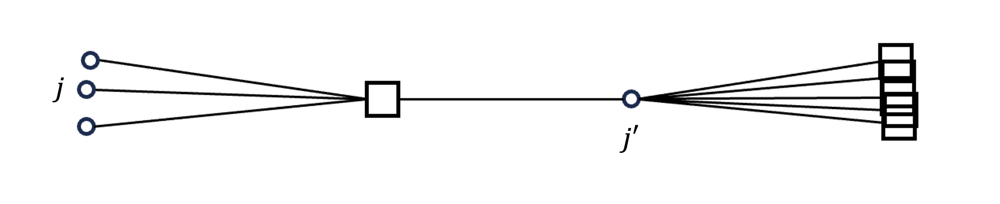
It turns out that the instance around must exhibit a very specific structure in order to ensure that the 3-hop triangle inequality is tight for almost every neighbor . We must have almost every located around almost the same point at distance from , where almost all facility neighbors of are at the opposite end of the line connecting and . See Figure 1 for an example. Intuitively, the existence of such a dense region of clients suggests that if we let a client in the region as a new center, many of the 3-hop-triangle inequalities cannot be tight, which implies average rerouting cost . If is again problematic, we can repeat this procedure over and over.
However, if we relax the condition to , certain exceptions begin to emerge. One possible scenario is as follows: Since captures the rerouting of to ’s close facilities except the ’s facilities , if is large enough to exclude the facilities of , then might not behave as expected. However, a large volume of implies low ratio. If the ratio is sufficiently low, then this facility-dominant instance is actually easier to handle with a completely different algorithm, the JMS algorithm [12], which is known to be -approximation algorithm.
Therefore, from now on, assume that the cluster centered at is connection-dominant. More strictly, assume that for any neighbor of cluster center satisfies that cannot cover half of the ball centered at with a radius of . At this point, we can finally assert that it is impossible to avoid the formation of a dense region of clients.
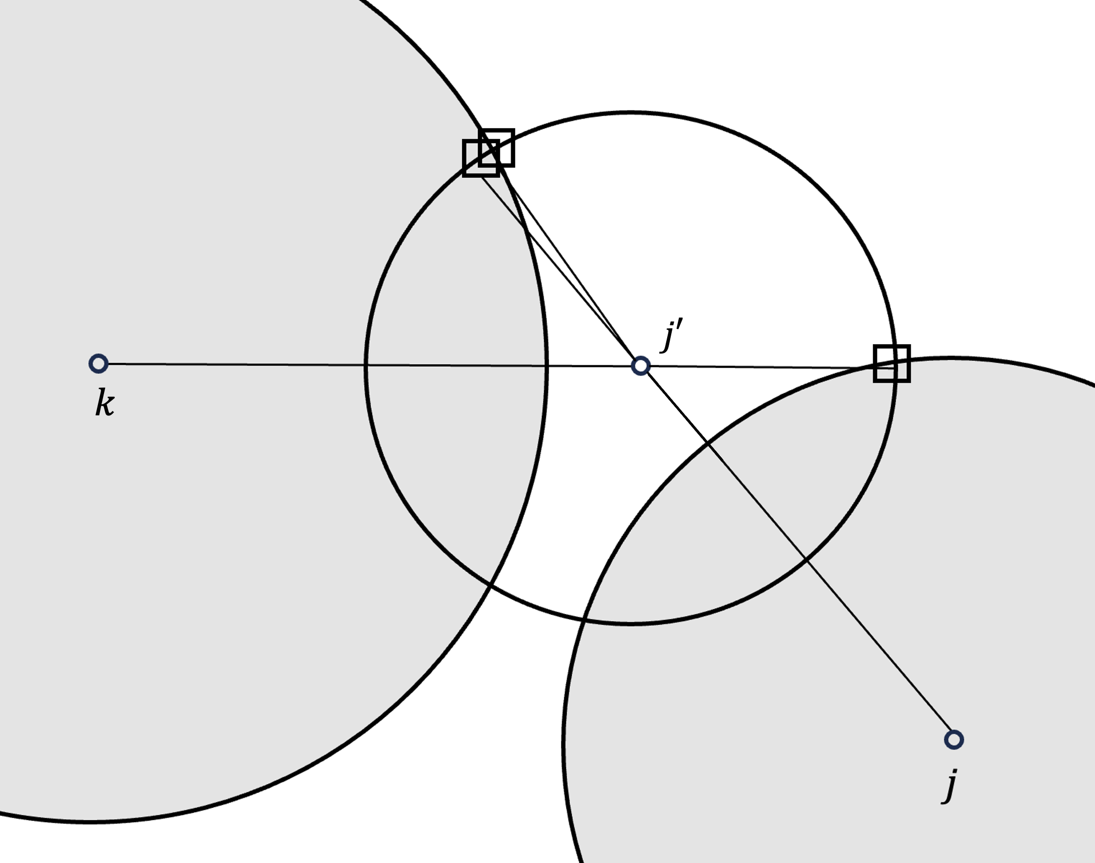
Assume towards contradiction that there is no dense region and consider in ’s cluster such that . Almost all facilities of must be placed in one of two locations: on the opposite side of relative to , or within . Since there is no dense region, there must be a neighbor of such that , and is located in a different direction from . This implies that the facilities positioned on the opposite side of now help reduce , forcing that they are in ; since we assumed that cannot cover half of the unit ball around , it implies the angle must be strictly greater than ! Ultimately, this process can be simplified to the following situation: inserting unit vectors into a unit sphere with every pairwise angle greater than for some constant . It is well known that in the geometry of Euclidean space, there is an upper bound on the number of such vectors, and such an upper bound shows that one of the regions around (or ) we considered must have been dense. See Figure 2 for an example.
However, there are several technical barriers to extending this notion to the general case without restrictions on , , and . In Section 3, we introduce these barriers and formalize the above concept. We also propose sufficient conditions to satisfy (1). From Section 3.1 to Section 5, we demonstrate how to remove these conditions, leaving only the connection-dominant instance assumptions. In Section 6, we propose and analyze the full algorithm, which achieves improved bi-factor approximation performance.
3 Finding Good Center via Geometry
In this section, we exploit the geometry of Euclidean spaces to prove the existence of a cluster center strictly better than the greedy choice of [3] under certain conditions (Theorem 10). We first define several concepts and introduce their motivation, including the sketch of our algorithm.
Recall that our goal is to find a cluster that satisfies (1). In all the following propositions, is a fixed value in the range .
Definition 4.
Suppose is a cluster center. Let be the set of neighbors of , and . Additionally, define two more sets:
Moreover, Saving and Spending of center is defined as
With the goal (1) in mind, (resp. ) contains clients who meet (resp. do not meet) this goal, and (resp. ) indicates how much exceeds (resp. is short of) this goal. Note that by definition; it is the best cluster for center , which contains all its neighbors (which is required by the algorithm design) and possibly more to increase savings. Therefore, if , then is considered a good center; otherwise, it is a bad center.
Now, we will explain some problematic situations that arise when extending the problem to the general case, i.e., without restrictions on , , and ’s. The first simple concern is that the choice of the center will no longer be solely based on as in Algorithm 1, which breaks the previous arguments. Therefore, to gain more flexibility in selecting a new cluster center, it is beneficial to decompose the entire support graph into several layers, where each layer only concerns clients with roughly the same values.
Definition 5.
A network is a subgraph of the support graph . A network is called homogeneous if there exists , such that for any client , for .
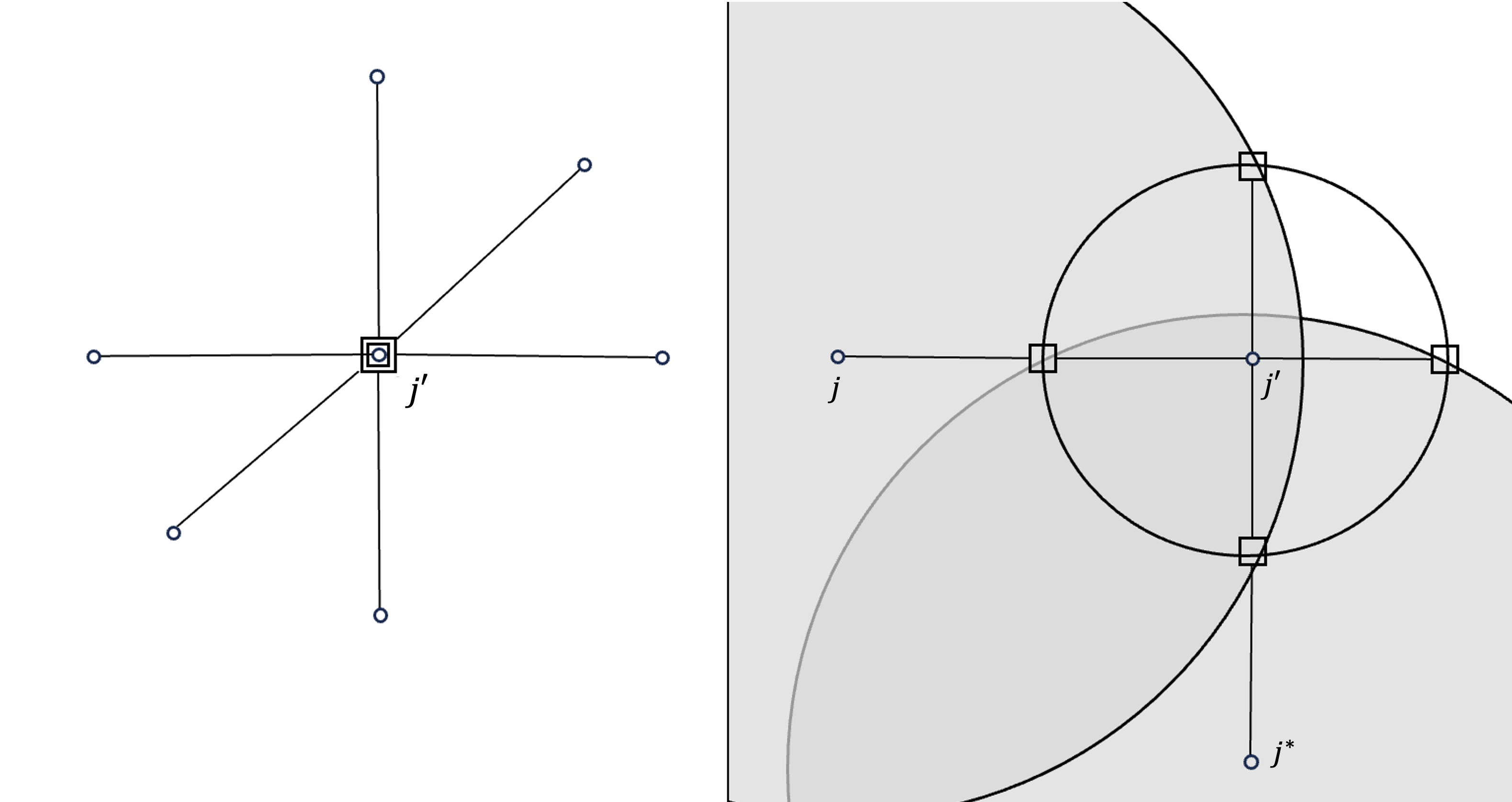
However, there are still two more scenarios where the above strategy might not hold, as illustrated in Figure 3. This means that the neighbors in are all bad clients, but do not create a dense region.
-
I.
If , the facilities in are concentrated near . In this case, since all the facilities are very close to , the 3-hop triangle inequality is almost tight for any regardless of where it is.
-
II.
Recall that if is large enough to exclude the facilities of , then might not behave as expected. In particular, a technical problem arises when two facilities from that are almost antipodal with respect to are both contained in , which is illustrated in Figure 3 (right).
The following definition addresses Scenario I.
Definition 6.
For , let . A client is normal if , otherwise weird.
The following definition addresses Scenario II. Note that is the maximum distance between and any facility in . We are interested in the ball around of radius (for sake of analysis), and having a small remote arm with respect to means that cannot contain two antipodal points in our ball of interest (with some slack depending on ). Let . The right-hand side represents the square of the length of the other side of a triangle, where the lengths of the two sides are and , and the included angle between them is .
Definition 7.
For normal center , a neighbor of is said to have a small remote arm if the following holds for .
Otherwise, is said to have a big remote arm.
In Section 3.1, we will show that these two scenarios are the only bad cases to worry about. For instance, if we assume that everything is normal and has a small remote arm, each candidate center is either good or contains another candidate center with in its dense region.
How can we handle these two bad scenarios? In the following two lemmas, we prove that both the weird center and the big remote arm neighbor imply a high ratio of fractional facility cost to fractional connection cost . The proof appears in the extended version of this paper [14].
Lemma 8.
For any weird client , holds.
Lemma 9.
When , for a normal center , if has a big remote arm, then .
Therefore, if we consider a (sub)instance that has a low facility-to-connection cost ratio, it is natural to expect to apply this argument, which ultimately leads to a (somewhat) good center. Throughout the paper, we will often express this low facility-to-connection ratio condition will be expressed as and use the following values for : . The following theorem is the main result of the section.
Theorem 10.
Consider a homogeneous network and let be the normal center with the highest saving among all normal centers. Let and . If , then this cluster is good on average for and every . i.e.
3.1 Geometric Arguments
In this subsection, we prove Theorem 10 using properties of Euclidean geometry. As previously discussed, our goal is to show: When a bad cluster center is normal and (many of) its neighbors have a small remote arm, it is possible to find a dense region of clients near .
When we consider the rerouting of to ’s close facilities , we can define some worst facilities. In the below definition, is the set of facilities that have the (almost) worst distance from , and is the set of facilities with both worst distance and worst angle.
Definition 11.
Let , and let be the minimum angle that satisfies for . For and its center , let
The following lemma shows that if is normal and has a bad rerouting through , then among the facilities in , which are the rerouting candidates with worst distance, more than half of them must have a bad angle as well. It is a formalization of the intuition illustrated in Figure 1.
Lemma 12.
For any of normal center , .
Proof.
By the triangle inequality and the homogeneous condition,
Lemma 13.
For a normal center and any , let , . Then the following holds:
Proof.
Assume the nontrivial case: . Let . Let rerouting probability and rerouting length for as:
Note that and . Then the goal of this theorem can be written as .
By Lemma 12, holds. We derive a lower bound for as:
implies that
since the right-hand side gives the minimum value when is the maximum. It is bounded because is normal.
Denote a position vector as . From the definition of , is at most
Therefore, since , holds. It implies
From the homogeneous condition,
which implies
The following argument demonstrates how the positional distribution of facilities in restricts that of the neighbors in . Consider two neighbors , both with small remote arms, separated by an angle greater than , say . Then, . However, facilities in reduce and vice versa, which implies that either or vice versa. As the small remote arm condition of puts a limit on how much can intersect , it is natural to expect that the number of such pairs is small.
Theorem 14.
For a normal center , let be a subset of , consisting of clients with a small remote arm. Furthermore, let any two elements be separated by an angle greater than with respect to center , i.e., . Then, the cardinality of is bounded by , independent of the Euclidean space’s dimension.
Proof.
Denote . Without loss of generality,
for all . Suppose for some . Additionally, given and the small arm condition, it implies . Therefore, . Moreover, since . However, it contradicts to Lemma 13.
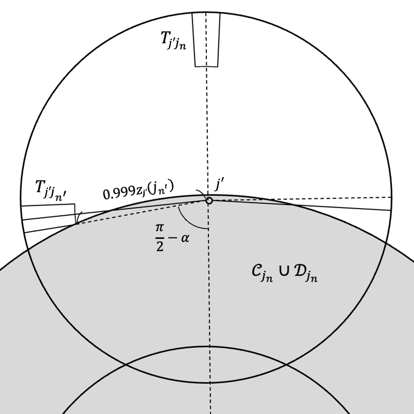
We show that two ’s in with similar values form a large angle with . Suppose for some with . Then for any point , it holds that and . Also, the quadratic function is shown to be non-decreasing for . It comes from Lemma 12, which ensures that . Therefore, since has a small remote arm,
which implies , contradicting to the above result. Refer to Figure 4.
According to Rankin [17], the maximum number of disjoint spherical caps, each with an angular radius of , is at most in any dimension. Since holds, it is feasible to segment this range into successive subranges such as , , …, up to . Thus each subrange can only contain a finite number of clients with a small remote arm. Moreover, the normal center condition ensures a bounded number of such divisions. Consequently, the cardinality of is at most
Therefore, if we have a large with small remote arms, there must exist a large subset of whose pairwise angle is small, creating a dense region.
Lemma 15.
For a normal center , let be a set of clients from with a small remote arm. If , then there exists a client for which .
Proof.
Let be a maximal subset of where any two clients are separated by an angle greater than with respect to the center . Then, for any client , there exists a client such that . Therefore, there exists a such that the number of clients for which is at least .
For , let be a region where
Therefore, there exists an index such that . For any two clients , the distance is bounded by the sum of their radial and angular differences. Hence, . From the triangle inequality and the homogeneous condition,
which implies . By Theorem 14, . Therefore, the saving of any client is at least
Given these geometric tools, Theorem 10 follows as the number of big-remote-arm-neighbors of the chosen center can be bounded.
4 Clustering for Homogeneous Instances
In this section, we present an algorithm that operates on a connection-dominant homogeneous instance, ensuring strictly better performance than a naive greedy clustering strategy. Let for be the center of when some clustering is given in the context.
Theorem 16.
Suppose a homogeneous network satisfies . Then, the clustering produced by Algorithm 2 is good on average. Precisely, for and every , the following holds:
For one of a cluster made by the algorithm, if the center of is weird, then the ratio is at most since all clients within them are weird. If is not “good”, its connection-facility ratio is at most by Theorem 10. Therefore, the assumed ratio in this theorem is larger than these values, implying that a constant proportion of clusters are “good” since they satisfy the conditions of Theorem 10. Therefore, by reducing the value by that proportion, the desired result can be obtained.
Proof.
Divide into three groups:
-
1.
Clients clustered by a normal center, where the ratio of that cluster’s connection cost to facility cost is greater than .
-
2.
Clients clustered by a normal center, where this ratio is at most .
-
3.
Clients clustered by a weird center.
Let be the set of clients in the -th group (. Here, and correspond to clusters formed by the if condition, and is formed by the else condition. Define the following values:
By Theorem 10, . The rerouting cost for is only bounded by the homogeneous condition. For a client , . Lastly, clients in are clustered through a greedy strategy. Thus, . Note that consists solely of weird clients, meaning .
From above, the total rerouting cost is bounded by:
Therefore, it is sufficient to show that
Note that holds, which means . Also , since . Then the following holds:
5 Clustering for Connection-dominant Instances
In this section, we introduce an algorithm that operates on connection-dominant instances without a homogeneous condition. This algorithm uses Algorithm 1 and Algorithm 2 as subroutines. The theorem stated below shows our main result.
Theorem 17.
For any connection-dominant instance, i.e. , there exists an algorithm that finds a clustering configuration whose rerouting cost is at most
for and every .
Definition 18.
Let be the set of clients for which . Let . For , let a Block be the set of clients such that
Note that if , then a network composed of at most consecutive blocks is still homogeneous. However, applying Algorithm 2 directly to each block would be impossible when the block is a facility-dominant or neighbors of the center from some block may belong to a different block. Moreover, the following fact implies that the neighbor relationships between consecutive blocks are the main point.
Observation 19.
If two neighbors belonging to neither the same block nor consecutive blocks, satisfying , then holds when criteria satisfies that .
Proof.
A key idea is that with a sufficiently small , the support graph can be segmented almost arbitrarily while still preserving the homogeneous condition, enabling the identification of weak connections between consecutive blocks. Notably, even if two clients and come from consecutive blocks, the is not worse than the greedy strategy.
Definition 20.
An interval is the set of consecutive blocks, up to a maximum for . Precisely, for , where , except when . The size of an interval is the number of blocks it contains, denoted as . The reward of interval is defined as .
Note that a block is a unique type of interval with a size of . Also holds. An interval is the basic unit of clustering to which Algorithm 1 and Algorithm 2 are applied. Therefore, the reward of an interval represents the extent to which a guaranteed can be obtained when the current interval can be clustered using Algorithm 2, regardless of how the preceding intervals have been clustered. From this perspective, the first block, which does not contribute to the reward, serves as a kind of “buffer”.
Given the entire support graph and a subset , let be the subgraph (network) induced by . Consequently, when we call Algorithms 1 or 2 with , the calculations for and are performed solely with respect to the implicitly defined client set . We denote Algorithm 1 as greedy and Algorithm 2 as homogeneous. For simplicity, when denotes an interval, we interpret the expression as , aggregating over all clients within the interval. The following theorem illustrates how reward is related to . The proof appears in the extended version of this paper [14].
Lemma 21.
Let be a set of non-overlapping intervals. Then clustering produced by Algorithm 3 is good on average. Precisely, for ,
In conclusion, it suffices to find a set of non-overlapping intervals which have a high value. Here, we will briefly touch on the idea. We will iterate through the blocks in reverse order , cutting out suitable ranges that satisfy the interval conditions. Fix a point to be the right end of the interval, and expand the left end of the current range one block to the left until the range is suitable for processing. Suppose, at some point, the value of the current range is less than , which is strictly less ratio of the input instance, . Then, this range can be considered a minor part and can be excluded as there is no need for it to become an interval. Therefore, we only consider cases where the current range has a value of at least .
However, in the situation where the current range’s reward is small, meaning that the first block must avoid most of the . In this case, if we keep expanding the range to the left, we will eventually reach the initial block , satisfying the interval condition. There remains a subtle issue of the range’s length exceeding during the expansion process, but this implies that the value on the left side of the range is always exponentially increasing compared to the right side. This can be resolved by appropriately reducing the right side of the range.
Lemma 22.
For any support graph that is connection-dominant, , then the set of non-overlapping intervals obtained by Algorithm 4 satisfies .
The proof appears in the extended version of this paper [14].
6 Improved Bifactor Approximation
7 Improved Unifactor Approximation
In this section, we propose the algorithm that guarantees better unifactor approximation suggested by Li [15], proving Theorem 2.
Framework of [15].
Li showed that a hard instance for a certain might not be a hard instance for another value of . This suggests that selecting a value at random could improve the expected performance of the algorithm.
They introduced a characteristic function to represent the distribution of distances between a client and its neighboring facilities. For a client , assume are the facilities within , ordered by increasing distance from . Then, for , is defined as , where is the smallest index satisfying . Also, they improved the bound of the rerouting cost as . For fixed , the expected connection cost for for the aforementioned algorithm of [3] is at most
Therefore, it can be modeled as a -sum game to analyze the approximation ratio. The characteristic function for the whole instance is given by . Assuming is normalized so that , the algorithm proceeds as follows: with probability , it employs the JMS algorithm [12]. Mahdian [16] proved that the JMS algorithm achieves a -approximation. Otherwise, is sampled randomly from the distribution , ensuring that . Thus, the value of the -sum game, i.e., the approximation ratio of the algorithm under a fixed strategy , is calculated as follows:
where
Moreover, for a given probability density function for , it can be shown that the characteristic function for the hardest instance is a threshold function, which defined as
for some . This means that the final approximation ratio for some is given by . In [15], the suggested distribution for is , where is Dirac delta function, , , , .
Our Improvement.
By using Algorithm 5, the expected connection cost for some and characteristic function is given as follows:
Therefore, we define a new -sum game value as follows, assuming is scaled up such that .
Note that is still linear for . Therefore, even if the game definition changes, the adversary’s choice of the characteristic function remains a threshold function for some . Given that there is a positive probability of sampling between and , it is possible to achieve a lower cost.
Lemma 23.
Let , where is a Dirac-delta function. Then the following holds:
The proof appears in the extended version of this paper [14].
Therefore, we present an improved unifactor approximation algorithm, Algorithm 6.
8 APX-Hardness
In this section, we prove that UFL is APX-Hard in Euclidean spaces. We use the following result from Austrin, Khot, and Safra [2]. For and , let where are standard Gaussian random variables with covariance and is the cumulative density function of the standard normal distribution.
Theorem 24.
Assuming the Unique Games Conjecture, for any and , it is NP-hard to, given a graph , distinguish between the following two cases.
-
(Completeness) contains an independent set of size .
-
(Soundness) For any , the number of edges with both endpoints in is at least where .
Fix an arbitrary . Without loss of generality, assume . Also let . Our UFL instance has as the set of facilities and as the set of clients. The ambient Euclidean space is , and let be the th standard unit vector (i.e., and for every ). Then each facility is located at and each client is located at . Finally, let be the common facility cost for every to be determined. This finishes the description of the UFL instance.
In the completeness case, there is an independent set of size . We open . Since is a vertex cover, every client in has a facility at distance , so the total cost is
In the soundness case, consider any solution that opens and let and . By the soundness guarantee, at least clients do not have a facility at distance . Since every client-facility distance is either or , the total cost is at least
| (2) |
For fixed , the function is a strictly convex function of , so if we let such that
then (2) is minimized when when , which becomes
Furthermore, we can notice that
Then one can see that the optimal value in the soundness case is at least larger than the optimal value in the completeness case. For a fixed , by choosing sufficiently small, one can ensure that this excess is at least a fraction of the completeness case optimal value for some constant , which proves a -hardness of approximation.
9 Conclusion
The most natural open problem is to get an improved approximation for bifactor or unifactor approximation for UFL. Though we show a strict separation between general and Euclidean metrics for bifactor approximation in a certain regime, it is not achieved for all regimes of bifactor or unifactor approximation.
Whereas our algorithm is based on the primal rounding approach of [3] and [15], it might be a fruitful research direction to design a variant of the Jain-Mahdian-Saberi algorithm [12] (greedy algorithm analyzed by the dual fitting method) or Jain-Vazirani [13] (primal-dual algorithm) for a further improvement. In particular, as the best unifactor approximation for UFL in both general and Euclidean metrics employ the -approximation of the JMS algorithm as a black box, improving the JMS algorithm will directly yield a better result for the best unifactor approximation for UFL. The JV algorithm was already improved in Euclidean spaces [1, 10, 4], but they are not enough for UFL.
References
- [1] Sara Ahmadian, Ashkan Norouzi-Fard, Ola Svensson, and Justin Ward. Better guarantees for k-means and euclidean k-median by primal-dual algorithms. SIAM Journal on Computing, 49(4):FOCS17–97, 2019. doi:10.1137/18M1171321.
- [2] Per Austrin, Subhash Khot, and Muli Safra. Inapproximability of vertex cover and independent set in bounded degree graphs. Theory of Computing, 7(1):27–43, 2011. doi:10.4086/TOC.2011.V007A003.
- [3] Jaroslaw Byrka and Karen Aardal. An optimal bifactor approximation algorithm for the metric uncapacitated facility location problem. SIAM Journal on Computing, 39(6):2212–2231, 2010. doi:10.1137/070708901.
- [4] Vincent Cohen-Addad, Hossein Esfandiari, Vahab Mirrokni, and Shyam Narayanan. Improved approximations for euclidean k-means and k-median, via nested quasi-independent sets. In Proceedings of the 54th Annual ACM SIGACT Symposium on Theory of Computing, pages 1621–1628, 2022. doi:10.1145/3519935.3520011.
- [5] Vincent Cohen-Addad, Andreas Emil Feldmann, and David Saulpic. Near-linear time approximation schemes for clustering in doubling metrics. Journal of the ACM (JACM), 68(6):1–34, 2021. doi:10.1145/3477541.
- [6] Vincent Cohen-Addad and CS Karthik. Inapproximability of clustering in lp metrics. In 2019 IEEE 60th Annual Symposium on Foundations of Computer Science (FOCS), pages 519–539. IEEE, 2019.
- [7] Vincent Cohen-Addad, Karthik C S, and Euiwoong Lee. Johnson coverage hypothesis: Inapproximability of k-means and k-median in -metrics. In Proceedings of the 2022 Annual ACM-SIAM Symposium on Discrete Algorithms (SODA), pages 1493–1530. SIAM, 2022. doi:10.1137/1.9781611977073.63.
- [8] Vincent Cohen-Addad Viallat, Fabrizio Grandoni, Euiwoong Lee, and Chris Schwiegelshohn. Breaching the 2 lmp approximation barrier for facility location with applications to k-median. In Proceedings of the 2023 Annual ACM-SIAM Symposium on Discrete Algorithms (SODA), pages 940–986. SIAM, 2023.
- [9] Kishen N Gowda, Thomas Pensyl, Aravind Srinivasan, and Khoa Trinh. Improved bi-point rounding algorithms and a golden barrier for k-median. In Proceedings of the 2023 Annual ACM-SIAM Symposium on Discrete Algorithms (SODA), pages 987–1011. SIAM, 2023. doi:10.1137/1.9781611977554.CH38.
- [10] Fabrizio Grandoni, Rafail Ostrovsky, Yuval Rabani, Leonard J Schulman, and Rakesh Venkat. A refined approximation for euclidean k-means. Information Processing Letters, 176:106251, 2022. doi:10.1016/J.IPL.2022.106251.
- [11] Sudipto Guha and Samir Khuller. Greedy strikes back: Improved facility location algorithms. Journal of algorithms, 31(1):228–248, 1999. doi:10.1006/JAGM.1998.0993.
- [12] Kamal Jain, Mohammad Mahdian, and Amin Saberi. A new greedy approach for facility location problems. In Proceedings of the thiry-fourth annual ACM symposium on Theory of computing, pages 731–740, 2002. doi:10.1145/509907.510012.
- [13] Kamal Jain and Vijay V Vazirani. Approximation algorithms for metric facility location and k-median problems using the primal-dual schema and lagrangian relaxation. Journal of the ACM (JACM), 48(2):274–296, 2001. doi:10.1145/375827.375845.
- [14] Euiwoong Lee and Kijun Shin. Facility location on high-dimensional euclidean spaces, 2024. arXiv:2501.18105.
- [15] Shi Li. A 1.488 approximation algorithm for the uncapacitated facility location problem. Information and Computation, 222:45–58, 2013. doi:10.1016/J.IC.2012.01.007.
- [16] Mohammad Mahdian, Yinyu Ye, and Jiawei Zhang. A 1.52-approximation algorithm for the uncapacitated facility location problem. In Proc. of APPROX, pages 229–242, 2002.
- [17] Robert Alexander Rankin. The closest packing of spherical caps in n dimensions. Glasgow Mathematical Journal, 2(3):139–144, 1955.