Being Efficient in Time, Space, and Workload:
a Self-Stabilizing Unison and Its Consequences

Self-stabilization is a general non-masking and lightweight fault tolerance paradigm [25, 3]. Precisely, a distributed system achieving this property inherently tolerates any finite number of transient faults.¹¹1A transient fault occurs at an unpredictable time, but does not result in a permanent hardware damage. Moreover, as opposed to intermittent faults, the frequency of transient faults is considered to be low. Indeed, starting from an arbitrary configuration, which may be the result of such faults, a self-stabilizing system recovers within finite time, and without any external intervention, a so-called legitimate configuration from which it satisfies its specification.

In this paper, we consider the most commonly used model in the self-stabilizing area: the atomic-state model [25, 3]. In this model, the state of each node is stored into registers and these registers can be directly read by neighboring nodes. Furthermore, in one atomic step, a node can read its state and that of its neighbors, perform some local computation, and update its state accordingly. In the atomic-state model, asynchrony is materialized by an adversary called daemon that can restrict the set of possible executions. We consider here the weakest (i.e., the most general) daemon: the distributed unfair daemon.

Self-stabilizing algorithms are mainly compared according to their stabilization time, i.e., the worst-case time to reach a legitimate configuration starting from an arbitrary one. In the atomic-state model, stabilization time can be evaluated in terms of rounds and moves. Rounds [13] capture the execution time according to the speed of the slowest nodes. Moves count the number of local state updates. So, the move complexity is rather a measure of work than a measure of time. It turns out that obtaining efficient stabilization times both in rounds and moves is a difficult task. Usually, techniques to design an algorithm achieving a stabilization time polynomial in moves make its round complexity inherently linear in $n$, the number of nodes (see, e.g., [2, 23, 19]). Conversely, achieving the asymptotic optimality in rounds, usually $O(D)$ where $D$ is the network diameter, commonly makes the stabilization time exponential in moves (see, e.g., [22, 31]). Surprisingly, Cournier, Rovedakis, and Villain [14] manage to prove the first fully polynomial (i.e., with $Poly(n)$ move and $Poly(D)$ round complexities) silent²²2In the atomic-state model, a self-stabilizing algorithm is silent if all its executions terminate. self-stabilizing algorithm. Their algorithm builds a BFS (Breadth-First Search) spanning tree in any rooted connected network and they prove that it stabilizes in $O(n^6)$ moves and $O(D^2)$ rounds using $\mathrm{\Theta }(\log B+\log \mathrm{\Delta })$ bits per node, where $B$ is an upper bound on $D$ and $\mathrm{\Delta }$ is the maximum degree of the network.

Up to now, fully polynomial self-stabilizing algorithms have only been proposed (see [14, 21]) for so called static problems [34], such as spanning tree constructions and leader election, which compute a fixed object in finite time. In this paper, we propose an algorithm for a fundamental dynamic (i.e., non static) problem: the asynchronous unison (unison for short). It consists in maintaining a local clock at each node. The domain of clocks can be bounded (like everyday clocks) or infinite. The liveness property of the problem requests each node to increment its own clock infinitely often. Furthermore, the safety property of the unison requires the difference between the clocks of any two neighbors to always be at most one increment. The usefulness of the unison comes from the fact that asynchrony often makes fault tolerance very difficult in distributed systems. The impossibility of achieving consensus in an asynchronous system in spite of at most one process crash [30] is a famous example illustrating this fact. Thus, fault tolerance, and in particular self-stabilization, often requires some kind of barrier synchronization, which the unison provides, to control the asynchronism of the system by making processes progress roughly at the same speed. Unison is thus a fundamental algorithmic tool that has numerous applications. Among others, it can be used to simulate synchronous systems in asynchronous environments [17], to free an asynchronous system from its fairness assumption (e.g., using the cross-over composition) [8], to facilitate the termination detection [9], to locally share resources [11], or to achieve infimum computations [10]. Thus, as expected, we also derive from our unison algorithm a synchronizer allowing us to obtain several new state-of-the-art self-stabilizing algorithms for various problems, including spanning tree problems and leader election.

The rest of the paper is organized as follows. Section 2 is dedicated to the computational model and the basic definitions. We develop the links between the present paper and [21] in Section 3, and we present our algorithm in Section 4. We sketch its correctness and its time complexity in Section 5. In Section 6, the self-stabilizing synchronizer derived from our unison algorithm is presented and its complexity is also sketched. We conclude in Section 7.

We model distributed systems as simple graphs, that is, pairs $G=(V,E)$ where $V$ is a set of nodes and $E$ is a set of edges representing communication links. We assume that communications are bidirectional. The set $N(p)=\{q\mid \{p,q\}\in E\}$ is the set of neighbors of $p$, with which $p$ can communicate, and $N[p]=N(p)\cup \{p\}$ is the closed neighborhood of $p$. A path (from $p_0$ to $p_l$) of length $l$ is a sequence $P=p_0{p}_1\mathrm{\cdots }{p}_l$ of nodes such that consecutive nodes in $P$ are neighbors. We assume that $G$ is connected, meaning that any two nodes are connected by a path. We can thus define the distance $d(p,q)$ between two nodes $p$ and $q$ to be the minimum length of a path from $p$ to $q$. The diameter $D$ of $G$ is then the maximum distance between nodes of $G$.

Our unison algorithm works in a variant of the atomic-state model in which each node holds locally shared registers, called variables, whose values constitute its state. The vector of all node states defines a configuration of the system.

An algorithm consists of a finite set of rules of the form $label:guard\to action$. In the variant that we consider, a guard is a boolean predicate on the state of the node and on the set of states of its neighbors. The action changes the state of the node. To shorten guards and increase readability, priorities between rules may be set. A rule whose guard is true is enabled, and can be executed. By extension, a node with at least one enabled rule is also enabled, and $Enabled(\gamma )$ contains the enabled nodes in a configuration $\gamma$. Note that this model is quite weak. Indeed, in other variants, nodes may have, for example, distinct identifiers. In our case, the network is anonymous and since a node only accesses a set of states, it cannot even count how many neighbors it has.

An execution in this model is a maximal sequence of configurations $e={\gamma }^0{\gamma }^1\mathrm{\cdots }{\gamma }^i\mathrm{\cdots }$ such that for each transition (called step) ${\gamma }^i\mapsto {\gamma }^{i+1}$, there is a nonempty subset ${𝒳}^i$ of $Enabled({\gamma }^i)$ whose nodes simultaneously and atomically execute one of their enabled rules, leading from ${\gamma }^i$ to ${\gamma }^{i+1}$. We say that each node of ${𝒳}^i$ executes a move during ${\gamma }^i\mapsto {\gamma }^{i+1}$. Note that $e$ is either infinite, or ends at a terminal configuration ${\gamma }^f$ where $Enabled({\gamma }^f)=\mathrm{\varnothing }$. An algorithm with no infinite executions is terminating or silent.

A daemon $𝔇$ is a predicate over executions. An execution which satisfies $𝔇$ is said to be an execution under $𝔇$. We consider the synchronous daemon, which is true if, at all steps, ${𝒳}^i:=Enabled({\gamma }^i)$, and the fully asynchronous daemon, also called distributed unfair daemon in the literature, which is always true. Note that under the distributed unfair daemon, a node may starve and may never be activated, unless it is the only enabled node.

In an execution, all the information in the states is not necessarily relevant for a problem. We thus use a projection to extract information (e.g., just an output boolean for the boolean consensus) from a node’s state, and we canonically extend this projection to configurations and executions. A specification of a distributed problem is then a predicate over projected executions. A problem is static if its specification requires the projected executions to be constant, and it is dynamic otherwise.

An algorithm is self-stabilizing under a daemon $𝔇$ if, for every network and input parameters, there exists a set of legitimate configurations such that (1) the algorithm converges, i.e., every execution under $𝔇$ (starting from an arbitrary configuration) contains a legitimate configuration, and (2) the algorithm is correct, i.e., every execution under $𝔇$ that starts from a legitimate configuration satisfies the specification.

We consider three complexity measures: space, moves which model the total workload, and rounds which model an analogous of the synchronous time by taking the speed of the slowest nodes into account. As done in the literature on the atomic-state model, the space complexity is the maximum space used by one node to store its own variables. As explained before, a move is the execution of a rule by a node. To define the round complexity of an execution $e={\gamma }^0{\gamma }^1\mathrm{\cdots }$, we first need to define the notion of neutralization: a node $p$ is neutralized in ${\gamma }^i\mapsto {\gamma }^{i+1}$, if $p$ is enabled in ${\gamma }^i$ and not in ${\gamma }^{i+1}$, but it does not apply any rule in ${\gamma }^i\mapsto {\gamma }^{i+1}$. Then, the rounds are inductively defined as follows. The first round of an execution $e={\gamma }^0{\gamma }^1\mathrm{\cdots }$ is the minimal prefix $e^{\prime }$ such that every node that is enabled in ${\gamma }^0$ either executes a move or is neutralized during a step of $e^{\prime }$. If $e^{\prime }$ is finite, then let $e^{\prime \prime }$ be the suffix of $e$ that starts from the last configuration of $e^{\prime }$; the second round of $e$ is the first round of $e^{\prime \prime }$, and so on. For every $i>0$, we denote by ${\gamma }^{r_i}$ the last configuration of the $i$-th round of $e$, if it exists and is finite; we also conventionally let ${\gamma }^{r_0}={\gamma }^0$. Consequently, ${\gamma }^{r_{i-1}}$ is also the first configuration of the $i$-th round of $e$. The stabilization time of a self-stabilizing algorithm is the maximum time (in moves or rounds) over every execution possible under the considered daemon (starting from any initial configuration) to reach (for the first time) a legitimate configuration.

We started this work on the bounded unison problem when we observed that an unbounded solution can easily be derived from [21]. This can be seen as follows. The algorithm given in [21] simulates a synchronous non self-stabilizing algorithm in an asynchronous self-stabilizing setting. To do so, it uses a very natural idea. It stores, at each node, the whole execution of the algorithm so far as a list of states. Given its list and the lists of its neighbors, a given node can check for inconsistencies in the simulation and correct them.

Now if we implement this idea in an asynchronous algorithm which is not self-stabilizing, then the length of the lists satisfy the unison property. Indeed, to compute its $(i+1)$-th value, a node must wait for all its neighbors to have computed at least their $i$-th value.

Obviously, in a self-stabilizing setting, we cannot expect the length of the lists of the nodes to initially satisfy the unison property. It turns out that the error recovery mechanism in [21] not only solves the initial inconsistencies of the simulation, but also recovers the unison property.

If we simulate an algorithm “that does nothing”, we can compress the lists by only storing their lengths. We thus obtain a first (unbounded) unison algorithm, given below. Note that although we describe the whole algorithm, the reader does not need to fully understand it.

Each node $p$ has a status $p.s\in \{E,C\}$ (Error/Correct) and a time $p.t\in \mathbb{N}$. Given these predicates,

the algorithm is defined by the following four rules

in which $R_R$ has the highest priority, and $R_P(i)$ has a higher priority than $R_P(i^{\prime })$ for . The rules $R_R$, $R_P(i)$ and $R_C$ are “error management” rules. Thus, once the algorithm has stabilized, the status of all nodes is $C$ and only $R_U$ is applicable.

This unbounded self-stabilizing unison algorithm is not really interesting by itself. Indeed, it converges in $2D+2$ rounds in an asynchronous setting, but in this regard, the algorithm in [4] converges twice as fast, is simpler and operates in the message-passing model, which is more realistic. However, whereas nobody has been able to derive a bounded version of the algorithm in [4], we hoped that this could be done with this new algorithm.

In the following subsections, we present a first very natural attempt, which ultimately failed, and a more complex version, which we detail and prove in the next sections of the paper.

The most natural strategy to turn an unbounded unison into a bounded one is simply to count modulo a large enough fixed bound $B$. To outline this change of paradigm from an ever-increasing time to a circular clock, we rename the variable $p.t$ into $p.c$ for any node $p$. We thus modify the rule $R_U$ as follows:

At first glance, we do not need to modify the other rules as their purpose is only to correct errors, but this intuition is wrong. Indeed, when two neighboring nodes $p$ and $q$ are such that $p.s=q.s=C$, $p.c=0$ and $q.c=B-1$, they satisfy the unison property, but $p$ can apply the rule $R_R$, although there are no errors to correct. The problem comes from the term $\exists q\in N(p),(q.c\ge p.c+2)$ in the $root$ predicate which should detect out-of-sync neighbors. Hence, we must at least modify this predicate as follows:

Therefore, transforming the algorithm to implement this simple modulo-$B$ idea is already not as straightforward as it may seem.

Moreover, even small modifications generally introduce new unforeseen behaviors, and the modified algorithm has no particular reasons to be efficient, or even correct. As a matter of fact, we failed to prove its correctness. To understand why, we must delve a bit into the proof scheme of [21].

An important observation is that rootless configurations (i.e., those without nodes satisfying the $root$ predicate) satisfy the safety property of the unison. In [21], the correctness and the move complexity then follow from the key property that roots cannot be created, and that, in a “small” number of steps, at least one root disappears.

Sadly, this first attempt algorithm does not satisfy the “no root creations” property. To see this, consider a path $p-q-r$ and a configuration ${\gamma }^a$ in which $p.c=q.c=B-1$, $r.c=3$, $p.s=q.s=C$ and $r.s=E$. In one step ${\gamma }^a\mapsto {\gamma }^b$,

• $\mathrm{■}$

  $p$ applies the rule $R_U$ and thus, in ${\gamma }^b$, $p.c=0$ and $p.s=C$

• $\mathrm{■}$

  $q$ applies the rule $R_P(4)$, and thus, in ${\gamma }^b$, $q.c=4$.

Therefore, in ${\gamma }^b$, $p.s=C$ and $p$ has a neighbor $q$ such that $q.c\ge p.c+2$ and $q.c\ne B-1$. Thus, $p$ is a root in ${\gamma }^b$, although it is not one in ${\gamma }^a$.

Note that the fact that roots can be created is not necessarily a problem. Indeed, if only a finite number of them appears, we recover the correctness of the algorithm. We actually believe that, for $B$ large enough, any node can become a root only once per execution, and this would most likely imply that the move complexity remains polynomial. But $n$ roots may appear sequentially, which would lead to an $\mathrm{\Omega }(n)$ round complexity.

At this point, we cannot rule out that this algorithm is correct and has good properties. However, because of these problems, we took another approach.

In the end, our solution is obtained by a rather limited modification of the previous algorithm: we extend the range of the counters $p.c$ to the interval $[-B,B)$, but we restrict their range to $[-B,0)$ when $p.s=E$.

Actually, this modification prevents all root creations. But, as with the previous attempt, we must be extra careful even with the smallest change, as proofs can easily break. We thus present the whole algorithm and its proofs in more details in the next sections, and further highlight the differences with [21] in Section 4.5.

Let $B\ge 2D+2$ be an integer. Each node $p$ maintains a single variable $p.v\in \{(C,x)|x\in [-B,B)\}\cup \{(E,x)|x\in [-B,0)\}$. In the algorithm, $p.s$ and $p.c$, the status and the clock of $p$, respectively denote the left and right part of $p.v$. An assignment to $p.s$ or $p.c$ modifies the corresponding field of $p.v$.

We define the unison increment $a{\oplus }_{B}1$ as $(B-1){\oplus }_{B}1=0$ and $a{\oplus }_{B}1=a+1$ if $a\in [-B,B-2]$. Two clocks are synchronized if they are at most one increment apart. We then define $a{\oplus }_{B}b$ as the result of $b$ iterations of ${\oplus }_{B}1$ over $a$. Note that, as hinted in Section 3.2, we also use the usual addition and subtraction.

Apart from its state, a node $p$ has only access to the set $\{q.v\mid q\in N(p)\}$ of its neighbors’ variables. A guard should thus not contain a direct reference to a neighbor $q$ of $p$. This may look like a problem for we have already used such references. Nevertheless, these uses are legitimate as, for any predicate Pred, the semantics of $\exists (s,c)\in \{q.v\mid q\in N(p)\},\text{Pred}(s,c)$ is precisely $\exists q\in N(p),\text{Pred}(q.s,q.c)$. We can similarly encode universal statements.

As a matter of fact, we use the following shortcuts to increase readability:

Below, we define the predicates used by our algorithm.

A node $p$ is a root if $root(p)$. An error rule is either the rule $R_R$ or a rule $R_P(i)$.

A unison algorithm is rarely used alone. It is merely a tool to drive another algorithm. It thus makes sense that our algorithm depends on some properties which are external to the unison algorithm and its variables. Our algorithm uses a predicate $P_{\text{aux}}$ which is not yet defined. As a matter of fact, its influence on the complexity analysis of the algorithm is very limited. To prove the correctness of the unison, we set $P_{\text{aux}}=true$, and we specialize $P_{\text{aux}}$ differently in Section 6 when using our algorithm as a synchronizer.

The rule $R_R$ has the highest priority, and $R_P(i)$ has a higher priority than $R_P(i^{\prime })$ for .

Contrary to [4] which proceeds by only locally synchronizing out-of-sync clocks, i.e., the clocks of two neighboring nodes that differ by at least two increments, we organize the synchronizations in error broadcasts. Every node $p$ involved in such a broadcast is in error and its status is $p.s=E$. Otherwise, it is correct and $p.s=C$.

If $p$ is correct, in sync with its neighbors, and if its clock $p.c$ is a local minimum, then $p$ can apply the rule $R_U$ to increment its clock.

There is a cliff between $r$ and one of its neighbors $p$ if their clocks are out-of-sync and $p.c>r.c$. If $r$ is correct and has a cliff with a neighbor, then $r$ is said to be a root and should initiate an error broadcast by applying the rule $R_R$, which respectively sets $r.c$ to $-B$ and $r.s$ to $E$.

If there is a cliff between $r$ and $p$, $r$ is in error, and , then $p$ should propagate the broadcast by applying the rule $R_P$ which sets $p.c$ to $r.c+1$ and $p.s$ to $E$. If $p$ has several such neighbors $r$, it applies $R_P$ according to the one with the minimum clock.

As a consequence, any node $p$ in error with $p.c>-B$ should have at least one neighbor in error with a smaller clock. This way, the structure of an error broadcast is a dag (directed acyclic graph). We therefore extend the definition of root to include nodes in error with no “parents” in the broadcast dag.

Note that a node may decrease its clock multiple times using $R_P$, and in doing so may consecutively join several error dags or several parts of them. This way, nodes reduce the height of the error dags, which is a key element to achieve the $O(D)$-round complexity. Furthermore, any node in error eventually has a clock smaller than $-B+D$ and all cliffs are eventually destroyed.

Finally, if $p$ is in error, is not involved in any cliff (in which case an error must be propagated), and if all its neighbors with larger clocks are correct, then the broadcast from $p$ is finished, and $p$ can apply the rule $R_C$ to switch back $p.s$ to $C$.

A key element to bound the move complexity is that a dag built during an error broadcast is cleaned from the larger clocks to the smaller, but nodes previously in the dag resume the “normal” increments (using the rule $R_U$) in the reverse order (i.e., from the smaller clocks to the larger). Indeed, a non-root node in an error broadcast is one increment ahead of its parents in the dag and so has to wait for their increment before being able to perform one itself. Hence, the first node in the dag that makes a $R_U$ move after an error broadcast is its root.

Some statements and the corresponding proof arguments are very similar to the ones of [21] (rather its arXiv version [20]). However, the fact that the algorithm and its data structures are different imply that proofs are indeed different. As a matter of fact, we have tried but failed to unify both algorithms into a natural more general one.

Below, we outline subtleties which are specific to our algorithm.

• $\mathrm{■}$

  Since nodes in error are restricted to negative clocks, it is natural to expect that legitimate configurations require all clocks to be non-negative. This would suggest a $\mathrm{\Theta }(B)$ round complexity, which is weaker than what we claim. But this intuition is false. For example, the configuration where all nodes are correct and all clocks are set to $-B$ is legitimate. This is one of the reasons for our $O(D)$ round complexity.

• $\mathrm{■}$

  In the unbounded unison algorithm above which we derive from [21], whenever two neighboring nodes $p$ and $q$ are such that $q.s=E$ and $p.c\ge q.c+2$, the node $p$ can always apply a rule $R_P(i)$. In our algorithm, this is not the case when $q.c=-1$. This could introduce unexpected behaviors which could impact the complexities of our algorithm, or in the worst case, lead to deadlocks. We thus have to deal with this slight difference in the proofs.

• $\mathrm{■}$

  In [21], the proofs heavily rely on the fact that the counters increase when applying the rule $R_U$ while they decrease when applying the rules $R_R$ and $R_P(i)$. This monotony property is however not true in our setting. More generally, having two addition operators $+$ and ${\oplus }_B$ requires special care throughout the proofs.

• $\mathrm{■}$

  Finally, to bound the memory, the maximum clock is $B-1$, after which clocks go back to $0$. Notice that to ensure the liveness property of the unison, we must have $B\ge 2D+2$ (an example of deadlock is presented for $B=2D+1$ in Subsection 5.2).

Although it is tedious, it is straightforward to prove, by case analysis, that roots cannot be created. Since roots are obstructions to legitimate configurations, it is natural to partition the steps of $e$ into segments such that each step in which at least one root disappears is the last step of a segment. There are thus at most $n$ segments with roots, which constitute the stabilization phase, and at most one root-less segment. We now show that the stabilization phase is finite by providing a (finite) bound on its move complexity.

In the following, $s$ is any segment of the stabilization phase. The key fact is that in $s$, a node $p$ in error cannot apply the rule $R_U$ until the end of $s$. We prove this by induction on $p.c$. If $p.c=-B$, then $p$ is a root, and the only rule that $p$ can apply is $R_C$, which removes its root status. The base case thus follows. Now let $p$ be in error with $p.c>-B$. If $p$ does not move in $s$, then our claim holds. Otherwise let ${\gamma }^a\mapsto {\gamma }^b$ be the first step in which $p$ moves. If $p$ applies the rule $R_R$, then $p.c^b=-B$, and for the remainder of $s$, the claim holds by induction. Otherwise, $p$ has a neighbor $q$ such that $q.s^a=E$ and . By induction, $q.c$ cannot increase until the end of $s$. As long as $p.c>q.c$, $p$ cannot apply the rule $R_U$ and if, at some point, $p.c\le q.c$, then $p$ must have applied an error rule, thus decreasing its clock, at which point the claim holds by induction.

Since roots cannot be created, the number of $R_R$-moves is at most $n$. Moreover, since between two $R_C$-moves, there has to be at least one error move ($R_R$- or $R_P$-move), we have $\mathrm{\#}{R}_C\text{-moves}\le n+\mathrm{\#}{R}_R\text{-moves}+\mathrm{\#}{R}_P\text{-moves}\le 2n+\mathrm{\#}{R}_P\text{-moves}$. We thus only need to bound the number of $R_U$-moves and $R_P$-moves.

We now bound the number of $R_U$ moves by a node in $s$. If a node $q$ does not move between ${\gamma }^a$ and ${\gamma }^b$ in $s$ with , then a neighbor $p$ can apply the rule $R_U$ at most twice, to go from $q.c^a-1$ to $q.c^a+1$. More generally, if $p.c^b\ge p.c^a+2+i$ (we really mean the $+$ operator and not the ${\oplus }_B$ operator), then every neighbor $q$ of $p$ must increase its clock by at least $i$ between ${\gamma }^a$ and ${\gamma }^b$. By induction on $d$, if $p.c^b=p.c^a+2d+i$, then every node $q$ at distance $d$ from $p$ increases its clock by at least $i$ between ${\gamma }^a$ and ${\gamma }^b$. Since roots cannot increase their clocks, this implies that $p.c^b\le p.c^a+2D$.

From this “linear” bound, we now derive a “circular” bound which takes into account the fact that the clock of a node may decrease while applying the rule $R_U$ (from $B-1$ to $0$). In the worst case, $p$ could apply the rule $R_U$ $2D$ times to reach $p.c=B-1$, then apply $R_U$ once so that $p.c=0$, then reapply $R_U$ $2D$ more times (recall that $B\ge 2D+2$). To summarize, $p$ may apply $R_U$ at most $4D+1$ times in $s$. This gives an $O(n^{2}D)$ bound on the number of $R_U$-moves done during the stabilization phase.

We now focus on the rule $R_P$ in $s$. If a node $p_0$ applies a rule $R_P$ in a step ${\gamma }^{j_1}\mapsto {\gamma }^{j_1+1}$ of $s$, it does so to “connect” to a neighbor $p_1$ which is already in error. Now $p_1$ may be in error in ${\gamma }^{j_1}$ because it has applied a rule $R_P$ in another step ${\gamma }^{j_2}\mapsto {\gamma }^{j_2+1}$ of $s$ with , to connect to a neighbor $p_2$, and so on. This defines a causality chain $p_0\mathrm{\cdots }{p}_l$ for some $l$. Since, according to the key fact, rules $R_P$ and $R_U$ do not alternate in $s$, a node cannot appear twice in the causality chain, thus . Moreover, when considering a maximal causality chain, $p_l.c^{j_l}$ is either the value of $p_l.c$ at the beginning of $s$, or $-B$ if $p_l$ has applied the rule $R_R$. The clock $p_0.c$ can thus take at most $n(n+1)$ distinct values in $s$, which implies that the rule $R_P$ is applied at most $O(n^2)$ times in $s$ by a given node. This gives an overall $O(n^4)$-bound on the number of rules $R_P$. Note that a more careful analysis gives an overall bound of $O(n^3)$ on the total number of $R_P$-moves.

We can also easily obtain a bound that involves $B$. Indeed, a node $p$ has at most $B$ $R_P$-moves and $4D+1=O(B)$ $R_U$-moves in $s$. This gives an $O(n^{2}B)$-bound on the number of moves. To summarize, the stabilization phase terminates after at most $O(\min (n^3,n^{2}B))$ moves.

Note that any configuration $\gamma$ with at least one root contains at least one enabled node. Indeed, if any two neighboring clocks are at most one increment apart, then any root is in error, and the rule $R_C$ is enabled at any node $p$ in error with $p.c$ maximum. Otherwise, there exist two neighbors $p$ and $q$ such that $p.c$ and $q.c$ are more than one increment apart. We choose them with and $q.c$ minimum. $q.c$ being minimum, we can show that either $q$ is a root that is enabled for $R_R$, or $p$ can apply the rule $R_P$ because $q$ is in error and satisfies . Thus, the last configuration of the stabilization phase is legitimate.

Also, note that since roots cannot be created, being legitimate is a closed property, meaning that in a step ${\gamma }^a\mapsto {\gamma }^b$, if ${\gamma }^a$ is legitimate, then so is ${\gamma }^b$.

We now show that any legitimate configuration $\gamma$ satisfies the safety property of the unison. First, $\gamma$ cannot contain nodes in error, because any such node $p$ with $p.c$ minimum would be a root. Moreover, if the clocks of two correct neighbors differ by more than one increment, then the node with the smaller clock is a root.

To prove the liveness property of the unison, we set $P_{\text{aux}}=true$ in this paragraph. In legitimate configurations, since neighboring clocks differ by at most one increment, any two clocks differ by at most $D$ increments. And since $B\ge 2D+2$, there exists $c\in [0,B)$ which is not the clock of any node. This implies that there exists at least one node $p$ whose clock is not the increment of any other clock. Thus, $p$ satisfies $updatable$ and can apply $R_U$. This proves that at least one node applies $R_U$ infinitely often, and thus so do all nodes. Observe that $B\ge 2D+2$ is tight. Indeed, when $B=2D+1$, the configuration of the cycle $p_0$, $p_1$, …$p_{2D}$ in which all nodes are correct and $p_i.c=i$, is legitimate but is terminal.

We claim that ${\gamma }^{r_{2D+2}}$ contains no roots and so is legitimate. Recall that for all $i\ge 1$, Round $i$ is ${\gamma }^{r_{i-1}}\mathrm{\cdots }{\gamma }^{r_i}$. We suppose that all ${\gamma }^{r_i}$ with $i\le 2D+1$ contain roots otherwise our claim directly holds.

We now study the first $D+1$ rounds. Let $r$ be any root in ${\gamma }^{r_{D+1}}$. Since there are no root creations, $r$ is already a root in ${\gamma }^0$. By the end of the first round (using the rule $R_R$ if needed), $r.c=-B$ and $r.s=E$. Now, since $r$ is still a root in ${\gamma }^{r_{D+1}}$, it cannot make a move in the meantime, and its state does not change until ${\gamma }^{r_{D+1}}$. Furthermore, every neighbor $p$ of $r$ such that $p.c>-B+1$ can apply the rule $R_P$. So, by the end of Round 2, and as long as $r$ does not increment its clock, $p.c\le -B+1$. By induction on the distance $d(p,r)$ between $p$ and $r$, we can prove that $p.c^{r_{D+1}}\le -B+d(p,r)$ for every node $p$ and every root $r$ in ${\gamma }^{r_{D+1}}$.

We claim that ${\gamma }^{r_{D+1}}$ does not contain any cliff, i.e., a pair $(q,p)$ of neighboring nodes whose clocks are out-of-sync and such that . Suppose that $(q,p)$ is a cliff in ${\gamma }^{r_{D+1}}$. The node $q$ is in error as otherwise it would be a root not in error, which, as already mentioned, is impossible from ${\gamma }^{r_1}$. Moreover, we can prove by induction on $q.c$ that there is a root $r$ in ${\gamma }^{r_{D+1}}$ such that $q.c\ge -B+d(q,r)$. Since $p.c\ge q.c+2$, we have $p.c>-B+d(p,r)$, which contradicts the result of the previous paragraph.

We now consider the next $D+1$ rounds. Since ${\gamma }^{r_{D+1}}$ contains no nodes which can apply $R_R$, and no cliffs, nodes can only apply the rules $R_U$ or $R_C$. Furthermore, among nodes in error, those with the largest clock can apply the rule $R_C$, which implies that roots no longer exist by the end of Round $2D+2$, and thus ${\gamma }^{r_{2D+2}}$ is legitimate.

On top of its unison variables, each node $p$ stores two states of $Al{g}_I$, in the variables $p.old$ and $p.curr$. These variables ought to contain the last two states of $p$ in a synchronous execution of $Al{g}_I$. When $p$ applies the rule $R_U$, it also computes a next state of $Al{g}_I$. It does so by applying the function $\widehat{Al{g}_I}$ which selects $p.curr$ and, for each neighbor $q$, the variable $q.curr$ if $p.c=q.c$, and $q.old$ if $q.c=p.c{\oplus }_{B}1$, and applies $Al{g}_I$ on these values. We thus modify the rule $R_U$ in the following way:

The folklore algorithm corresponds to the case when $P_{\text{aux}}(p)$ is always $true$. In this case, the clocks of the unison constantly change. Thus, even if $Al{g}_I$ is silent, its simulation is not. To obtain a silent simulation, we devise another strategy by defining $P_{\text{aux}}(p)$ as follows.

We define the legitimate configurations of $Sync(Al{g}_I)$ to be its terminal configurations. In the next sections, we sketch the proof that $Sync(Al{g}_I)$ is self-stabilizing for the same specification as $Al{g}_I$. As a matter of fact, our result is more general as the silent assumption is not necessary (we need a different definition for the legitimate configurations though).

In everyday life, we have a distinction between the value of a clock (modulo 24 hours) and the time. Both are obviously linked. We would like to make a similar distinction here. Let $e={\gamma }^0{\gamma }^1\mathrm{\cdots }$ be an execution of legitimate configurations. Since ${\gamma }^0$ is legitimate, every two neighboring clocks differ by at most one increment.

Since $B\ge 2D+2$, as already mentioned, at least one element of $[0,B)$ is the clock of no nodes in ${\gamma }^0$. This implies that there is a node $x$ such that $x.c^0{\oplus }_{B}1$ is not the clock of any node. We extend this local synchronization property by uniquely defining $time{(p)}^0\in [-D,0]$ by (1) $time{(x)}^0=0$, (2) if $p.c^0=q.c^0$, then $time{(p)}^0=time{(q)}^0$, and (3) if $p.c{\oplus }_{B}1=q.c$, then $time{(p)}^0=time{(q)}^0-1$. Moreover, we also define $time{(p)}^{i+1}=time{(p)}^i+1$ if $p$ applies $R_U$ in ${\gamma }^i\mapsto {\gamma }^{i+1}$, and $time{(p)}^{i+1}=time{(p)}^i$ otherwise.

For any $i$, $j\ge 0$ such that $time{(p)}^j=i$, we set ${\text{st}}_p^i:=p.cur{r}^j$. When ${\text{st}}_p^i$ is defined for all $p$, let ${\lambda }^i$ be the configuration in which the state of each node $p$ is ${\text{st}}_p^i$. A careful analysis shows that, by definition of $P_{\text{aux}}$, ${\lambda }^i$ exists as soon as some ${\text{st}}_p^i$ does, and $\mathrm{\Lambda }={\lambda }^0{\lambda }^1\mathrm{\cdots }$ is precisely the synchronous execution of $Al{g}_I$ from ${\lambda }^0$.

Suppose that $T$ is a bound on the number of rounds that $Al{g}_I$ needs to reach silence. Thus, $\mathrm{\Lambda }={\lambda }^0\mathrm{\cdots }{\lambda }^H$ for some $H\le T$. In the simulation phase, a node makes at most $D$ moves to have a non-negative time, and then at most $T$ moves to finish the simulation. Together with the stabilization time of the unison, our simulated algorithm is also silent with an $O(\min (n^3,n^{2}B)+nD+nT)=O(\min (n^3,n^{2}B)+nT)$ move complexity.

In $Sync(Al{g}_I)$, we define the restriction $rest(s)$ of the state $s$ of any node $p$ to be $p.curr$, and we canonically extend $rest$ to configurations and executions. Let us consider a legitimate configuration $\gamma$ of $Sync(Al{g}_I)$. This configuration is terminal, and therefore there exists a unique execution $e$ of $Sync(Al{g}_I)$ starting at $\gamma$ (the one restricted to $\gamma$ alone). Besides, since $\gamma$ is terminal, its restriction is terminal too (for $Al{g}_I$). Therefore $rest(\gamma )$ is legitimate, and $proj(rest(e))$ satisfies the specification $SP$. Hence, the algorithm $Sync(Al{g}_I)$ also satisfies $SP$ (for the projection $proj\circ rest$).

The round complexity is analyzed by considering two stages: a first stage to have all times non-negative, and a second stage to have all times equal to $H$.

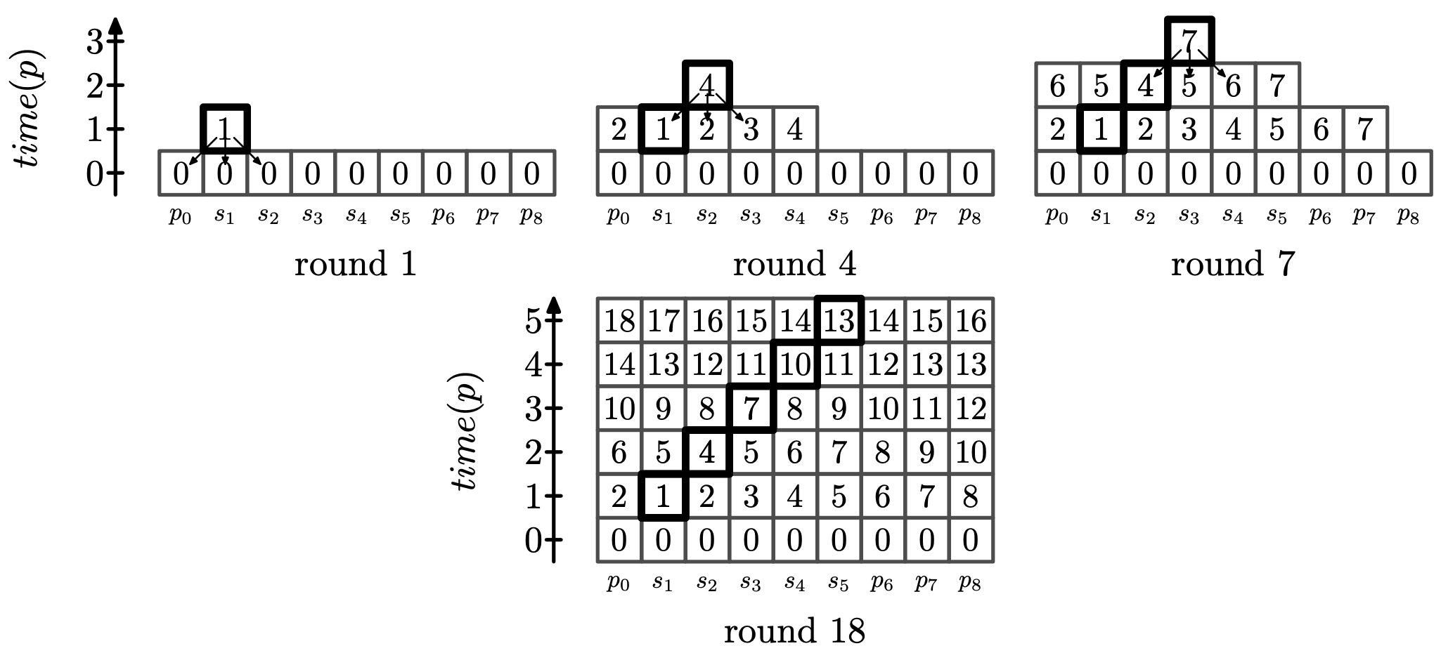
To give an intuition of our proof, as it is the more complex, we first consider the second stage. Figure 1 is an illustration of the following explanation. Suppose that all times are 0 in ${\gamma }^0$, and only $s_1$ is such that ${\text{st}}_{s_1}^0\ne {\text{st}}_{s_1}^1$. In the first round of the synchronous execution, $s_1$ applies $R_U$, and then, after each new round, nodes at distance 1 from $s_1$, then 2, and so on will increase their time to 1. Now suppose that only $s_2\in N[s_1]$ is such that ${\text{st}}_{s_2}^1\ne {\text{st}}_{s_2}^2$. As soon as all nodes in $N[s_2]$ have a time of 1, $s_2$ applies $R_U$. This happens at Round 3 if $s_2=s_1$ and at Round 4 otherwise. After this, after each new round, nodes at distance 1 from $s_2$, then 2, and so on will increase their time to 2. If we consider some $s_3\in N[s_2]$, and so on, then $s_i$ increases its time to $i$ at Round at most $3i-2$, and all nodes do so at Round at most $3i+D-2$. If nodes increase their time earlier, this only speed up the process.

Now, by definition of $H$, there is a node $s_H$ whose state changes between ${\lambda }_{H-1}$ and ${\lambda }_H$. If the states of all nodes in $N[p]$ were the same in ${\lambda }_{H-2}$ and ${\lambda }_{H-1}$, then $s_H$ would not have changed its state between ${\lambda }_{H-1}$ and ${\lambda }_H$. There thus exists $s_{H-1}\in N[s_H]$ that changes its state between ${\lambda }_{H-2}$ and ${\lambda }_{H-1}$. By repeating this process, we can prove that, unless $H=0$, $\mathrm{\Lambda }$ has a starting sequence that is a sequence $s_1\mathrm{\cdots }{s}_H$ verifying ${\text{st}}_{s_i}^{i-1}\ne {\text{st}}_{s_i}^i$ for $1\le i\le H$, and $s_{i-1}\in N[s_i]$ for . We can then prove that, if all nodes have a positive time at Round $X$, then the algorithm becomes silent after at most $X+3H+D-2$ rounds.

Using similar ideas, we can prove that all times are non-negative after at most $X=2D$ rounds. Taking into account the $3D+2$ rounds of the stabilization phase, we obtain an overall $5D+3T$ round complexity to reach the silence from any configuration.

References

- [1] S. Aggarwal and S. Kutten. Time optimal self-stabilizing spanning tree algorithms. In 13th Foundations of Software Technology and Theoretical Computer Science, (TSTTCS’93), volume 761, pages 400–410, 1993. doi:10.1007/3-540-57529-4_72.
- [2] K. Altisen, A. Cournier, S. Devismes, A. Durand, and F. Petit. Self-stabilizing leader election in polynomial steps. Information and Computation, 254(3):330–366, 2017. doi:10.1016/j.ic.2016.09.002.
- [3] K. Altisen, S. Devismes, S. Dubois, and F. Petit. Introduction to Distributed Self-Stabilizing Algorithms. Synthesis Lectures on Distributed Computing Theory. Morgan & Claypool, 2019. doi:10.2200/S00908ED1V01Y201903DCT015.
- [4] B. Awerbuch, S. Kutten, Y. Mansour, B. Patt-Shamir, and G. Varghese. Time optimal self-stabilizing synchronization. In 25th Annual Symposium on Theory of Computing, (STOC’93), pages 652–661, 1993. doi:10.1145/167088.167256.
- [5] B. Awerbuch, B. Patt-Shamir, and G. Varghese. Self-stabilization by local checking and correction. In 32nd Annual Symposium of Foundations of Computer, Science (FOCS’91), pages 268–277, 1991. doi:10.1109/SFCS.1991.185378.
- [6] B. Awerbuch and G. Varghese. Distributed program checking: a paradigm for building self-stabilizing distributed protocols. In 32nd Annual Symposium on Foundations of Computer Science, (FOCS’91), pages 258–267, 1991. doi:10.1109/SFCS.1991.185377.
- [7] Baruch Awerbuch. Complexity of network synchronization. J. ACM, 32(4):804–823, 1985. doi:10.1145/4221.4227.
- [8] J. Beauquier, M. Gradinariu, and C. Johnen. Cross-over composition - enforcement of fairness under unfair adversary. In 5th International Workshop on Self-Stabilizing Systems, (WSS’01), pages 19–34, 2001. doi:10.1007/3-540-45438-1_2.
- [9] L. Blin, C. Johnen, G. Le Bouder, and F. Petit. Silent anonymous snap-stabilizing termination detection. In 41st International Symposium on Reliable Distributed Systems, (SRDS’22), pages 156–165, 2022. doi:10.1109/SRDS55811.2022.00023.
- [10] C. Boulinier and F. Petit. Self-stabilizing wavelets and rho-hops coordination. In 22nd IEEE International Symposium on Parallel and Distributed Processing, (IPDPS’08), pages 1–8, 2008. doi:10.1109/IPDPS.2008.4536130.
- [11] C. Boulinier, F. Petit, and V. Villain. When graph theory helps self-stabilization. In 23rd Annual Symposium on Principles of Distributed Computing, (PODC’04), pages 150–159, 2004. doi:10.1145/1011767.1011790.
- [12] J. Burman and S. Kutten. Time optimal asynchronous self-stabilizing spanning tree. In 21st International Symposium on Distributed Computing, (DISC’07), volume 4731, pages 92–107, 2007. doi:10.1007/978-3-540-75142-7_10.
- [13] A. Cournier, A. K. Datta, F. Petit, and V. Villain. Snap-stabilizing PIF algorithm in arbitrary networks. In 22nd International Conference on Distributed Computing Systems (ICDCS’02), pages 199–206, 2002. doi:10.1109/ICDCS.2002.1022257.
- [14] A. Cournier, S. Rovedakis, and V. Villain. The first fully polynomial stabilizing algorithm for BFS tree construction. Information and Computation, 265:26–56, 2019. doi:10.1016/j.ic.2019.01.005.
- [15] J.-M. Couvreur, N. Francez, and M. G. Gouda. Asynchronous unison (extended abstract). In 12th International Conference on Distributed Computing Systems, (ICDCS’92), pages 486–493, 1992. doi:10.1109/ICDCS.1992.235005.
- [16] A. K. Datta, S. Devismes, K. Heurtefeux, L. L. Larmore, and Y. Rivierre. Competitive self-stabilizing -clustering. Theoretical Computer Science, 626:110–133, 2016. doi:10.1016/j.tcs.2016.02.010.
- [17] A. K. Datta, S. Devismes, and L. L. Larmore. A silent self-stabilizing algorithm for the generalized minimal k-dominating set problem. Theoretical Computer Science, 753:35–63, 2019. doi:10.1016/j.tcs.2018.06.040.
- [18] A. K. Datta and L. L. Larmore. Leader election and centers and medians in tree networks. In 15th International Symposium on Stabilization, Safety, and Security of Distributed Systems, (SSS’13), pages 113–132, 2013. doi:10.1007/978-3-319-03089-0_9.
- [19] S. Devismes, D. Ilcinkas, and C. Johnen. Optimized silent self-stabilizing scheme for tree-based constructions. Algorithmica, 84(1):85–123, 2022. doi:10.1007/s00453-021-00878-9.
- [20] S. Devismes, D. Ilcinkas, C. Johnen, and F. Mazoit. Making local algorithms efficiently self-stabilizing in arbitrary asynchronous environments. CoRR, abs/2307.06635, 2023. doi:10.48550/arXiv.2307.06635.
- [21] S. Devismes, D Ilcinkas, C. Johnen, and F. Mazoit. Asynchronous self-stabilization made fast, simple, and energy-efficient. In 43rd Symposium on Principles of Distributed Computing, (PODC’24), pages 538–548, 2024. doi:10.1145/3662158.3662803.
- [22] S. Devismes and C. Johnen. Silent self-stabilizing BFS tree algorithms revisited. Journal on Parallel Distributed Computing, 97:11–23, 2016. doi:10.1016/j.jpdc.2016.06.003.
- [23] S. Devismes and C. Johnen. Self-stabilizing distributed cooperative reset. In 39th International Conference on Distributed Computing Systems, (ICDCS’19), pages 379–389, 2019. doi:10.1109/ICDCS.2019.00045.
- [24] S. Devismes and F. Petit. On efficiency of unison. In 4th Workshop on Theoretical Aspects of Dynamic Distributed Systems, (TADDS’12), pages 20–25, 2012. doi:10.1145/2414815.2414820.
- [25] E. W. Dijkstra. Self-stabilization in spite of distributed control. Communications of the ACM, 17(11):643–644, 1974. doi:10.1145/361179.361202.
- [26] S. Dolev. Self-Stabilization. MIT Press, 2000.
- [27] S. Dolev, A. Israeli, and S. Moran. Self-stabilization of dynamic systems assuming only read/write atomicity. Distributed Computing, 7(1):3–16, 1993. doi:10.1007/BF02278851.
- [28] Y. Emek and E. Keren. A thin self-stabilizing asynchronous unison algorithm with applications to fault tolerant biological networks. In 40nd Symposium on Principles of Distributed Computing, (PODC’21), pages 93–102, 2021. doi:10.1145/3465084.3467922.
- [29] Y. Emek and R. Wattenhofer. Stone age distributed computing. In 32nd Symposium on Principles of Distributed Computing, (PODC’13), pages 137–146, 2013. doi:10.1145/2484239.2484244.
- [30] M. J. Fischer, N. A. Lynch, and M. S. Paterson. Impossibility of distributed consensus with one faulty process. Journal of the ACM, 32(2):374–382, 1985. doi:10.1145/3149.214121.
- [31] C. Glacet, N. Hanusse, D. Ilcinkas, and C. Johnen. Disconnected components detection and rooted shortest-path tree maintenance in networks. Journal of Parallel and Distributed Computing, 132:299–309, 2019. doi:10.1016/j.jpdc.2019.05.006.
- [32] Maria Gradinariu and Sébastien Tixeuil. Conflict managers for self-stabilization without fairness assumption. In 27th IEEE International Conference on Distributed Computing Systems (ICDCS 2007), June 25-29, 2007, Toronto, Ontario, Canada, page 46. IEEE Computer Society, 2007. doi:10.1109/ICDCS.2007.95.
- [33] A. Kravchik and S. Kutten. Time optimal synchronous self stabilizing spanning tree. In 27th International Symposium on Distributed Computing, (DISC’13), pages 91–105, 2013. doi:10.1007/978-3-642-41527-2_7.
- [34] S. Tixeuil. Vers l’auto-stabilisation des systèmes à grande échelle. Habilitation à diriger des recherches, Université Paris Sud - Paris XI, 2006. URL: https://tel.archives-ouvertes.fr/tel-00124848/file/hdr_final.pdf.
- [35] V. Turau. Efficient transformation of distance-2 self-stabilizing algorithms. Journal of Parallel and Distributed Computing, 72(4):603–612, 2012. doi:10.1016/j.jpdc.2011.12.008.