Two-Dimensional Longest Common Extension Queries in Compact Space

Abstract
For a length text over an alphabet of size , we can encode the suffix tree data structure in bits of space. It supports suffix array (), inverse suffix array (), and longest common extension () queries in time, which enables efficient pattern matching; here is an arbitrarily small constant. Further improvements are possible for queries, where time queries can be achieved using an index of space bits. However, compactly indexing a two-dimensional text (i.e., an matrix) has been a major open problem. We show progress in this direction by first presenting an -bit structure supporting queries in near time. We then present an -bit structure supporting queries in near time. Within a similar space, achieving queries in poly-logarithmic (even strongly sub-linear) time is a significant challenge. However, our -bit structure can support queries in time, where is an arbitrarily large constant, which enables pattern matching in time faster than what is possible without preprocessing.
We then design a repetition-aware data structure. The compressibility measure for two-dimensional texts was recently introduced by Carfagna and Manzini [SPIRE 2023]. The measure ranges from to , with smaller indicating a highly compressible two-dimensional text. The current data structure utilizing allows only element access. We obtain the first structure based on for queries. It takes space and answers queries in time.
Keywords and phrases:
String matching, text indexing, two-dimensional textCopyright and License:
2012 ACM Subject Classification:
Theory of computation Pattern matchingFunding:
Supported by the US National Science Foundation (NSF) under Grant Numbers 2315822 (S Thankachan) and 2137057 (R Shah).Editors:
Olaf Beyersdorff, Michał Pilipczuk, Elaine Pimentel, and Nguyễn Kim ThắngSeries and Publisher:
1 Introduction
A two-dimensional text can be viewed as an matrix, where each entry is a character from an alphabet set of size . Data structures for two-dimensional texts have been studied for decades. In particular, there has been extensive work on generalizing suffix trees [16, 17, 23] and suffix arrays [16, 22] to 2D text. These data structures, although capable of answering most queries in optimal (or near optimal) time, require words, or bits, of space.
On the other hand, in the case of 1D texts of length , there exist data structures with the same functionality as suffix trees/arrays but requiring only bits of space [18, 32], or even smaller in the case where the text is compressible [11, 21]. This is true even for some variants of suffix trees, such as parameterized [14, 13] and order-isomorphic [12] suffix trees [33]. The query times of these space-efficient versions are often polylogarithmic, with the exception of queries, for which Kempa and Kociumaka demonstrated that the query time can be made constant [19]. For 2D texts, the only results known in this direction include a data structure by Patel and Shah that uses bits and supports inverse suffix array () queries in time [28]. In this work, we make further progress in this direction. In particular, we focus on space-efficient data structures for longest common extension () queries in the 2D setting. The problem is formally defined as follows:
Problem 1 (2D LCE).
Preprocess a 2D text over an alphabet of size into a data structure that can answer 2D LCE queries efficiently. A 2D LCE query consists of points , and asks to return the largest such that and are matching square submatrices of .
A 2D suffix tree of size bits can answer queries in constant time. Our first result is an data structure that occupies bits of space.
Theorem 1.
By maintaining an -bit data structure, we can answer 2D LCE queries in time.
Turning now to highly compressible 2D texts, we consider repetition-aware compression measures. The measure is an important and well-studied compressibility measure for 1D text [26]. Only recently has it been extended to 2D text by Carfagna and Manzini with a -measure [5]. They demonstrate that the data structure of Brisaboa et al. [3] occupies space. However, this data structure only supports access to the elements of . We provide the first repetition-aware data structure supporting the more advanced queries. Note that the measure ranges from to , with a smaller value implying higher compressibility.
Theorem 2.
By maintaining an word data structure, we can answer 2D LCE queries in time, where is always and goes to as approaches . In particular,
When , our data structure takes words of space and answers queries in time. When , the space becomes and queries are answered in logarithmic time. Our approach builds off many of the same techniques as our compact index but also introduces a matrix representation of the leaves of a truncated suffix tree. We call this a macro-matrix. We prove that if the original 2D text is compressible, then this macro-matrix remains compressible for appropriately chosen parameters. This is then combined with the data structure of Brisaboa et al. [3] to achieve Theorem 2.
As the first steps towards obtaining the other functionalities of the suffix tree, we apply our 2D LCE query structure from Theorem 1 to get the following results. Definitions of suffix array () and inverse suffix array () are deferred to Section 1.1.
The following theorem significantly improves on the results by Patel and Shah [28].
Theorem 3 (2D ISA queries).
By maintaining an -bit data structure, we can answer inverse suffix array queries in time.
We also provide the first known results regarding a nearly compact index for 2D suffix array queries.
Theorem 4 (2D SA queries).
By maintaining an -bit data structure, we can answer suffix array (SA) queries in time, where is an arbitrarily large constant fixed at the time of construction.
A fundamental problem is to find all submatrices of that match with a given square pattern . After building the 2D suffix tree, given as a query, the number of occurrences of (denoted by ) can be obtained in time, and all occurrences can be reported in time. Our result, which uses a smaller index, is the following.
Theorem 5 (PM queries).
By maintaining an -bit data structure, we can count the occurrences of an query pattern in time and report all occurrences in time , where is an arbitrarily large constant fixed at the time of construction.
Although the time complexities in Theorems 4 and 5 are far from satisfactory, these are the first results demonstrating subquadratic query times in compact space are possible for 2D and PM queries.
1.1 Preliminaries
Notation and Strings.
We denote the interval , , , with and the interval , , , , with . For a string of length we use to refer to character, . We use to denote the concatenation of two strings and . For notation, , , and . Arrays and strings are zero-indexed throughout this work.
For a single string and , is defined as the length of the longest common prefix of and . In the case of two strings, and , we overload the notation so that for , , is the length of the longest common prefix of and . For a given string , the suffix tree [34] is a compact trie of all suffixes of with leaves ordered according to the lexicographic rank of the corresponding suffixes. The classical suffix tree takes words of space and can be constructed in time for polynomially sized integer alphabets [9]. The suffix array of a string is the unique array such that is the smallest suffix lexicographically. The inverse suffix array is the unique array such that , or equivalently, gives the lexicographic rank of . The suffix tree can answer queries in time. We call a compact trie with lexicographically ordered leaves for a subset of suffixes a sparse suffix tree. Observe that the number of nodes in a sparse suffix tree remains proportional to the number of suffixes it is built from.
We will utilize the following result by Kempa and Kociumaka, which provides an data structure smaller than a classical suffix tree.
Lemma 6 ([19]).
1D LCE queries on a text over an alphabet set can be answered in time by maintaining a data structure of size bits.
The next result by Bille et al. allows for a trade-off between space and query time. We will utilize it in Section 2.2.
Lemma 7 ([1]).
Suppose we have the text as read-only, such that we can determine the lexicographic order of any of its two characters in constant time. Then we can answer 1D LCE queries on in time by maintaining an words of space auxiliary structure, where is any parameter fixed at the time of construction.
d-Covers.
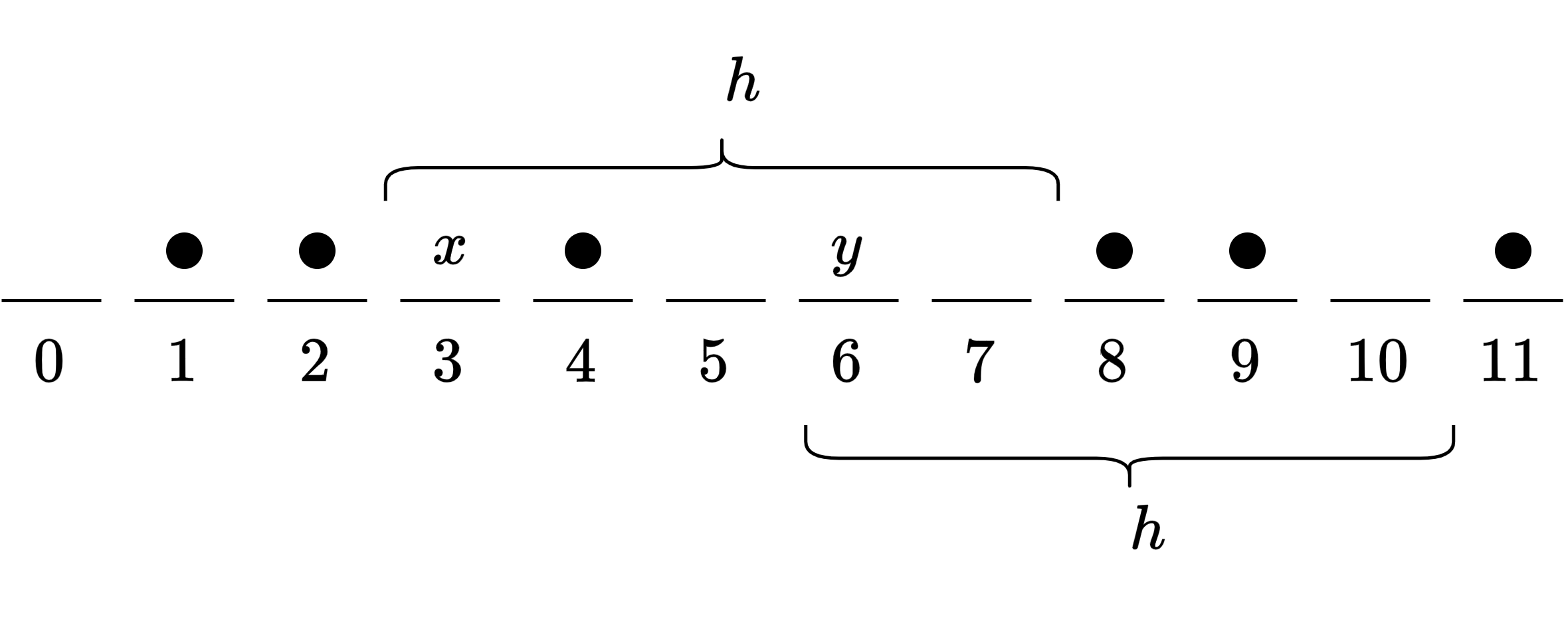
A -cover of an interval is a subset of positions, denoted by , such that for any and there exists where . It was shown by Burkhardt and Kärkkäinen that there exists a -cover of size that can be computed in time [4]. -Covers have been used previously for LCE queries in the 1D case by Gawrychowski et al. [15] and Bille et al. [2]. Since we need a small data structure that lets us find an value as described above in constant time, we briefly outline the construction given in [4].
A difference cover modulo is a subset where for all there exist such that . Colbourn and Ling showed there exists such that [8]. A -cover is constructed from a difference cover as follows: For , if , then is added to . We also build a look-up table of size such that for all both and are in . This is always possible, thanks to the definition of the difference cover. See Figure 1.

Lemma 8 ([4]).
For a -cover of an interval , there exists a data structure of size that given , outputs an such that in time.
Proof.
We maintain the space look-up table as described above. We assume without loss of generality, . Let . Observe that
Hence, and . Also,
Hence, and .
2D Suffix Trees and 2D Suffix Arrays.
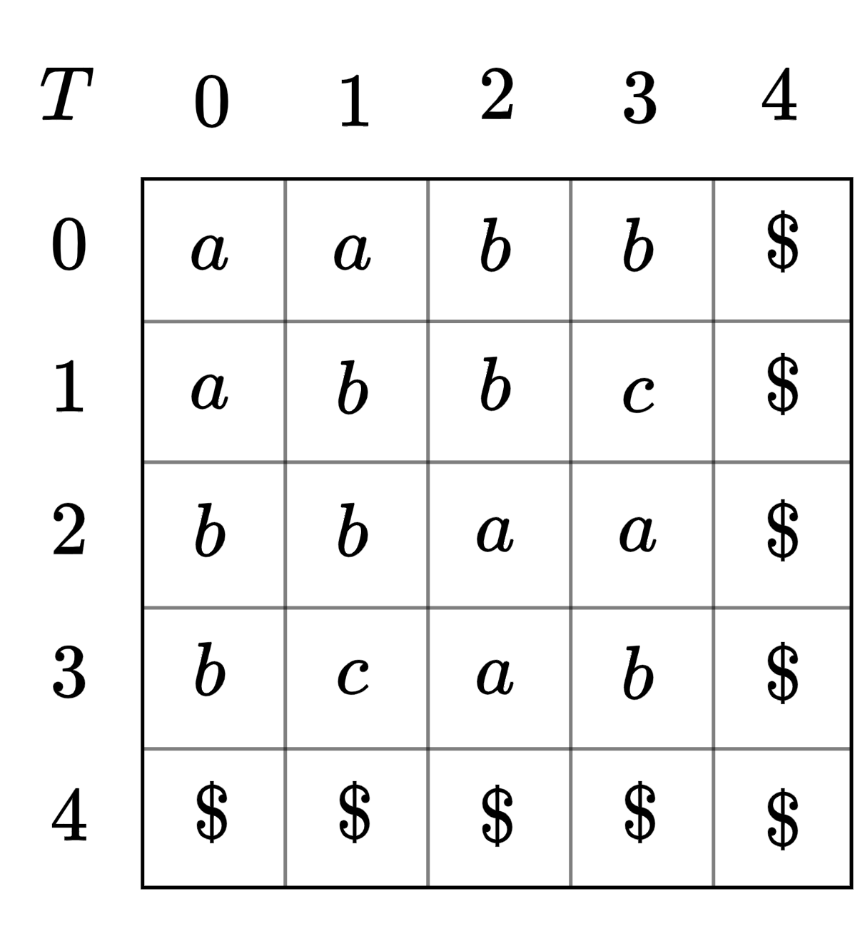
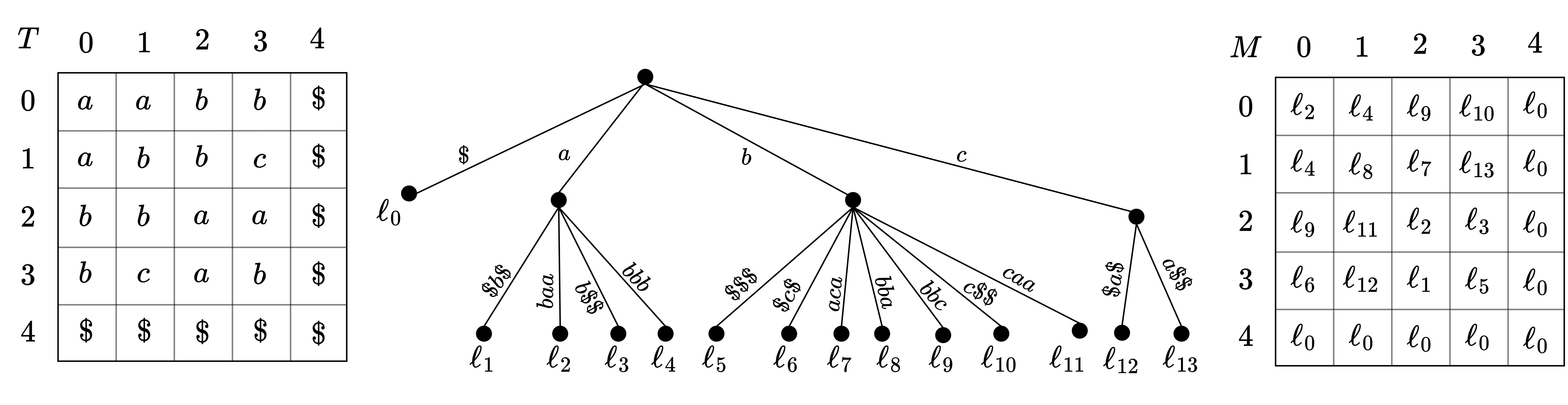
We utilize the generalization of suffix trees to 2D texts presented by Giancarlo [16]. This suffix tree is created from the Lstrings of the 2D text . LStrings are over an alphabet . For a position the suffix is where and and for . See Figure 2. The characters are maintained implicitly as references to , resulting in the 2D suffix tree over all suffixes , occuping words of space. Once constructed, the 2D suffix tree allows us to find the of two positions in time through a lowest common ancestor () query. The 2D suffix tree also enables pattern matching in optimal time.
The order between characters and of Lstrings is defined as the lexicographic order induced by the base alphabet . The lexicographic order of two Lstrings (and corresponding submatrices) is induced by the order of their characters. We additionally assume that the bottom row and rightmost column of consist of only a symbol, which is the smallest in the alphabet order and occurs nowhere else in .
| suffix starting at : | |||
| suffix starting at : | |||
| suffix starting at : |
The suffix array of a 2D text is an array containing 2D points such that if , then is the smallest suffix lexicographically. The inverse suffix array maps each to its position in , i.e. .
The Measure and 2D Block Trees.
The measure is a well-studied compressibility measure for 1D texts [7, 20, 24, 25, 30]. It is defined as where denotes the number of distinct length substrings of .
Carfagna and Manzini recently generalized the measure to 2D texts [5, 6]. Letting denote the number of distinct submatrices of , . Observe that can range between , e.g., in case where all elements of are the same character, and , i.e., the case where all elements of are distinct. Carfagna and Manzini showed that the 2D block tree data structure of Brisaboa, et al. [3] occupies words of space and provides access to any entry of in time. A further generalization of the measure to 2D allowing for non-square matrices was introduced by Romana et al. and related to other potential 2D compressibility measures [31]. In this work, we will only consider the measure based on square submatrices. We hereafter refer to as and omit the text when it is clear from context.
2 Compact Data Structures for 2D LCE Queries
We start with some definitions. Let denote the row and denote the column of our 2D text , where . Specifically, (resp., ) is a text of length over the alphabet , such that its character is (resp., ), where .
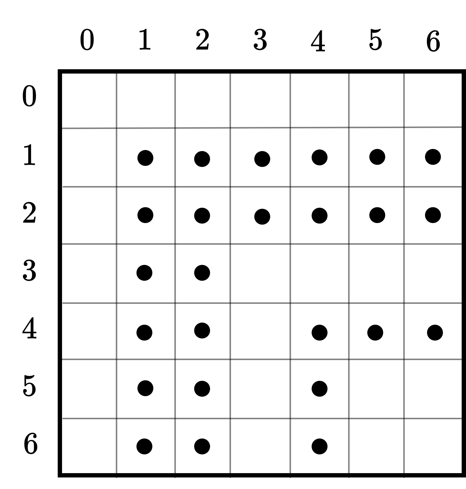
We define a set of sampled positions on the diagonals of , that is , , , , , using -cover with . This is obtained by taking a -cover for and using it to define sample positions starting from the top left of each diagonal. Formally, the sample positions are
See Figure 3.
We maintain a sparse suffix tree over the suffixes starting from these sampled positions. As this is a compact trie with leaves, the space required for this sparse suffix tree is words. By our above choice of , this is bits. Using this sparse suffix tree, we can obtain for any two sampled positions in time.
Additionally, we maintain the data structure from Lemma 6 for the concatenation of columns , , and rows , , , which adds another bits. This allows us to find the between and (or and ) in time. We can take a minimum between the value and to avoid common prefixes crossing row or column boundaries.
In what follows, we first present a simple preliminary solution. We then develop these ideas further with two refinements that lead us to Theorem 1. The components defined above (sparse suffix tree from diagonal samples and data structures for concatenated rows and columns) are used in all three solutions.
2.1 Achieving Query Time
To answer an query , , we use the look-up structure discussed in Lemma 8 to obtain an such that and are sampled diagonal positions. For convenience, in the case where no such in the look-up structure exists, because either or is near the boundary of , we consider as being one less than the minimum diagonal offset to a boundary of . We first obtain in time. Next, for , we compute the s between and , and between and . While iterating from to , if for some either the between and or between and becomes less than , we output . Otherwise, we output the minimum over and all of the values computed for the rows and columns specified above.
Only one constant time query for a diagonal sampled position is required, and the number of 1D LCE queries needed is at most . Since and each 1D LCE query takes time, the total time is .
2.2 Achieving Query Time
First, we define and . These are texts of length over an alphabet , such that and . The character of and are length strings over defined as follows:
We call these meta characters. We also call and slabs of length . Applying the structure from Lemma 6 over the concatenation of rows and the concatenation of columns, we can compare two meta characters in time.
Data Structure.
Querying.
Given an query , , we first find an such that and are sampled positions. We then decompose the interval and into slabs that have lengths that are powers of two. We perform an query for each corresponding slab for both rows and columns. A minimum is taken over all these values and . Denote this minimum with . There are two possible cases.
-
. See Figure 4(a). In this case, is reported as the result.
-
. See Figure 4(b). In this case, we still need to find the largest value such that the minimum of the slabs covering , , (with slabs covering ,, , respectively) and , , (with slabs covering , , , respectively) is at least . To accomplish this, we perform a modified binary search while keeping track of the minimum values for both the column and row slabs. The only difference compared to standard binary search is that rather than always dividing the current range under consideration in half, we consider the power of two closest to half the size of the current range. This is done to ensure that we always use slabs for which we have prepared data structures.
Analysis.
Letting be the number of queries on slabs for the binary search on a range of length , the resulting recurrence is
Hence, . We now fix . Since each query on a slab takes time, the overall query time is , where we used that . The total added space relative to the previous solution is words. Using our definitions of and , the space remains bits.
2.3 Achieving Query Time
Data Structure.
Let be a parameter to be defined later. In addition to the previously defined diagonal sample positions, we now define sample positions for the rows and columns using an -cover, denoted by . We maintain the structure in Lemma 7 (with parameter left open for optimizing later) over the text obtained by concatenating slabs for , whenever . We do the same for slabs for whenever and . Similarly, we maintain the structure from Lemma 7 for the concatenation of for for . We do the same for for whenever and . Note that these slabs do not need to be explicitly constructed and can be simulated directly using the input text.
Querying.
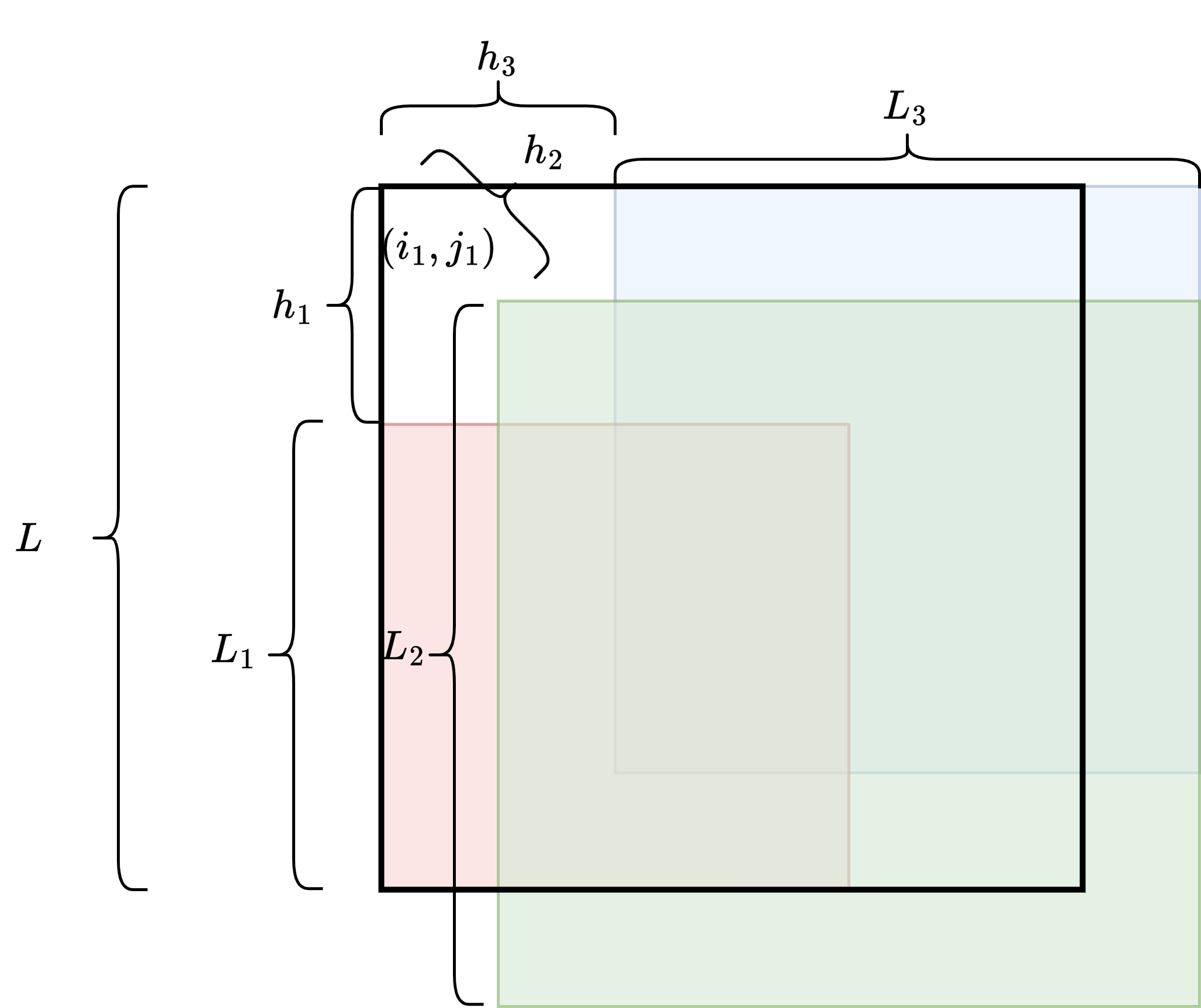
Given a query , , we first find such that and are diagonal sample positions. Let find such that and are in . We find the s of columns , , with , , , respectively. We next find such that and are in . We then find the s of columns , , with , , , respectively. We then take the largest power of two, say , such that , and obtain the of the slab with . We also obtain the of the slabs and . We perform a symmetric procedure on the rows. A minimum is taken among all of these values as well as . Let denote this minimum. We consider two cases like in Section 2.2.
-
. In this case, is reported as the result.
-
. As in Section 2.2, we want to output the largest value such that the minimum of the slabs covering , , (with relative to slabs covering ,, ) and , , (with relative to slabs covering , , ) is at least . The modification to the binary search algorithm from Section 2.2 is that we intermix at most single row/column evaluations to reach the next position in . After this position in is reached, the power of two that most evenly splits the remaining range can be used.
Analysis.
We claim that answering a query requires number of LCE queries for single rows/columns and number of LCE queries on slabs. To see this, let be the number of single row/column queries on a range of length , and be the number of slab queries. Then we have
Hence, and . Each single row/column query takes time and each query on a slab takes time. As a result, the total query time is . To optimize, we keep and now fix and obtain the query time of .
3 Repetition-Aware LCE Data Structure
Overview.
We use a parameter that we will optimize over later. We aim to use a truncated suffix tree in conjunction with a sparse suffix tree on sampled positions from a -cover to efficiently perform queries. If we truncate the 2D suffix tree at a string depth of , then the measure provides an upper bound of on the number of leaves at depth . As we argue, one can also upper bound the number of additional leaves in the truncated suffix tree in terms of and .
The first challenge in using the above ideas is that, for these queries from sampled positions to provide information on the overall result, the matching submatrices starting at sampled positions should overlap. This is accomplished by using a string depth of for the truncated suffix tree while still using a -cover. The second challenge is that given our query, we need to know which leaves to consider in the truncated suffix tree. Moreover, we should accomplish this in space when is small. To this end, we introduce the notion of a macro-matrix , which stores the leaf in the truncated suffix tree to examine for a specified position in . We then relate the measure of this macro-matrix to the measure of the matrix . This relationship enables us to use the 2D block tree data structure of Brisboa et al. [3] on , which occupies sublinear space for compressible matrices and supports efficient access to the elements of .
3.1 Data Structures
Truncated Suffix Tree.
We first construct a 2D suffix tree of truncated at a string depth of . Call this . We use , , to denote the leaves of .
Compressed Representation of Macro-Matrix.
We next define the macro-matrix. The elements of a macro-matrix are essentially meta symbols, where two meta-symbols are the same if and only if the corresponding square substrings are identical. Formally, the macro-matrix is the matrix obtained as follows: for ,
-
if there exists a matrix with upper left corner , i.e., , then we make where is a pointer to the leaf of corresponding to ;
-
if or , then let where is a pointer to the leaf in corresponding to the matrix with upper left corner .
See Figure 5. We then construct the 2D block tree of , denoted as .
Sparse Suffix Tree.
We define sample positions based on a -cover of . These consist of sample positions for the rows,
for the columns,
and for the diagonals,
Let . Observe that . We build a sparse suffix tree over the suffixes starting at sampled positions in , denoted as . We also maintain the lookup data structure from Lemma 8. As before, this allows us to find in time equally far sampled positions at most away from the queried positions in each row, column, and diagonal.
3.2 Querying
Given query , , we first use to get the corresponding values in . Say these correspond to the leaves and in respectively. If , then the string depth of the of and gives us the of , .
If then we use the lookup data structure from Lemma 8 to find:
-
such that and are sampled positions. We then use an time query on to get the of and . Denote this value as .
-
such that and are sampled positions. We use an time query on to get the of and . Denote this value as .
-
such that and are sampled positions. We use an time query on to get the of and . Denote this value as .
We report as the solution.
3.3 Correctness
The first lemma is immediate.
Lemma 9.
When , is the string depth of .
Lemma 10.
When , .
Proof.
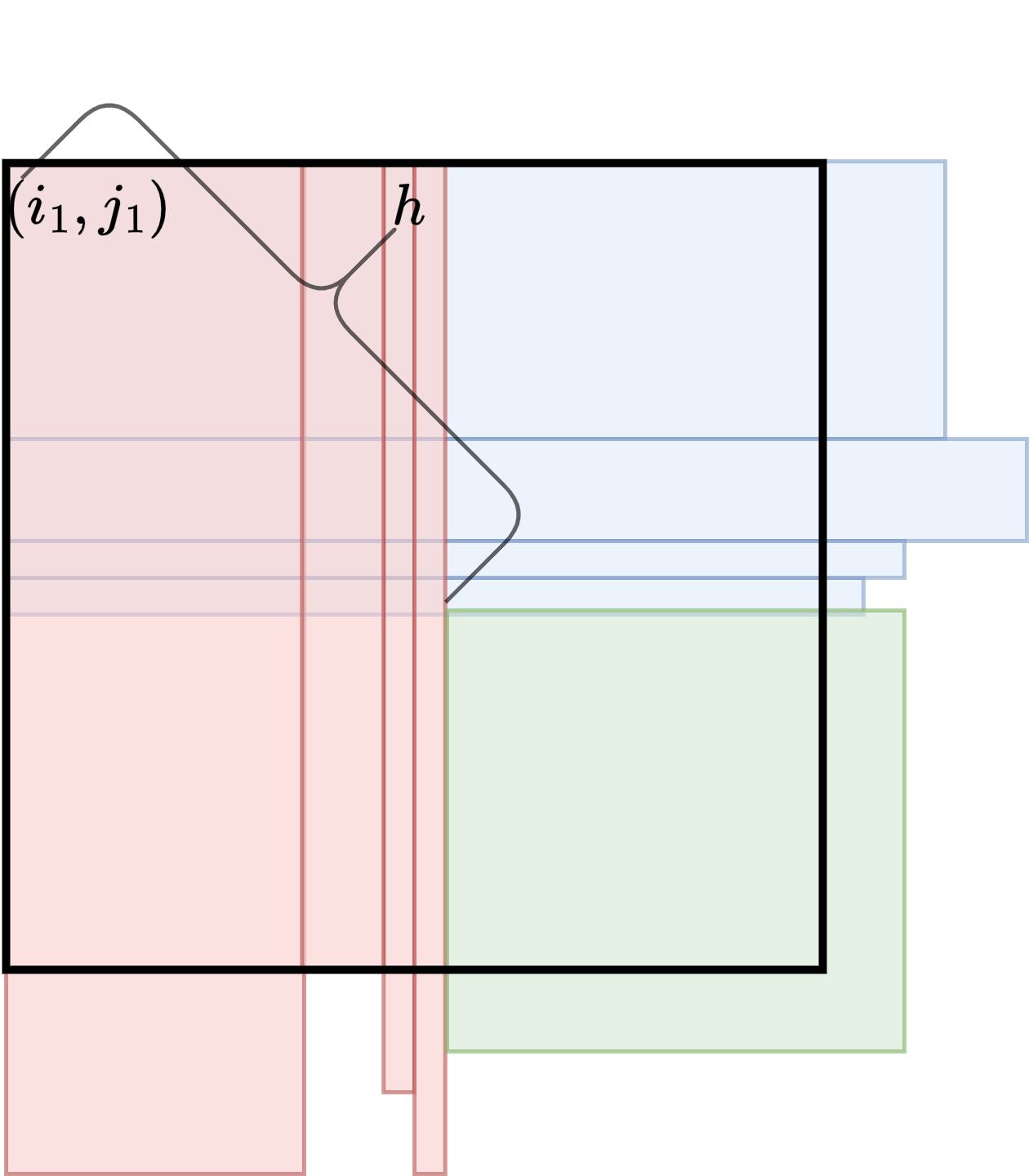
Define . First, we show that . Starting from there exists a matching submatrix (with respect to position ) of size at least , thus we have that . Hence, . A similar argument holds for and .
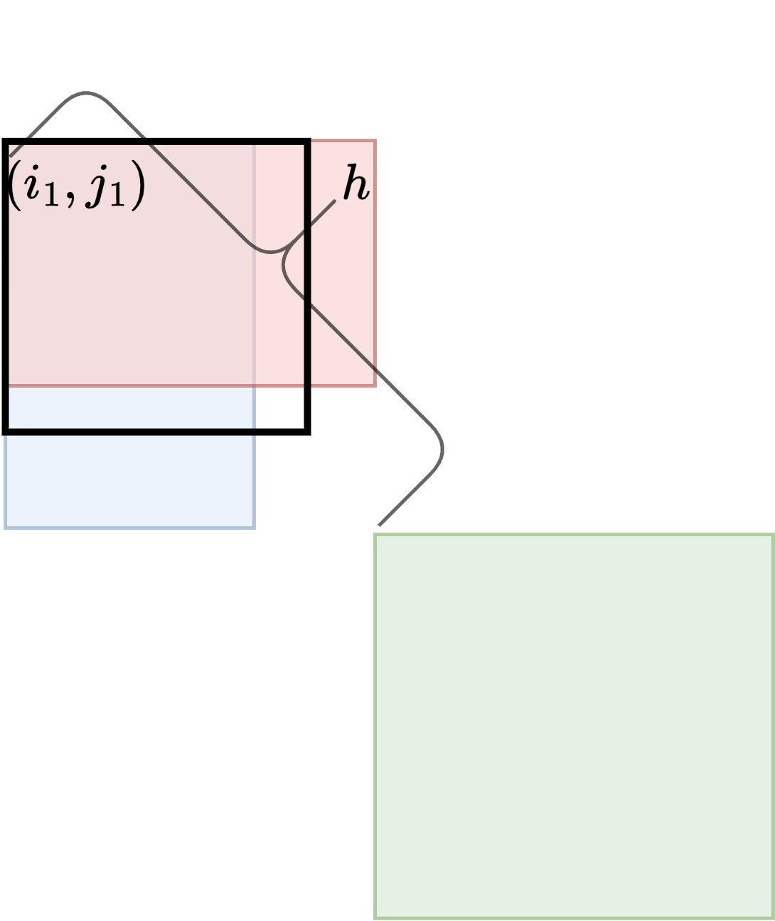
Next, we show .
-
We denote the submatrix as .
-
We denote the submatrix as .
-
We denote the submatrix as
See Figure 6.
Observe that and since , we have . Submatrix has lower left corner in column and in row making it overlap with . Also, has upper right corner in column and row . Hence, overlaps with as well.
Now, suppose for the sake of contradiction that . For any positions in row and column where we have
and
Similarly, for any position in column and row where we have
and
Based on the above inequalities and the fact that submatrices , , and overlap, this implies that the matching submatrices with upper left corners and can be extended further by at least one row and column. This contradicts the definition of .
3.4 Analysis and Optimization
3.4.1 Space Analysis
Space for -Cover lookup structure and Sparse Suffix Tree.
According to Lemma 8, the lookup structure requires space. Since , we have that the sparse suffix tree uses space.
Space for .
The space for the truncated suffix tree is bounded by the number of distinct submatrices of , denoted , plus the number of distinct matrices of size less than that can not be further extended down and to the right (due to a boundary of ). There are at most of the latter since, for every length from to , at most submatrices cannot be further extended. By the definition of , , making the space for bound by .
Space for Macro-Matrix.
The space for depends on . We prove the following lemma relating and .
Lemma 11.
and .
Proof.
First, the lower bound. Observe that for an arbitrary , two matching submatrices in cause two matching submatrices in (with the same upper left corners as the corresponding submatrices in ). In this way, every distinct submatrix in maps to one distinct submatrix in , and we have . Then for , we have
| (1) |
implying for .
Next, consider . Note that the number of distinct submatrices in is almost upper bounded by the number of distinct submatrices in , except that some of the distinct matrices with sizes between and may be prevented from being extended due to the right and bottom boundaries of . The number of such submatrices is bounded by . Hence, for ,
Applying Inequality (1), we can then write
Taking the maximum over both cases, yields that .
For the upper bound, we claim that, for an arbitrary ,
where we take if . The above inequality follows from the fact that every distinct submatrix in maps to one distinct submatrix in . What remains to be counted for are distinct submatrices in that are not resulting from some submatrix in . That is, submatrices on the bottom and/or right boundary. Again, the number of such submatrices is bounded by .
To complete the proof, we have the bound
Let be the alphabet size of the macro-matrix . The space for the block tree is
Applying that and Lemma 11, this space is bound by
Total Space.
Summing the total data structure sizes, the combined space is
3.4.2 Optimizing
We consider two cases based on , which we now denote as just . If , we set and let . The space is (up to constant factors)
Observe that as approaches , approaches .
If , we make . The resulting space complexity is
For this case, the argument of the logarithm is . One can also readily check that as defined above is bound by the expression for appearing in Theorem 2.
3.4.3 Query Time
The query time is dominated by the access to , which takes time, where is defined as above. The remaining queries take time. This completes the proof of Theorem 2.
4 Applications
4.1 ISA Queries
We maintain a sampled suffix array. Specifically, we sample the suffix array values for every leaf of the suffix tree. The space required for this is bits. Additionally, for each text position, we maintain how far away its predecessor sampled leaf is relative to its leaf in the suffix tree. This requires bits per entry. The resulting total space is bits.
To find the value of a text position , we perform a binary search on the sampled leaves to find the lexicographic predecessor of within the sampled set. Once the predecessor is found, we add the offset associated with . This gives us the suffix array position associated with , i.e., its value. The binary search requires number of queries. Each query takes time, resulting in an overall time complexity of .
4.2 SA queries
Let be a parameter. We divide the leaves of the suffix tree into contiguous blocks of size (except for perhaps the last block, which can be smaller). There are blocks. We associate each position in with the block in which its leaf lies in the suffix tree. This information is stored as follows: consider a binary array associated with each block . Each binary array is of length and represents a linearization of . For a block , we consider a in a position if the corresponding suffix tree leaf is in block and otherwise. Note that there are at most ’s in . We build a data structure representing using bits of space, or equivalently, bits of space, such that select queries can be answered in constant time [29]. The total space for select data structures over all bit vectors, is bits. We also maintain the data structure described previously.
Given an query for index , we first identify which block is in. Say this is block . We use select queries to iterate through the text positions contained in block . For each text position iterated over, we perform an query and check whether its value equals .
The space required for the data structure is bits. The space for the select data structures is bits. The query time is . We obtain Theorem 4 by making , where is an arbitrarily large constant that can absorb the additional logarithmic factors in the query time.
4.3 Pattern Matching
Counting.
In addition to the previous structures, we maintain the LCE data structure from Lemma 6 over the rows and columns. First, a binary search is done to find the leaf for the lexicographically smallest suffix with as a prefix (if one exists). We start by using an query to obtain . Using that we have read access to the original text, we match characters in in Lstring order to the submatrix starting at until we reach our first mismatch. At this point, we know our lexicographical order relative to our current leaf. When we transition to a new leaf in the binary search, we perform an query followed by queries with the position from the preceding leaf. This avoids repeatedly iterating over characters in . Assuming the query is at least the length already matched, we continue matching from the last matched position. A similar binary search finds the lexicographically largest suffix with as a prefix. We return the suffix range length.
The total number of and queries performed is . The time is dominated by the queries, which require time.
Reporting.
We start with the suffix range obtained previously, say . We use the same blocking scheme for the suffix leaves described for queries, also using constant time select data structures. We first identify the block that lies in, say . We use the select data structure to iterate through all of the text positions corresponding to suffixes in block . For each position, we perform an query and check whether its position in the suffix array is at least . If it is, we output it. We perform a similar procedure for the block containing , now checking if the position in the suffix array is at most . For the remaining blocks, those completely contained in , we use their select data structures to output all occurrences with suffixes in that block.
The space complexity is the same as the data structure. For the query time, each block has size , and with , the time spent on the blocks containing and is absorbed by already appearing due to queries.
5 Open Problems
We leave open many directions for potential improvement, for example:
-
Can we design a data structure with faster query time that uses bits of space (or better)? This seems significantly harder than queries. Suffix array sampling, like in the FM-index [10], is not immediately adaptable.
-
Can we design a data structure in repetition-aware compressed space that supports , , or pattern-matching queries? Also, can the space for a data structure for queries be improved? Grammar-based compression has proven useful for repetition-aware compressed data structures supporting queries in the 1D case, particularly run-length straight-line programs (RL-SLP). For 1D text, it is possible to construct RL-SLPs with size close to the measure [25], which can be used for [27] and pattern matching queries [24]. Although Romana et al. [31] introduce a version of RL-SLP for 2D text, it is open how such a RL-SLP could be utilized for queries and other types of queries, e.g., and pattern matching queries.
References
- [1] Philip Bille, Inge Li Gørtz, Mathias Bæk Tejs Knudsen, Moshe Lewenstein, and Hjalte Wedel Vildhøj. Longest common extensions in sublinear space. In Ferdinando Cicalese, Ely Porat, and Ugo Vaccaro, editors, Combinatorial Pattern Matching - 26th Annual Symposium, CPM 2015, Ischia Island, Italy, June 29 - July 1, 2015, Proceedings, volume 9133 of Lecture Notes in Computer Science, pages 65–76. Springer, 2015. doi:10.1007/978-3-319-19929-0_6.
- [2] Philip Bille, Inge Li Gørtz, Benjamin Sach, and Hjalte Wedel Vildhøj. Time-space trade-offs for longest common extensions. J. Discrete Algorithms, 25:42–50, 2014. doi:10.1016/J.JDA.2013.06.003.
- [3] Nieves R. Brisaboa, Travis Gagie, Adrián Gómez-Brandón, and Gonzalo Navarro. Two-dimensional block trees. Comput. J., 67(1):391–406, 2024. doi:10.1093/COMJNL/BXAC182.
- [4] Stefan Burkhardt and Juha Kärkkäinen. Fast lightweight suffix array construction and checking. In Ricardo A. Baeza-Yates, Edgar Chávez, and Maxime Crochemore, editors, Combinatorial Pattern Matching, 14th Annual Symposium, CPM 2003, Morelia, Michocán, Mexico, June 25-27, 2003, Proceedings, volume 2676 of Lecture Notes in Computer Science, pages 55–69. Springer, 2003. doi:10.1007/3-540-44888-8_5.
- [5] Lorenzo Carfagna and Giovanni Manzini. Compressibility measures for two-dimensional data. In Franco Maria Nardini, Nadia Pisanti, and Rossano Venturini, editors, String Processing and Information Retrieval - 30th International Symposium, SPIRE 2023, Pisa, Italy, September 26-28, 2023, Proceedings, volume 14240 of Lecture Notes in Computer Science, pages 102–113. Springer, 2023. doi:10.1007/978-3-031-43980-3_9.
- [6] Lorenzo Carfagna and Giovanni Manzini. The landscape of compressibility measures for two-dimensional data. IEEE Access, 12:87268–87283, 2024. doi:10.1109/ACCESS.2024.3417621.
- [7] Anders Roy Christiansen, Mikko Berggren Ettienne, Tomasz Kociumaka, Gonzalo Navarro, and Nicola Prezza. Optimal-time dictionary-compressed indexes. ACM Trans. Algorithms, 17(1):8:1–8:39, 2021. doi:10.1145/3426473.
- [8] Charles J. Colbourn and Alan C. H. Ling. Quorums from difference covers. Inf. Process. Lett., 75(1-2):9–12, 2000. doi:10.1016/S0020-0190(00)00080-6.
- [9] Martin Farach. Optimal suffix tree construction with large alphabets. In 38th Annual Symposium on Foundations of Computer Science, FOCS ’97, Miami Beach, Florida, USA, October 19-22, 1997, pages 137–143. IEEE Computer Society, 1997. doi:10.1109/SFCS.1997.646102.
- [10] Paolo Ferragina and Giovanni Manzini. Opportunistic data structures with applications. In 41st Annual Symposium on Foundations of Computer Science, FOCS 2000, 12-14 November 2000, Redondo Beach, California, USA, pages 390–398. IEEE Computer Society, 2000. doi:10.1109/SFCS.2000.892127.
- [11] Travis Gagie, Gonzalo Navarro, and Nicola Prezza. Fully functional suffix trees and optimal text searching in BWT-runs bounded space. J. ACM, 67(1):2:1–2:54, 2020. doi:10.1145/3375890.
- [12] Arnab Ganguly, Dhrumil Patel, Rahul Shah, and Sharma V. Thankachan. LF successor: Compact space indexing for order-isomorphic pattern matching. In Nikhil Bansal, Emanuela Merelli, and James Worrell, editors, 48th International Colloquium on Automata, Languages, and Programming, ICALP 2021, July 12-16, 2021, Glasgow, Scotland (Virtual Conference), volume 198 of LIPIcs, pages 71:1–71:19. Schloss Dagstuhl – Leibniz-Zentrum für Informatik, 2021. doi:10.4230/LIPICS.ICALP.2021.71.
- [13] Arnab Ganguly, Rahul Shah, and Sharma V. Thankachan. pbwt: Achieving succinct data structures for parameterized pattern matching and related problems. In Philip N. Klein, editor, Proceedings of the Twenty-Eighth Annual ACM-SIAM Symposium on Discrete Algorithms, SODA 2017, Barcelona, Spain, Hotel Porta Fira, January 16-19, pages 397–407. SIAM, 2017. doi:10.1137/1.9781611974782.25.
- [14] Arnab Ganguly, Rahul Shah, and Sharma V. Thankachan. Fully functional parameterized suffix trees in compact space. In Mikolaj Bojanczyk, Emanuela Merelli, and David P. Woodruff, editors, 49th International Colloquium on Automata, Languages, and Programming, ICALP 2022, July 4-8, 2022, Paris, France, volume 229 of LIPIcs, pages 65:1–65:18. Schloss Dagstuhl – Leibniz-Zentrum für Informatik, 2022. doi:10.4230/LIPICS.ICALP.2022.65.
- [15] Pawel Gawrychowski, Tomasz Kociumaka, Wojciech Rytter, and Tomasz Walen. Faster longest common extension queries in strings over general alphabets. In Roberto Grossi and Moshe Lewenstein, editors, 27th Annual Symposium on Combinatorial Pattern Matching, CPM 2016, June 27-29, 2016, Tel Aviv, Israel, volume 54 of LIPIcs, pages 5:1–5:13. Schloss Dagstuhl – Leibniz-Zentrum für Informatik, 2016. doi:10.4230/LIPIcs.CPM.2016.5.
- [16] Raffaele Giancarlo. A generalization of the suffix tree to square matrices, with applications. SIAM J. Comput., 24(3):520–562, 1995. doi:10.1137/S0097539792231982.
- [17] Gaston H Gonnet. Efficient searching of text and pictures. UW Centre for the New Oxford English Dictionary, 1990.
- [18] Roberto Grossi and Jeffrey Scott Vitter. Compressed suffix arrays and suffix trees with applications to text indexing and string matching. SIAM J. Comput., 35(2):378–407, 2005. doi:10.1137/S0097539702402354.
- [19] Dominik Kempa and Tomasz Kociumaka. String synchronizing sets: sublinear-time BWT construction and optimal LCE data structure. In Moses Charikar and Edith Cohen, editors, Proceedings of the 51st Annual ACM SIGACT Symposium on Theory of Computing, STOC 2019, Phoenix, AZ, USA, June 23-26, 2019, pages 756–767. ACM, 2019. doi:10.1145/3313276.3316368.
- [20] Dominik Kempa and Tomasz Kociumaka. Resolution of the Burrows-Wheeler transform conjecture. Commun. ACM, 65(6):91–98, 2022. doi:10.1145/3531445.
- [21] Dominik Kempa and Tomasz Kociumaka. Collapsing the hierarchy of compressed data structures: Suffix arrays in optimal compressed space. In 64th IEEE Annual Symposium on Foundations of Computer Science, FOCS 2023, Santa Cruz, CA, USA, November 6-9, 2023, pages 1877–1886. IEEE, 2023. doi:10.1109/FOCS57990.2023.00114.
- [22] Dong Kyue Kim, Yoo Ah Kim, and Kunsoo Park. Generalizations of suffix arrays to multi-dimensional matrices. Theor. Comput. Sci., 302(1-3):223–238, 2003. doi:10.1016/S0304-3975(02)00828-9.
- [23] Dong Kyue Kim, Joong Chae Na, Jeong Seop Sim, and Kunsoo Park. Linear-time construction of two-dimensional suffix trees. Algorithmica, 59(2):269–297, 2011. doi:10.1007/S00453-009-9350-Z.
- [24] Tomasz Kociumaka, Gonzalo Navarro, and Francisco Olivares. Near-optimal search time in -optimal space, and vice versa. Algorithmica, 86(4):1031–1056, 2024. doi:10.1007/S00453-023-01186-0.
- [25] Tomasz Kociumaka, Gonzalo Navarro, and Nicola Prezza. Toward a definitive compressibility measure for repetitive sequences. IEEE Trans. Inf. Theory, 69(4):2074–2092, 2023. doi:10.1109/TIT.2022.3224382.
- [26] Gonzalo Navarro. Indexing highly repetitive string collections, part I: repetitiveness measures. ACM Comput. Surv., 54(2):29:1–29:31, 2022. doi:10.1145/3434399.
- [27] Takaaki Nishimoto, Tomohiro I, Shunsuke Inenaga, Hideo Bannai, and Masayuki Takeda. Fully dynamic data structure for LCE queries in compressed space. In Piotr Faliszewski, Anca Muscholl, and Rolf Niedermeier, editors, 41st International Symposium on Mathematical Foundations of Computer Science, MFCS 2016, August 22-26, 2016 - Kraków, Poland, volume 58 of LIPIcs, pages 72:1–72:15. Schloss Dagstuhl – Leibniz-Zentrum für Informatik, 2016. doi:10.4230/LIPICS.MFCS.2016.72.
- [28] Dhrumil Patel and Rahul Shah. Inverse suffix array queries for 2-dimensional pattern matching in near-compact space. In Hee-Kap Ahn and Kunihiko Sadakane, editors, 32nd International Symposium on Algorithms and Computation, ISAAC 2021, December 6-8, 2021, Fukuoka, Japan, volume 212 of LIPIcs, pages 60:1–60:14. Schloss Dagstuhl – Leibniz-Zentrum für Informatik, 2021. doi:10.4230/LIPICS.ISAAC.2021.60.
- [29] Rajeev Raman, Venkatesh Raman, and Srinivasa Rao Satti. Succinct indexable dictionaries with applications to encoding k-ary trees, prefix sums and multisets. ACM Trans. Algorithms, 3(4):43, 2007. doi:10.1145/1290672.1290680.
- [30] Sofya Raskhodnikova, Dana Ron, Ronitt Rubinfeld, and Adam D. Smith. Sublinear algorithms for approximating string compressibility. Algorithmica, 65(3):685–709, 2013. doi:10.1007/S00453-012-9618-6.
- [31] Giuseppe Romana, Marinella Sciortino, and Cristian Urbina. Exploring repetitiveness measures for two-dimensional strings, 2024. doi:10.48550/arXiv.2404.07030.
- [32] Kunihiko Sadakane. Succinct representations of LCP information and improvements in the compressed suffix arrays. In David Eppstein, editor, Proceedings of the Thirteenth Annual ACM-SIAM Symposium on Discrete Algorithms, January 6-8, 2002, San Francisco, CA, USA, pages 225–232. ACM/SIAM, 2002. URL: http://dl.acm.org/citation.cfm?id=545381.545410.
- [33] Sharma V. Thankachan. Compact text indexing for advanced pattern matching problems: Parameterized, order-isomorphic, 2d, etc. (invited talk). In Hideo Bannai and Jan Holub, editors, 33rd Annual Symposium on Combinatorial Pattern Matching, CPM 2022, June 27-29, 2022, Prague, Czech Republic, volume 223 of LIPIcs, pages 3:1–3:3. Schloss Dagstuhl – Leibniz-Zentrum für Informatik, 2022. doi:10.4230/LIPICS.CPM.2022.3.
- [34] Peter Weiner. Linear pattern matching algorithms. In 14th Annual Symposium on Switching and Automata Theory, Iowa City, Iowa, USA, October 15-17, 1973, pages 1–11. IEEE Computer Society, 1973. doi:10.1109/SWAT.1973.13.