Independence and Domination on Bounded-Treewidth Graphs: Integer, Rational, and Irrational Distances

Hartmann, Tim A.; Marx, Dániel

doi:10.4230/LIPIcs.STACS.2025.44

Independence and Domination
on Bounded-Treewidth Graphs:
Integer, Rational, and Irrational Distances

Tim A. Hartmann

CISPA Helmholtz Center for Information Security, Saarbrücken, Germany Dániel Marx

CISPA Helmholtz Center for Information Security, Saarbrücken, Germany

Abstract

The distance- $d$ variants of Independent Set and Dominating Set problems have been extensively studied from different algorithmic viewpoints. In particular, the complexity of these problems are well understood on bounded-treewidth graphs [Katsikarelis, Lampis, and Paschos, Discret. Appl. Math 2022][Borradaile and Le, IPEC 2016]: given a tree decomposition of width $t$ , the two problems can be solved in time $d^{t}\cdot n^{O(1)}$ and $(2d+1)^{t}\cdot n^{O(1)}$ , respectively. Furthermore, assuming the Strong Exponential-Time Hypothesis (SETH), the base constants are best possible in these running times: they cannot be improved to $d-\varepsilon$ and $2d+1-\varepsilon$ , respectively, for any $\varepsilon>0$ . We investigate continuous versions of these problems in a setting introduced by Megiddo and Tamir [SICOMP 1983], where every edge is modeled by a unit-length interval of points. In the $\delta$ -Dispersion problem, the task is to find a maximum number of points (possibly inside edges) that are pairwise at distance at least $\delta$ from each other. Similarly, in the $\delta$ -Covering problem, the task is to find a minimum number of points (possibly inside edges) such that every point of the graph (including those inside edges) is at distance at most $\delta$ from the selected point set. We provide a comprehensive understanding of these two problems on bounded-treewidth graphs.

1.

Let $\delta=a/b$ with $a$ and $b$ being coprime. If $a\leq 2$ , then $\delta$ -Dispersion is polynomial-time solvable. For $a\geq 3$ , given a tree decomposition of width $t$ , the problem can be solved in time $(2a)^{t}\cdot n^{O(1)}$ , and, assuming SETH, there is no $(2a-\varepsilon)^{t}\cdot n^{O(1)}$ time algorithm for any $\varepsilon>0$ .
2.

Let $\delta=a/b$ with $a$ and $b$ being coprime. If $a=1$ , then $\delta$ -Covering is polynomial-time solvable. For $a\geq 2$ , given a tree decomposition of width $t$ , the problem can be solved in time $((2+2(b\bmod 2))a)^{t}\cdot n^{O(1)}$ , and, assuming SETH, there is no $((2+2(b\bmod 2))a-\varepsilon)^{t}\cdot n^{O(1)}$ time algorithm for any $\varepsilon>0$ .
3.

For every fixed irrational number $\delta>0$ satisfying some mild computability condition, both $\delta$ -Dispersion and $\delta$ -Covering can be solved in time $n^{O(t)}$ on graphs of treewidth $t$ . We show a very explicitly defined irrational number $\delta=(4\sum_{j=1}^{\infty}2^{-2^{j}})^{-1}\allowbreak\approx 0.790085$ such that $\delta$ -Dispersion and $\delta/2$ -Covering are W[1]-hard parameterized by the treewidth $t$ of the input graph, and, assuming ETH, cannot be solved in time $f(t)\cdot n^{o(t)}$ .

As a key step in obtaining these results, we extend earlier results on distance- $d$ versions of Independent Set and Dominating Set: We determine the exact complexity of these problems in the special case when the input graph arises from some graph $G^{\prime}$ by subdividing every edge exactly $b$ times.

Keywords and phrases:

Independence, Domination, Irrationals, Treewidth, SETH

Copyright and License:

2012 ACM Subject Classification:

Theory of computation

\rightarrow

Discrete optimization ; Mathematics of computing

\rightarrow

Graph algorithms ; Theory of computation

\rightarrow

Problems, reductions and completeness ; Theory of computation

\rightarrow

Parameterized complexity and exact algorithms

DOI:

10.4230/LIPIcs.STACS.2025.44

Event:

42nd International Symposium on Theoretical Aspects of Computer Science (STACS 2025)

Editors:

Olaf Beyersdorff, Michał Pilipczuk, Elaine Pimentel, and Nguyễn Kim Thắng

Series and Publisher:

Leibniz International Proceedings in Informatics, Schloss Dagstuhl – Leibniz-Zentrum für Informatik

1 Introduction

An independent set of a graph $G$ is a subset of vertices that have pairwise distance at least $2$ . A well-known generalization to higher distance is the notion of $a$ -independent set for some integer $a$ , which is a subset of vertices that have pairwise distance at least $a$ . Receiving extensive attention in the literature, e.g. [12, 29, 13, 4, 32, 21], the problem seems reasonably well understood. The dual notion of distance- $d$ dominating set, which is a set $D$ of vertices such that every vertex of the graph is at distance at most $d$ from $S$ , was also similarly well studied. In this paper, we present an extensive study of both problems, focusing on their complexity on subdivided and bounded-treewidth graphs. Furthermore, we explore the generalization of these problems to noninteger (even irrational!) distances in an appropriate continuous model [8, 33] that received renewed attention lately [16, 17, 18, 14].

Independent Set and Dispersion

Integer distances.

Finding a maximum $a$ -independent set is NP-hard for $a=2$ (as it is the same as the classic Independent Set problem) and it is not difficult to show that it remains NP-hard for any fixed $a\geq 2$ . In contrast, there are polynomial time algorithms for $a\in\{2,4\}$ when the input is a $2$ -subdivided graph, that is a graph $G$ that resulted from a graph $G^{\prime}$ by replacing every edge by a path of length two.

Theorem 1.1 (Grigoriev et al. [14]).

For $a\in\{2,4\}$ , a maximum $a$ -independent set on a $2$ -subdivided graph can be found in linear time.¹¹1 The original statement is about a continuous dispersion problem, but can be put as above using a connection of these two problem which we mention later.

Due to an important connection to the dispersion problem (see later in this section), we are particularly interested in the complexity of finding a maximum $a$ -independent set on subdivided graphs, where every edge is replaced by a path of length $b$ . Formally, let $\alpha_{a}(G)$ be the maximum cardinality of an $a$ -independent set of a graph $G$ . For a graph class $\mathcal{G}$ , let $a$ - ${\textsc{Independent Set}}(\mathcal{G})$ be the corresponding decision problem, which is, given a graph $G\in\mathcal{G}$ and integer $k$ , deciding whether $\alpha_{a}(G)\geq k$ . Let $\mathcal{G}_{b}$ be class of graphs $G$ that are $b$ -subdivisions, meaning $G$ results from a graph $G^{\prime}$ by replacing every edge by a path of length $b$ .

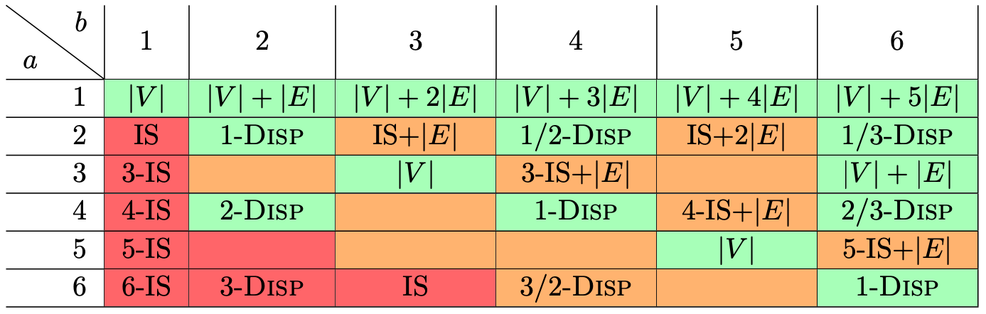
As a first contribution, for every fixed integer $a, b$ , we settle the NP-hardness and the parameterized complexity of finding a maximum $a$ -independent set when parameterized by the solution size (as color-coded in Figure 1). If the ratio $\frac{a}{b}$ is smaller than $2$ , then the problem is FPT, and otherwise it is W[1]-hard unless it is a polynomial time solvable case.

Theorem 1.2 (Section 4).

$a$ - ${\textsc{Independent Set}}(\mathcal{G}_{b})$ is

$\blacksquare$

polynomial time solvable if $b=ca$ or if $b=c\frac{a}{2}$ and $\frac{a}{2}$ is even for some integer $c$ ; and NP-hard for all other integers $a, b$ ; and is
$\blacksquare$

fixed-parameter tractable for the solution size as parameter if $\frac{a}{b}<2$ or if $\frac{a}{b}=2$ , $b$ even; and W[1]-hard for all other integers $a, b$ .

Next, we consider the problem parameterized by treewidth. Intuitively, the $a$ -Independent Set problem is harder for larger $a$ . Indeed, for all $a\geq 2$ , there is a matching upper and lower bound with $a$ in the base of an exponential run time for graphs of bounded treewidth, assuming the Strong Exponential Time Hypothesis (SETH).

Theorem 1.3 (Katsikarelis et al. [20]).

For $a\geq 2$ , given a tree decomposition of width $t$ of an $n$ vertex input graph, a maximum $a$ -independent set can be found in time $a^{t}\cdot{n}^{O(1)}$ . Assuming SETH, there is no $(a-\varepsilon)^{\operatorname{{\mathsf{tw}}}(G)}\cdot n^{O(1)}$ time algorithm for any $\varepsilon>0$ , even for graphs without a cycle of length $<a$ .²²2The restriction to graphs without short cycles is not explicitly given, but easily observed. We will rely on this restriction later.

We refine Theorem 1.3 by restricting the $a$ -Independent Set problem to $b$ -subdivided graphs and determining the optimal base of the exponent for all integers $a$ and $b$ . We expect that larger $a$ makes the problem harder (as in Theorem 1.3) and larger $b$ makes the problem easier (as the graphs become more restricted), but it turns out that the optimal base depends on $a$ and $b$ in a very subtle way. Let $\gcd(a,b)$ denote the greatest common divisor of integers $a$ and $b$ .

Theorem 1.4 (Section 5).

Let $a^{\prime},b^{\prime}$ integers with $\gcd(a^{\prime},b^{\prime})=c$ , $ca=a^{\prime}$ and $cb=b^{\prime}$ . Assume SETH, an $\varepsilon>0$ and that a tree decomposition of width $t$ is part of the input.

$\blacksquare$

If $\gcd(a^{\prime},b^{\prime})$ is odd: If $a=1$ , $a^{\prime}$ - ${\textsc{Independent Set}}(\mathcal{G}_{b^{\prime}})$ is in P, else $a^{\prime}$ - ${\textsc{Independent Set}}(\mathcal{G}_{b^{\prime}})$ can be solved in time $a^{t}\cdot n^{O(1)}$ but not in $(a-\varepsilon)^{\operatorname{{\mathsf{pw}}}(G)}\cdot n^{O(1)}$ .
$\blacksquare$

If $\gcd(a^{\prime},b^{\prime})$ is even: If $a\in\{1,2\}$ , $a^{\prime}$ - ${\textsc{Independent Set}}(\mathcal{G}_{b^{\prime}})$ is in P, else $a^{\prime}$ - ${\textsc{Independent Set}}(\mathcal{G}_{b^{\prime}})$ can be solved in time $(2a)^{t}\cdot n^{O(1)}$ but not in $(2a-\varepsilon)^{\operatorname{{\mathsf{pw}}}(G)}\cdot n^{O(1)}$ .

Refer to caption — Figure 1: Some problems, such as IndependentSet and Dispersion, (or solution sizes) corresponding to $a$ -Independent Set on a graph $G_{b}$ for small values of $a, b$ and $V=V(G)$ and $E=E(G)$ . A light green cell indicates a polynomial time solvable case, an orange NP-hardness & FPT, and a dark red NP-hardness & W[1]-hardness.

The proof heavily uses hidden symmetries of $a$ -independent sets on $b$ -subdivided graphs for different values of $a$ and $b$ . Such symmetries were explored first for a continuous version of $a$ -independent set, in a series of work [14, 17, 15]. We show that these results hold in similar form for $a$ -independent sets as well.

Rational distances.

As the distance between any two vertices in a graph is an integer, it makes no sense to consider $a$ -independent sets for noninteger $a$ . However, noninteger distances can be highly relevant if we consider the complexity of the said continuous version of $a$ -independent. The continuous version, introduced by Dearing and Francis [8], is known as $\delta$ -dispersion for a positive real distance $\delta$ . In this setting, instead of requiring a selection of vertices of a graph $G$ , we allow the selection of points that may be on a vertex or somewhere on the continuum of an edge. We fix the length of the edges to $1$ , which defines a distance relation of the points in the graph $G$ . A $\delta$ -dispersed set then is a subset of points $S$ where every distinct points $p,q\in S$ have distance at least $\delta$ ; as studied for example in [35, 14, 17]. The problem $\delta$ -Dispersion is the decision version asking for a $\delta$ -dispersed set of size at least $k$ , for some budget $k$ given in the input. It turns out that the notion of $\frac{a}{b}$ -dispersed sets is similar to $a$ -independent sets on $b$ -subdivided graphs. Indeed, a crucial connection between the two types of sets is that $\frac{a}{b}$ -dispersed sets are in one-to-one correspondence to $2a$ -independent sets on the $2b$ -subdivided graph, as follows from a discretization argument by Grigoriev et al. [14]. Particularly, the polynomial time solvable case of $a$ -independent set, as stated in Theorem 1.1, follow from this discretization argument and a characterization of the polynomial time solvable cases of $\delta$ -dispersion. Finding a maximum $\delta$ -dispersed set is polynomial time solvable if $\delta$ is a twice a unit-fraction (including $1$ and $2$ ), and all other cases are NP-hard [14]. Further, $\delta$ -dispersion when parameterized by the solution size is FPT when $\delta\leq 2$ and otherwise W[1]-hard, as shown by Hartmann et al. [17].

With such connections and Theorem 1.4 at our hands, we can turn the results on $a$ -independent set on $b$ -subdivided graphs into tight results for $\delta$ -Dispersion on bounded treewidth graphs for every fixed rational $\delta$ .

Theorem 1.5 (Section 5).

Let coprime $a, b$ define $\delta=\frac{a}{b}$ . If $a\leq 2$ , then $\delta$ -Dispersion is in P. For $a\geq 3$ , given a tree decomposition of width $t$ , the problem can be solved in time $(2a)^{t}\cdot n^{O(1)}$ , and, assuming SETH, there is no $(2a-\varepsilon)^{t}\cdot n^{O(1)}$ time algorithm for any $\varepsilon>0$ .

Irrational distances.

By Theorem 1.5, for a fixed rational $\delta=\frac{a}{b}$ , finding a maximum size $\frac{a}{b}$ -dispersed set is fixed-parameter tractable in the treewidth of the input graph. This is not necessarily the case for irrational $\delta$ . Deciding $\delta$ -Dispersion can be as hard as outputting the digits of $\delta$ , which for some $\delta$ is not even computable. Consider, for example, a path of length $\ell$ . Then there is a dispersed set of size $k+1$ if and only if $\frac{\ell}{k}\leq\delta$ . Hence it is reasonable to consider the question of efficient algorithms only if $\delta$ is efficiently comparable to rationals, meaning that there is an algorithm that, given $\frac{y}{x}$ , decides whether $\frac{x}{y}\leq\delta$ in time polynomial in $\log x+\log y$ .

For every fixed efficiently comparable $\delta$ , it is possible to find a maximum $\delta$ -dispersed set in an $n$ -vertex graph in time $n^{O(\operatorname{{\mathsf{tw}}}(G))}$ , i.e., there is an XP algorithm parameterized by treewidth. This follows from a rounding procedure by Hartmann et al. [17], by which for an $n$ -vertex graph the dispersion number of $\delta$ equals to the dispersion number of the smallest rational $\frac{x}{y}$ where $\delta\leq\frac{x}{y}$ with $x\leq 2n$ . Using that $\delta$ is efficiently comparable, we can find this rational in polynomial time since $x\leq 2n$ and $y$ is in the order of $n$ for a fixed $\delta$ . Then it remains to apply the algorithm of Theorem 1.5 to find a maximum $\frac{x}{y}$ -dispersed set.

In contrast, the above algorithm cannot be improved to a fixed-parameter tractable under standard complexity assumptions. As we show, there is a very explicitly defined and efficiently comparable irrational $\delta=(4\sum_{j=1}^{\infty}2^{-2^{j}})^{-1}\approx 0.790085$ , for which computing the $\delta$ -dispersion number is W[1]-hard parameterized by the treewidth (in fact even for pathwidth), and an according lower bound holds under the Exponential Time Hypothesis (ETH).

Theorem 1.6 (Section 6).

There is an efficiently comparable irrational $\delta$ for which $\delta$ -Dispersion is W[1]-hard in the pathwidth $\operatorname{{\mathsf{pw}}}(G)$ of the $n$ -vertex input graph $G$ and, assuming ETH, cannot be solved in time $f(\operatorname{{\mathsf{pw}}}(G))\cdot{n}^{o(\operatorname{{\mathsf{pw}}}(G))}$ for any computable function $f$ .

Domination Problems

In addition to distance $a$ -independent set, we perform a similar study of the dual domination problems. As we show, the results for $a$ -independence hold quite similarly for according domination problems. We use a definition that unifies several concepts such as that of a dominating set and a vertex cover.

A distance- $d$ dominating set $D$ is a subset of vertices such that every other vertex is at distance at most $d$ to a vertex in $D$ . The literature contains several more distance domination-like problems, which are often quite well understood on bounded treewidth graphs. A well-studied example is mixed dominating set, for example [38, 19, 25, 37, 10] and under the name total covering [1, 11, 28, 2, 31], which is (even though not directly phrased as such) equivalent to a distance- $2$ dominating set of the $2$ -subdivision of a graph $G$ . Similarly, a vertex-edge dominating set is a subset of vertices $D$ such that every edge has one of its end vertices in distance at most $1$ to a vertex in $D$ , as studied in [23, 40, 39]. More generally, a distance- $d$ vertex cover (not to be confused with a $d$ -path vertex cover) is a subset of vertices $D$ such that every edge has one of its end vertices in distance at most $d$ to a vertex in $D$ , as studied in [3, 7].

We unify all above concepts by the notion of an ${a}$ -walk dominating set for an integer $a$ , which is a subset of vertices $D$ such that for every edge $e\in E(G)$ , there are (possibly identical) vertices $w_{1},w_{2}\in D$ and a $w_{1},w_{2}$ -walk of length at most $a$ containing edge $e$ .

Observation 1.7.

For a graph $G$ without isolated vertices, the following notions coincide:

$\blacksquare$

a vertex cover and a ${2}$ -walk dominating set,
$\blacksquare$

a dominating set and a ${3}$ -walk dominating set,
$\blacksquare$

a vertex-edge dominating set and a ${4}$ -walk dominating set,
$\blacksquare$

a distance- $d$ dominating set and a ${(2d+1)}$ -walk dominating set, for every $d\geq 1$ ,
$\blacksquare$

a mixed dominating set in $G$ and a ${5}$ -walk dominating set in the $2$ -subdivision $G_{2}$ , and
$\blacksquare$

a distance- $d$ vertex cover and a ${(2d+2)}$ -walk dominating set, for every $d\geq 0$ .

Integer distances.

Finding a minimum ${a}$ -walk dominating set is NP-hard for $a=2$ (i.e., finding minimum vertex cover) and it is not difficult to show that it remains NP-hard for any fixed $a\geq 2$ . In some cases, the hardness also extends to when we restrict the input to $2$ -subdivided graphs: Finding a minimum mixed dominating set, i.e., a ${5}$ -walk dominating set of $2$ -subdivided graphs, is NP-hard, as shown by Majumdar [26]. In contrast, there are polynomial time algorithms for $a\in\{2,4\}$ when the input is a $2$ -subdivided graph.

Theorem 1.8 (Hartmann et al. [18]).

For $a\in\{2,4\}$ , a minimum ${a}$ -walk dominating set on a $2$ -subdivided graph can be found in linear time.³³3 The original statement is about a continuous covering problem, but can be phrased as here by using a discretization argument given in the same work.

These examples give a glimpse into the complexity of finding an ${a}$ -walk dominating set of a $b$ -subdivided graphs for integers $a, b$ . This work settles, for every fixed integer $a, b$ , whether finding a minimum ${a}$ -walk dominating set of a $b$ -subdivided graph is polynomial time solvable or NP-hard, and additionally settles the parameterized complexity for the solution size as parameter (as color-coded in Figure 2). Formally, let $\overline{\gamma}_{a}(G)$ be the minimum cardinality of an ${a}$ -walk dominating set of a graph $G$ . For a graph class $\mathcal{G}$ , let $a$ - $\textsc{Walk Dominating Set}(\mathcal{G})$ be the according decision problem, which is, given a graph $G\in\mathcal{G}$ and an integer $k$ , deciding whether $\overline{\gamma}_{a}(G)\geq k$ .

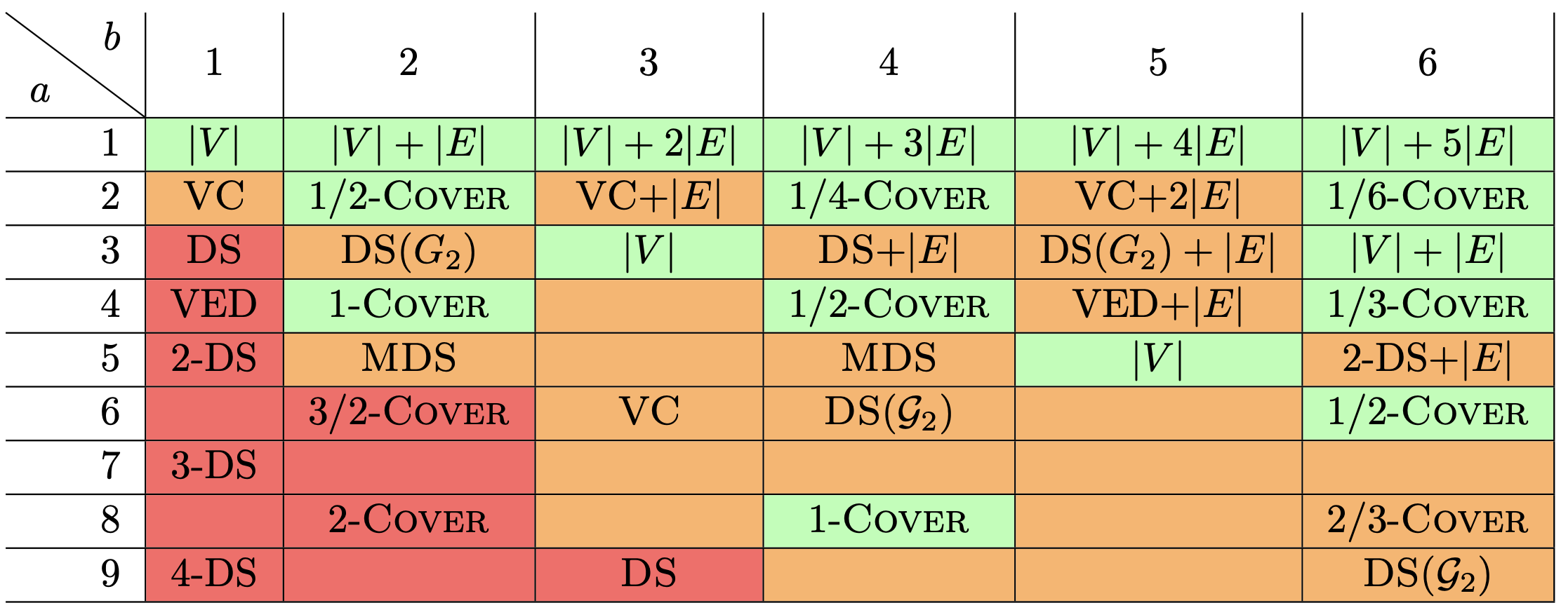
Theorem 1.9 ( ${\star}$ ).

$a$ - $\textsc{Walk Dominating Set}(\mathcal{G}_{b})$ is

$\blacksquare$

polynomial time solvable if $b=ca$ or if $b=c\tfrac{a}{2}$ and $\tfrac{a}{2}$ is even for some integer $c$ ; and is NP-hard for all other integers $a, b$ ; and is
$\blacksquare$

fixed-parameter tractable for the parameter solution size if $\frac{a}{b}<3$ ; and W[2]-hard for all other integers $a, b$ .

We note that $a$ - $\textsc{Walk Dominating Set}(\mathcal{G}_{b})$ is polynomial time solvable for the same set of integers $a, b$ where $a$ - ${\textsc{Independent Set}}(\mathcal{G}_{b})$ is polynomial time solvable. In contrast, the threshold which separates the fixed-parameter tractable cases from the W[1]-hard/W[2]-hard cases is shifted, which should be expected as Vertex Cover and Dominating Set are to be separated by this threshold.

Further, we study the problem parameterized by treewidth. Again, intuitively, the ${a}$ -walk dominating set problem is harder for larger $a$ . Indeed, for many cases the notion of an ${a}$ -walk dominating set corresponds to a known problem (as in 1.7) where the literature knows a matching upper and lower bound with $a$ in the base of an exponential run time for graphs of bounded treewidth, assuming SETH. This is also the case for $a=5$ on $2$ -subdivided graphs, as this corresponds to a mixed dominating set.

Theorem 1.10 ([30, 36, 5, 24, 10]).

For $a\in\{2\}\cup\{3,5,7,\dots\}$ , given a tree decomposition of width $t$ of an $n$ vertex input graph, a minimum ${a}$ -walk dominating set can be found in time $a^{t}\cdot n^{O(1)}$ , and, assuming SETH, there is no $(a-\varepsilon)^{t}\cdot n^{O(1)}$ time algorithm for any $\varepsilon>0$ . Moreover, for $a=5$ this even holds when the input graph is restricted to $2$ -subdivided graphs.

We refine Theorem 1.10 by including also even distances $a\geq 4$ and by considering the restriction of $a$ -Walk Dominating Set to $b$ -subdivided graphs, beyond the case $a=5$ and $b=2$ . We determine the optimal base of the exponent for all integers $a$ and $b$ . As it turns out, the optimal base depends on $a$ and $b$ in a very subtle way.

Theorem 1.11 ( ${\star}$ ).

Let $a^{\prime},b^{\prime}$ integers with $\gcd(a^{\prime},b^{\prime})=c$ and $ca=a^{\prime}$ and $cb=b^{\prime}$ . Assume SETH, $\varepsilon>0$ , and that a tree decomposition of width $t$ is part of the input.

$\blacksquare$

If $\gcd(a^{\prime},b^{\prime})$ is odd: If $a=1$ , $a^{\prime}$ - $\textsc{Walk Dominating Set}(\mathcal{G}_{b^{\prime}})$ is in P, else $a^{\prime}$ - $\textsc{Walk Dominating Set}(\mathcal{G}_{b^{\prime}})$ can be solved in time $a^{t}\cdot n^{O(1)}$ but not in $(a-\varepsilon)^{\operatorname{{\mathsf{pw}}}(G)}\cdot n^{O(1)}$ .
$\blacksquare$

If $\gcd(a^{\prime},b^{\prime})$ is even: If $a\in\{1,2\}$ , $a^{\prime}$ - $\textsc{Walk Dominating Set}(\mathcal{G}_{b^{\prime}})$ is in P, else $a^{\prime}$ - $\textsc{Walk Dominating Set}(\mathcal{G}_{b^{\prime}})$ can be solved in time $(2a)^{t}\cdot n^{O(1)}$ but not $(2a-\varepsilon)^{\operatorname{{\mathsf{pw}}}(G)}\cdot n^{O(1)}$ .

The proof of Theorem 1.11 heavily uses hidden symmetries of ${a}$ -walk dominating sets on $b$ -subdivided graphs, which are of similar nature as for independent sets. Such symmetries were explored first for a continuous version of ${a}$ -walk dominating set [18]. We show that these results hold in similar form for ${a}$ -walk dominating set as well.

Regarding distance- $d$ domination, our results so far imply the following.

Corollary 1.12.

Finding a minimum distance- $d$ dominating set in $b$ -subdivided graphs

$\blacksquare$

is polynomial time solvable if $b$ is a multiple of $2d+1$ , otherwise is NP-hard;
$\blacksquare$

if $b$ is not a multiple of $2d+1$ , with $\gcd(2d+1,b)=c$ can be solved in time $((2d+1)/c)^{t}\cdot n^{O(1)}$ if a tree decomposition of width $t$ is part of the input, and, assuming SETH, cannot be solved in time $((2d+1)/c-\varepsilon)^{\operatorname{{\mathsf{pw}}}(G)}\cdot n^{O(1)}$ ; and
$\blacksquare$

fixed-parameter tractable for the parameter solution size if $\frac{2d+1}{b}<3$ ; and W[2]-hard for all other values of $d, b$ .

Rational distances.

The continuous version of ${a}$ -walk dominating set, as introduced by Shier [33], is known as $\delta$ -covering for a positive real distance $\delta$ . Similarly to $\delta$ -dispersion, we allow the selection of points that may be on a vertex or somewhere on the continuum of an edge. We fix the length of the edges to $1$ , which defines a distance relation of the points in the graph $G$ . A $\delta$ -cover is a set of points $S$ that covers every point $p$ in the graph, that is there is a point $q\in S$ such that $p, q$ have distance at most $\delta$ ; as studied for example in [27, 34] and receiving renewed attention lately [16, 18]. The problem $\delta$ -Covering is the decision version asking for a $\delta$ -cover of size at most $k$ , for some budget $k$ given in the input. The notion of a $\frac{a}{b}$ -cover is quite similar to an ${a}$ -walk dominating set of a $b$ -subdivided graph; though the connection is more subtle compared to the independence problems. Based on a discretization argument by Hartmann et al. [18] we show that $\frac{a}{b}$ -covers are in one-to-one correspondence to ${2a}$ -walk dominating sets on $b$ -subdivided graphs, if $b$ is even; while if $b$ is odd, $\frac{a}{b}$ -covers are in one-to-one correspondence to ${4a}$ -walk dominating sets on $2b$ -subdivided graphs. Particularly, we obtain the polynomial time solvable cases of $\delta$ -covering based on this connection. Finding a minimum $\delta$ -cover is polynomial time solvable if $\delta$ is a unit-fraction and otherwise NP-hard [18]. By the same work, $\delta$ -Covering parameterized by the solution size is FPT in case $\delta<\frac{3}{2}$ an otherwise W[2]-hard. (We observe a similar dichotomy for $a$ -independent sets on $b$ -subdivided graphs, as stated in Theorem 1.9.)

With such connections and Theorem 1.11 at our hands, we can turn the results on $a$ -independent set on $b$ -subdivided graphs into tight results for $\delta$ -Covering on bounded treewidth graphs for every fixed rational $\delta$ .

Theorem 1.13 ( ${\star}$ ).

Let $a^{\prime},b^{\prime}$ integers with $\gcd(a^{\prime},b^{\prime})=c$ and $ca=a^{\prime}$ and $cb=b^{\prime}$ . Assume SETH, $\varepsilon>0$ , and that a tree decomposition of width $t$ is part of the input.

$\blacksquare$

$\frac{a^{\prime}}{b^{\prime}}$ -Covering for $a=1$ is in P; if $a\geq 2$ and $b$ is odd, can be solved in time $(4a)^{t}\cdot n^{O(1)}$ but not in $(4a-\varepsilon)^{\operatorname{{\mathsf{pw}}}(G)}\cdot n^{O(1)}$ ; if $a^{\prime}\geq 2$ and $b$ is even, can be solved in time $(2a)^{t}\cdot n^{O(1)}$ but not in $(2a-\varepsilon)^{\operatorname{{\mathsf{pw}}}(G)}\cdot n^{O(1)}$ .

Irrational distances.

By Theorem 1.13, for every fixed rational $\delta=\frac{a}{b}$ , finding a minimum $\frac{a}{b}$ -cover is fixed-parameter tractable parameterized by the treewidth of the input graph. As is the case for $\delta$ -covering, this is not necessarily true for irrational $\delta$ . Deciding $\delta$ -Covering can be as hard as outputting the digits of $\delta$ , which for some $\delta$ is not even computable. For a path of length $\ell$ , there is a covering set of size $k$ if and only if $\delta\geq\frac{\ell}{2k}$ . Hence it is reasonable to consider only $\delta$ which are efficiently comparable.

For every fixed efficiently comparable $\delta$ , it is possible to find a minimum $\delta$ -cover in time $n^{O(\operatorname{{\mathsf{tw}}}(G))}$ , i.e., there is an XP algorithm parameterized by treewidth. This follows from a rounding procedure by Tamir [34], by which for an $n$ -vertex graph the covering number of $\delta$ equals to the covering number of the largest rational $\frac{x}{y}\leq\delta$ with $x\leq 2n$ . Using that $\delta$ is efficiently comparable, we can find this rational in polynomial time since $x<2n$ and $y$ is in the order of $n$ for a fixed $\delta$ . Then it remains to apply the algorithm of Theorem 1.13 to find a minimum $\frac{x}{y}$ -covering set.

In contrast, the above algorithm cannot be improved to a fixed-parameter tractable under standard complexity assumptions. As we show, there is a very explicitly defined and efficiently comparable irrational $\delta^{\prime}=(2\sum_{j=1}^{\infty}2^{-2^{j}})^{-1}\approx 0.395043$ , for which computing the $\delta^{\prime}$ -covering number is W[1]-hard parameterized by the treewidth (in fact even for pathwidth), and an according lower bound under ETH.

Theorem 1.14 ( ${\star}$ ).

There is an efficiently comparable irrational $\delta^{\prime}$ such that $\delta^{\prime}$ -Covering is W[1]-hard in the pathwidth $\operatorname{{\mathsf{pw}}}(G)$ of the $n$ -vertex input graph $G$ and, assuming ETH, cannot be solved in time $f(\operatorname{{\mathsf{pw}}}(G))\cdot{n}^{o(\operatorname{{\mathsf{pw}}}(G))}$ for any computable function $f$ .

2 Preliminaries

All our graphs are simple and undirected. Usually we assume that our graphs as input do not contain isolated vertices, as they can easily be preprocessed for the studied problems.

$𝒃$ -Subdivision.

For a graph $G$ and an integer $b$ , the $b$ -subdivision of $G$ , denoted as $G_{b}$ , results from $G$ by replacing every edge $\{u,v\}\in E(G)$ by a $u, v$ -path of length $b$ . For example, $G=G_{1}$ . For an edge $\{u,v\}\in E(G)$ and $\beta\in\{0,\dots,b\}$ , let $\text{v}(u,v,\beta)$ be the unique vertex on the unique shortest $u, v$ -path in $G_{b}$ with distance $\beta$ to $u$ and distance $b-\beta$ to $v$ . Let $\mathcal{G}_{b}$ be the class of every graph $H$ that is the $b$ -subdivision $G_{b}$ of a graph $G$ .

Point space.

For a graph $G$ , we assume that its edges have unit length. Let $p(u,v,\lambda)$ , for an edge $\{u,v\}\in E(G)$ and a real $\lambda\in[0,1]$ , denote the point on the edge $\{u,v\}$ with distance $\lambda$ to $u$ and distance $1-\lambda$ to $v$ . Hence $p(u,v,\lambda)$ coincides with $p(u,v,1-\lambda)$ , and the point $p(u,v,0)$ coincides with the vertex $u$ . By $P(G)$ we denote the set of points of a graph $G$ . Let $d(p,q)$ , for two points $p,q\in P(G)$ , denote the distance of $p, q$ of the underlying metric space on $P(G)$ .

Graph parameters.

We use the following well known relation of graph parameters. By $\nu(G)$ we denote the maximum size of a matching in a graph $G$ . A tree decomposition $(T,\beta)$ of $G$ consists of a tree $T$ and a mapping $\beta$ from the vertices of $T$ (referred to as nodes) to subsets of $V(G)$ (referred to as bags), such that (1) $\bigcup_{n\in V(T)}=V(G)$ , (2) $\{u,v\}\in E(G)$ implies a node $n\in V(T)$ with $\{u,v\}\subseteq\beta(n)$ , and (3) for nodes $n_{1},n_{2},n_{3}\in V(T)$ where $n_{2}$ lies on the path from $n_{1}$ to $n_{2}$ , we have $\beta(n_{1})\cap\beta(n_{3})\subseteq\beta(n_{2})$ . The width of a tree decomposition is the maximum of $|\beta(n)|-1$ for all $n\in V(T)$ . A path decomposition of $G$ is a tree decomposition $(P,\beta)$ where $P$ is a path. We let $(\beta(n_{1}),\dots,\beta(n_{t}))$ denote the path decomposition using a path $(n_{1},\dots,n_{t})$ . The treewidth $\operatorname{{\mathsf{tw}}}(G)$ of a graph is the minimum width of a tree decomposition, and likewise the pathwidth $\operatorname{{\mathsf{pw}}}(G)$ is the minimum width of a path decomposition.

It is well known that $2\nu(G)\geq\operatorname{{\mathsf{pw}}}(G)\geq\operatorname{{\mathsf{tw}}}(G)$ . Hence a parameterized algorithm with the treewidth as parameter is more general result than using the pathwidth (assuming a respective decomposition is given in the input). On the other hand, a lower bound for the parameter pathwidth also holds for the parameter treewidth.

Efficiently comparable real.

A real $\delta$ is efficiently comparable if there is an algorithm that, given $\frac{y}{x}$ , decides whether $\frac{x}{y}\leq\delta$ in time polynomial in $\log x+\log y$ .

3 Independent and Dispersed Sets

This section explores the close relationship between $a$ -independent sets and $\delta$ -dispersed sets. Our goal is to establish the following two transformations of $\delta$ -dispersed sets also for independent sets. The first relates the dispersion number to the subdividing the graph.

Lemma 3.1 ([14]).

For every real $\delta>0$ and integer $c\geq 1$ , $\delta\text{-}\mbox{disp}(G)=c\delta\text{-}\mbox{disp}(G_{c})$ .

The second relates the dispersion number of the same graph but of different distances. For certain distances the solution size differs by exactly one point for every edge.

Lemma 3.2 ([17, 15]).

$\delta\text{-}\mbox{disp}(G)+|E(G)|=\tfrac{\delta}{1+\delta}\text{-}\mbox{disp% }(G)$ for every real $\delta>0$ and graph $G$ without cycles of length $<\delta$ .

In a key result later, we will apply Lemma 3.2 multiple time, stated as follows. (The proof thereof and of other statements marked with ${(\star)}$ can be found in the full version of this paper.)

Corollary 3.3 ( ${\star}$ ).

$\delta\text{-}\mbox{disp}(G)=\tfrac{\delta}{1+b\cdot\delta}\text{-}\mbox{disp}% (G)-b|E(G)|$ for an integer $b\geq 1$ , real $\delta>0$ and graph $G$ without cycles of length $<\delta$ .

To obtain Lemma 3.1 and Lemma 3.2 in terms of $a$ -independent sets, we consider certain normalized dispersed sets. To that end, recall that a point $p(u,v,\lambda)\in P(G)$ is $c$ -simple if $\lambda$ is a multiple of $c$ . Further, let $S\subseteq P(G)$ be $c$ -simple if all its points are $c$ -simple. The good news is that there is a direct correspondence of $b$ -simple $\tfrac{a}{b}$ -dispersed sets in a graph $G$ and $a$ -independent sets in the $b$ -subdivision $G_{b}$ .

Observation 3.4.

Let $k\in\mathbb{N}$ . There is an $a$ -independent set of size $k$ in $G_{b}$ , if and only if there is a $b$ -simple $\tfrac{a}{b}$ -dispersed set of size $k$ in $G$ .

Proof.

The vertex $\text{v}(u,v,\beta)$ for an edge $\{u,v\}\in E(G)$ and $\beta\in\{0,\dots,b\}$ corresponds to the $b$ -simple point $p(u,v,\frac{i}{b})$ and vice versa. The distance between vertices corresponds to the same distance of corresponding points multiplied by the factor $\frac{1}{b}$ . $\hfill\blacktriangleleft$

Unfortunately, there may be no minimum $\frac{a}{b}$ -dispersed set that is $b$ -simple. On the positive side, a minimum $\frac{a}{b}$ -dispersed set $S$ can be modified to a $2b$ -simple dispersed set $S^{\star}$ of same size. Actually, one can observe that $S^{\star}$ is not $b$ -simple only because of certain points in $S$ .

Lemma 3.5 ([14]).

For an $\tfrac{a}{b}$ -dispersed set $S$ , the following set $S^{\star}=\{p^{\star}\mid p\in S\}$ is $2b$ -simple and $\tfrac{a}{b}$ -dispersed. For each point $p(u,v,\lambda)$ with $\lambda\in(\tfrac{i}{b}-\tfrac{1}{2b},\tfrac{i}{b}+\tfrac{1}{2b})$ for some integer $i\geq 0$ , let $p^{\star}\coloneqq p(u,v,\tfrac{i}{b})$ ; for all other $p\in S$ , let $p^{\star}=p$ .

Corollary 3.6.

$\tfrac{a}{b}\text{-}\mbox{disp}(G)=\alpha_{2a}(G_{2b})$ for every $a,b\in\mathbb{N}_{+}$ and graph $G$ .

This already implies a subdivision argument almost as for $a$ -independent sets (Lemma 3.1).

Lemma 3.7.

For every graph $G$ , $\alpha_{a}(G_{b})=\alpha_{ca}(G_{cb})$ if $c$ is odd, or $a, b$ are even.

Proof.

First consider that $a$ and $b$ are even. Then $\alpha_{a}(G_{b})=\alpha_{2a^{\prime}}(G_{2b^{\prime}})$ for some integers $a^{\prime},b^{\prime}$ . Then $\alpha_{2a^{\prime}}(G_{2b^{\prime}})=\frac{a^{\prime}}{b^{\prime}}\text{-}% \mbox{disp}=\frac{ca^{\prime}}{cb^{\prime}}\text{-}\mbox{disp}=\alpha_{2ca^{% \prime}}(G_{2cb^{\prime}})=\alpha_{ca}(G_{cb})$ , because of Corollary 3.6.

Now consider that $c$ is odd. Clearly, an $a$ -independent set in $G_{b}$ corresponds to a $c a$ -independent set in $G_{cb}$ . For the reverse direction, let $I\subseteq V(G_{cb})$ be a $c a$ -independent set of $G_{cb}$ . Consider the corresponding $a$ -dispersed set $S\subseteq V(G_{b})$ in $G_{b}$ , which is $b c$ -simple. We apply the construction of Lemma 3.5. As $c$ is odd, there is no point $p\in S$ with edge position $\tfrac{1}{2}$ . Hence the construction only produces points with edge position $0$ or $1$ . That is, the constructed set $S^{\star}$ is $1$ -simple, and hence $S^{\star}$ corresponds to an $a$ -independent set in $G_{b}$ . $\hfill\blacktriangleleft$

Next, we obtain the second connection (Lemma 3.2) quite similarly for dispersed sets. That is, we relate $a$ -independent sets in the subdivided graphs $G_{b}$ and $G_{a+b}$ . The basic idea is to translate the independent set to a dispersed set and apply Lemma 3.2. However, the construction of Lemma 3.2 does not preserve simplicity. Hence we adapt the construction slightly such that it always maps $b$ -simple inputs to $(a+b)$ -simple outputs. As we show in the appendix, the correctness follows with almost the same proof as for Lemma 3.2.

Lemma 3.8 ( ${\star}$ ).

Let $G$ be a graph without a cycle of length $<\tfrac{a}{b}$ . A $b$ -simple $\tfrac{a}{b}$ -dispersed set $S$ implies an $(a+b)$ -simple $\tfrac{a}{a+b}$ -dispersed set of size $|S|+|E(G)|$ . Further, an $(a+b)$ -simple $\tfrac{a}{a+b}$ -dispersed set $S^{\prime}$ implies a $b$ -simple $\tfrac{a}{b}$ -dispersed set of size $|S^{\prime}|-|E(G)|$ .

Equipped with Lemma 3.8, we obtain an result analogous to Lemma 3.2.

Theorem 3.9.

$\alpha_{a}(G_{b})+|E(G)|=\alpha_{a}(G_{a+b})$ if graph $G_{b}$ contains no cycle of length $<a$ .

Proof.

Let $I$ be an $a$ -independent set $I$ in $G_{b}$ . Then $I$ corresponds to a $b$ -simple $\tfrac{a}{b}$ -dispersed set $S$ in $G$ , by 3.4. Lemma 3.8 maps $S$ to an $(a+b)$ -simple $\tfrac{a}{a+b}$ -dispersed set $S^{\prime}$ in $G$ of size $|I|+|E(G)|$ . This construction is applicable since $G_{b}$ contains no cycle of length $<a$ , and hence $G$ contains no cycle of length $<\tfrac{a}{b}$ . Then the $(a+b)$ -simple set $S^{\prime}$ corresponds to an $a$ -independent set in $G_{a+b}$ of size $|I|+|E(G)|$ , by 3.4. That means $\alpha_{a}(G_{b})+|E(G)|\leq\alpha_{a}(G_{a+b})$ .

Vice versa, let $I$ be an $a$ -independent set in $G_{a+b}$ . Then $I^{\prime}$ corresponds to an $(a+b)$ -simple $\tfrac{a}{a+b}$ -dispersed set $S^{\prime}$ in $G$ of size $|I|$ , by 3.4. Lemma 3.8 maps $S$ to an $a$ -simple $\tfrac{a}{b}$ -dispersed set $S$ in $G$ of size $|I^{\prime}|-|E(G)|$ . Then the $b$ -simple set $S$ corresponds to an $a$ -independent set in $G_{b}$ of size $|I^{\prime}|-|E(G)|$ , by 3.4. That means $\alpha_{a}(G_{b})+|E(G)|\geq\alpha_{a}(G_{a+b})$ . $\hfill\blacktriangleleft$

Now with these two relation of independent sets established (Corollary 3.6 and Theorem 3.9), we easily obtain the the integers $a, b$ for which finding a maximum $a$ -independent set on $b$ -subdivided graphs is polynomial time solvable. A simple case is, that $a$ is odd and $b$ is a multiple of $a$ . By Lemma 3.7, this is equivalent to finding a maximum $1$ -independent set on a $\frac{a}{b}$ -subdivided graph, which trivially consist of all vertices. In the case that $a$ is even and $b$ is a multiple of $a$ , and that $\tfrac{a}{2}$ is even and $b$ is a multiple of $\tfrac{a}{2}$ , Lemma 3.7 and Theorem 3.9 allow to reduce the problem to a polynomial time solvable case from Theorem 1.2. Theorem 3.9 is applicable as in above cases $\frac{a}{b}\leq 2$ .

Theorem 3.10.

$a$ -Independent Set on $b$ -subdivided graph is polynomial time solvable if $b$ is a multiple of $a$ , or $\tfrac{a}{2}$ is even and $b$ is an odd multiple of $\tfrac{a}{2}$ .

4 Independent Set with Parameter Solution Size

This section settles the parameterized complexity of finding a maximum $a$ -independent set on $b$ -subdivided graphs with the solution size as parameter, for every integer $a, b$ . These results are also color-coded in Figure 1 and summarized as follows.

Theorem 4.1 (Theorem 1.2 restated).

$a$ - ${\textsc{Independent Set}}(\mathcal{G}_{b})$ is

$\blacksquare$

polynomial time solvable if $b=ca$ or if $b=c\frac{a}{2}$ and $\frac{a}{2}$ is even for some integer $c$ ; and NP-hard for all other integers $a, b$ ; and is
$\blacksquare$

fixed-parameter tractable for the solution size as parameter if $\frac{a}{b}<2$ or if $\frac{a}{b}=2$ , $b$ even; and W[1]-hard for all other integers $a, b$ .

The polynomial time solvable cases are already settled by Theorem 3.10. As is well-known, $2$ -Independent Set (on general graphs, hence $1$ -subdivided graphs) is W[1]-hard [9]. This also puts all cases where $\frac{a}{b}=2$ and $b$ odd to W[1]-hard, by applying Lemma 3.7; while all over cases with $\frac{a}{b}=2$ are polynomial time solvable. The fixed-parameter tractable cases rely on bounding the solution size below by the size of a maximum matching in a graph $G$ , denoted as $\nu(G)$ ; similarly as for the covering problem [17].

Lemma 4.2.

$\nu(G)\leq\alpha_{a}(G_{b})$ for every graph $G$ and integers $a, b$ with $\frac{a}{b}<2$ .

Proof.

If $\frac{a}{b}\leq 1$ , then $V(G)$ is an $a$ -independent set in $G_{b}$ . Since $|V(G)|\geq\nu(G)$ , the statement follows for $\frac{a}{b}\leq 1$ . Otherwise, consider a maximum matching $M\subseteq E(G)$ . Then the two vertices $\text{v}(u,v,\lfloor\frac{b}{2}\rfloor)$ and $\text{v}(u^{\prime},v^{\prime},\lfloor\frac{b}{2}\rfloor)$ for distinct matching edges $\{u,v\},\{u^{\prime},v^{\prime}\}\in M$ have distance at least $b+2\lfloor\frac{b}{2}\rfloor\geq b+({b-1})=2b-1\geq a$ . The last inequality holds since otherwise $2b\leq a$ in contradiction to $\frac{a}{b}<2$ . In conclusion $\{\text{v}(u,v,\lfloor\frac{b}{2}\rfloor)\mid\{u,v\}\in M,u\prec v\}$ is an $a$ -independent set of $G_{b}$ , where $\prec$ is an arbitrary ordering of $V(G)$ . $\hfill\blacktriangleleft$

As the maximum size of a matching in a graph upper bounds the treewidth, an FPT-algorithm results from a win-win situation. Either the input asks for an independent set that is relatively large compared to $\nu(G)$ and hence also compared to the treewidth, in which case we can use Theorem 1.3, or the answer is trivially “yes”.

Lemma 4.3 ( ${\star}$ ).

For every $a, b$ with $\frac{a}{b}<2$ , $a$ - ${\textsc{Independent Set}}(\mathcal{G}_{b})$ is FPT for the parameter solution size.

It remains to show W[1]-hardness if $\frac{a}{b}>2$ , which follows from two parameter preserving reductions from Independent Set showing W[1]-hardness, the first for $\frac{a}{b}\in(2,3)$ , the second for $\frac{a}{b}\geq 3$ ; similarly as for the covering problem [17].

Lemma 4.4 ( ${\star}$ ).

For integers $a, b$ where $\frac{a}{b}>2$ , $a$ - ${\textsc{Independent Set}}(\mathcal{G}_{b})$ is W[1]-hard.

5 Dispersion for Rational Distances

This section derives the upper and lower bounds under SETH for finding a minimum $a$ -independent set on $b$ -subdivided graphs for the parameter treewidth, for all integers $a, b$ . All lower bounds follow from the mere lower bound for even distance $a\geq 6$ .

Theorem 5.1 ( ${\star}$ ).

Let $a\geq 6$ be even. Assuming SETH, $a$ -Independent Set has no $(a-\varepsilon)^{\operatorname{{\mathsf{pw}}}(G)}\cdot n^{O(1)}$ time algorithm for any $\varepsilon>0$ , even when the input is restricted to $2$ -subdivided graphs without a cycle of length $<a$ .

In fact, we show this lower bound assuming the Primal Pathwidth SETH, recently introduced by Lampis [22]. We provide the details in the full version.

Theorem 5.2 (Theorem 1.4, Theorem 1.5 combined).

Let integers $a^{\prime},b^{\prime}$ define $\gcd(a^{\prime},b^{\prime})=c$ and $ca=a^{\prime}$ and $cb=b^{\prime}$ . Assume SETH, an $\varepsilon>0$ and that a tree decomposition of width $t$ is part of the input.

$\blacksquare$

If $\gcd(a^{\prime},b^{\prime})$ is odd: If $a=1$ , $a^{\prime}$ - ${\textsc{Independent Set}}(\mathcal{G}_{b^{\prime}})$ is in P, else $a^{\prime}$ - ${\textsc{Independent Set}}(\mathcal{G}_{b^{\prime}})$ can be solved in time $a^{t}\cdot n^{O(1)}$ but not in $(a-\varepsilon)^{\operatorname{{\mathsf{pw}}}(G)}\cdot n^{O(1)}$ .
$\blacksquare$

If $\gcd(a^{\prime},b^{\prime})$ is even: If $a\in\{1,2\}$ , $a^{\prime}$ - ${\textsc{Independent Set}}(\mathcal{G}_{b^{\prime}})$ is in P, else $a^{\prime}$ - ${\textsc{Independent Set}}(\mathcal{G}_{b^{\prime}})$ can be solved in time $(2a)^{t}\cdot n^{O(1)}$ but not in $(2a-\varepsilon)^{\operatorname{{\mathsf{pw}}}(G)}\cdot n^{O(1)}$ .
$\blacksquare$

If $a^{\prime}\in\{1,2\}$ , $\frac{a^{\prime}}{b^{\prime}}$ -Dispersion is in P; while if $a^{\prime}\geq 3$ can be solved in $(2a)^{t}\cdot n^{O(1)}$ time but not in time $(2a-\varepsilon)^{\operatorname{{\mathsf{pw}}}(G)}\cdot n^{O(1)}$ .

Proof.

First, we consider that $c=\gcd(a^{\prime},b^{\prime})$ is odd. Then $c a$ - ${\textsc{Independent Set}}(\mathcal{G}_{cb})$ is equivalent to $a$ - ${\textsc{Independent Set}}(\mathcal{G}_{b})$ by Lemma 3.7. In case $a=1$ , then $1$ - ${\textsc{Independent Set}}(\mathcal{G}_{b})$ has the trivial $1$ -independent set $|V(G)|$ . Otherwise, $a$ - ${\textsc{Independent Set}}(\mathcal{G}_{b})$ can be solved in time $a^{t}\cdot n^{O(1)}$ using Theorem 1.3.

For the lower bound we use that $yb=1+xa$ for some integers $x, y$ . Assume SETH. Then we know from Theorem 1.3 that $a$ - ${\textsc{Independent Set}}(\mathcal{G}_{1})$ has no $(a-\varepsilon)^{\operatorname{{\mathsf{pw}}}(G)}\cdot n^{O(1)}$ time algorithm for any $\varepsilon>0$ . Particularly, this lower bound relies on graphs without a cycle of length $<a$ . Then Theorem 3.9 applied $x$ times yields that $a$ - ${\textsc{Independent Set}}(\mathcal{G}_{1+xa})$ , and equivalently $a$ - ${\textsc{Independent Set}}(\mathcal{G}_{yb})$ , also has no $(a-\varepsilon)^{\operatorname{{\mathsf{pw}}}(G)}\cdot n^{O(1)}$ time algorithm for any $\varepsilon>0$ . Thus especially $a$ - ${\textsc{Independent Set}}(\mathcal{G}_{b})$ has no $(a-\varepsilon)^{\operatorname{{\mathsf{pw}}}(G)}\cdot n^{O(1)}$ time algorithm. This settles the cases for independent set with odd $\gcd(a^{\prime},b^{\prime})$ .

Next, we consider that $c=\gcd(a^{\prime},b^{\prime})$ is even, hence that $c=2\hat{c}$ for some integer $\hat{c}$ . Then $(2\hat{c}a)$ - ${\textsc{Independent Set}}(\mathcal{G}_{2\hat{c}b})$ is equivalent to $2a$ - ${\textsc{Independent Set}}(\mathcal{G}_{2b})$ , by Lemma 3.7. Again, by Theorem 1.3, $2a$ - ${\textsc{Independent Set}}(\mathcal{G}_{2b})$ can be solved in time $(2a)^{t}\cdot n^{O(1)}$ .

If $a\in\{1,2\}$ , then $a$ -Dispersion is polynomial time solvable, by Theorem 1.1. Further, as $\frac{a}{b}\leq 2$ , applying Lemma 3.2 yields that also $\frac{a^{\prime}}{b^{\prime}}$ -Dispersion is polynomial time solvable (as also observed in [14]). By Corollary 3.6, $2a$ - ${\textsc{Independent Set}}(\mathcal{G}_{2b})$ is equivalent to $\frac{a^{\prime}}{b^{\prime}}$ -Dispersion, hence polynomial time solvable.

In case $a\geq 3$ , and assuming SETH, Theorem 5.1 provides that $2a$ - ${\textsc{Independent Set}}(\mathcal{G}_{2})$ has no $(2a-\varepsilon)^{\operatorname{{\mathsf{pw}}}(G)}\cdot n^{O(1)}$ time algorithm for any $\varepsilon>0$ . Particularly, this lower bound does not rely on graphs with a cycle of length $<a$ . Since $a, b$ are co-prime, again Theorem 3.9 applies, and we obtain that $2a$ - ${\textsc{Independent Set}}(\mathcal{G}_{2b})$ has no $(2a-\varepsilon)^{\operatorname{{\mathsf{pw}}}(G)}\cdot n^{O(1)}$ for any $\varepsilon>0$ . This settles the cases for independent set with even $\gcd(a^{\prime},b^{\prime})$ .

Finally, $\frac{a^{\prime}}{b^{\prime}}$ -Dispersion is equivalent to $\frac{a}{b}$ -Dispersion by definition. Then $\frac{a}{b}$ -Dispersion is equivalent to $2a$ - ${\textsc{Independent Set}}(\mathcal{G}_{2b})$ by Corollary 3.6. Since $a, b$ are co-prime, $2a,2b$ have greatest common devisor $2$ . By the discussion for an greatest common devisor which is even, we follow that $\frac{a}{b}$ -Dispersion has an $(2a)^{t}\cdot n^{O(1)}$ time algorithm, and, assuming SETH, has no $(2a-\varepsilon)^{t}\cdot n^{O(1)}$ time algorithm for any $\varepsilon>0$ . $\hfill\blacktriangleleft$

6 Dispersion for Irrational Distance

This section derives the hardness result for computing a maximum $\delta$ -dispersed set for the efficiently comparable irrational $\delta=(\sum_{j\in[i+1]}2^{2-2^{j}})^{-1}\approx 0.790085$ .

Theorem 6.1 (Theorem 1.6 restated).

There is an efficiently comparable irrational $\delta$ for which $\delta$ -Dispersion is W[1]-hard in the pathwidth $\operatorname{{\mathsf{pw}}}(G)$ of the $n$ -vertex input graph $G$ and, assuming ETH, cannot be solved in time $f(\operatorname{{\mathsf{pw}}}(G))\cdot{n}^{o(\operatorname{{\mathsf{pw}}}(G))}$ for any computable function $f$ .

Figure 3: Reductions used for the proof of Theorem 6.1. Lemma 6.2 is simultaneously a reduction to

c_{i}

-Dispersion and to

(c_{i}-1)

-Dispersion. ’Agnostic’ to whether the distance is

c_{i}

or

c_{i}-1

, Lemma 6.6 reduces to Dispersion with distance

\gamma_{i}

respectively

\delta_{i}

. These rationals

\gamma_{i}

and

\delta_{i}

form an approximation of

\delta

from below and above. Thus the combined reduction reduces to

\delta

-Dispersion.

Our proof is based on two main reductions. The first one is fairly standard: It is a reduction from a colorful clique problem to $c_{i}$ -Dispersion, where $c_{i}=2^{2^{i}}$ is a sufficiently large integer (polynomially bounded in the number of vertices of the colorful clique problem). The reduction is robust in the sense that it is simultaneously a reduction to $(c_{i}-1)$ -Dispersion as well, i.e., the yes/no answer does not change if we reduce the radius by 1. The second reduction is the main nontrivial part of the proof: We reduce $c_{i}$ -Dispersion to $\delta_{i}$ -Dispersion for some rational $\delta_{i}$ in a robust way. That is, the reduction can be interpreted also as a reduction from $(c_{i}-1)$ -Dispersion to $\gamma_{i}$ -Dispersion for some $\gamma_{i}<\delta_{i}$ . Thus if the source instance has the same yes/no answer for radius $c_{i}$ and $c_{i}-1$ , then the target problem has the same answer for any radius $\delta\in[\gamma_{i},\delta_{i}]$ . We manage to define $\gamma_{i},\delta_{i}$ in such a way that there is an irrational $\delta$ that is in $[\gamma_{i},\delta_{i}]$ for every $i$ . Thus for every $i$ , the problem can be reduced to $\delta$ -Dispersion.

Our main tools so far are subdividing (using Lemma 3.1), and translating (using Lemma 3.2). Translating only applies to instances $\langle\delta,G,k\rangle$ where the graph $G$ contains no cycle of length $<\delta$ . Hence, for convenience, let $\textsc{Dispersion}^{\star}$ be the Dispersion problem restricted to instances where the graph $G$ contains no cycle of length $<\delta$ .

The starting point is Colorful Clique where, given a graph $G$ and an integer $k$ and a proper $k$ -coloring of $G$ , the task is to decide whether $G$ contains a $k$ -clique that contains exactly one vertex of each color. It is known [6] that Colorful Clique is W[1]-hard parameterized by the solution size $k$ and, assuming ETH, has no $f(k)\cdot n^{o(k)}$ time algorithm for any computable function $f$ .

The first reduction is based on a reduction from Colorful Clique to the task of finding a maximum $a$ -independent set with $a$ as part of the input, as given by Katsikarelis et al. [20]. We output a graph with enough leeway such that the $\delta$ -dispersion number does not change for $\delta$ in the interval $[c,c-1]$ for some integer $c$ . Doing so, our construction constitutes a reduction from Colorful Clique to $c$ -Dispersion and, at the same time, a reduction from Colorful Clique to $(c-1)$ -Dispersion. Further, we make sure that the construction does not introduce any short cycles.

Lemma 6.2 ( ${\star}$ ).

There is a polynomial time reduction that, given a Colorful Clique-instance $\langle G,k\rangle$ with $k$ color classes of size $n$ , outputs a graph $G^{\prime}$ of pathwidth ${O}(k)$ and integer $k^{\prime}$ , such that: $\langle G,k\rangle$ is a yes-instance of Colorful Clique if and only if $\langle G^{\prime},k^{\prime}\rangle$ is a yes-instance of $32n$ - $\textsc{Dispersion}^{\star}$ if and only if $\langle G^{\prime},k^{\prime}\rangle$ is a yes-instance of $(32n-1)$ - $\textsc{Dispersion}^{\star}$ .

Next, let us define $\delta$ in an abstract sense. Distance $\delta$ is approximated by values $\delta_{i}$ and $\gamma_{i}$ from below and above with increasing precision. The idea is to define distance $\delta_{i}$ by a fraction $\frac{a_{i}}{b_{i}}$ that results from applying translation (Lemma 3.2) and subdivision (Lemma 3.1) to a (quite large) distance $c_{i}$ . Later, our second reduction then reduces to $\delta_{i}$ -Dispersion and to $\gamma_{i}$ -Dispersion by applying the according translation and subdivision.

Definition 6.3.

Let $c_{1},c_{2},\dots\in\mathbb{N}_{+}$ be an increasing integer sequence. Then $a_{0}=b_{0}=1$ and, for $i\geq 1$ ,

a_{i}\coloneqq a_{i-1}c_{i},\quad\quad b_{i}\coloneqq b_{i-1}c_{i}+1,\quad% \quad\delta_{i}\coloneqq\frac{a_{i}}{b_{i}},\quad\quad\gamma_{i}\coloneqq\frac% {a_{i}-a_{i-1}}{b_{i}-b_{i-1}}.

This defines $\delta\coloneqq\lim_{i\to\infty}\delta_{i}$ .

The sequence is decreasing and bounded from below, hence the limit $\delta\coloneqq\lim_{i\to\infty}\delta_{i}$ is well defined.

Lemma 6.4 ( ${\star}$ ).

For $i\geq 2$ , and $\gamma_{i}$ , $\delta$ , $\delta_{i}$ as defined in Definition 6.3, we have $\gamma_{i-1}<\gamma_{i}<\delta<\delta_{i}<\delta_{i-1}$

We obtain nice computational properties if we use the double-exponential sequence for $c_{i}$ .

Lemma 6.5.

Using sequence $c_{i}\coloneqq 2^{2^{i}}$ for Definition 6.3, integers $a_{i},b_{i}$ are polynomial-time computable given $c_{i}$ , and $a_{i}$ is polynomial in $c_{i}$ . Further, $\delta$ is efficiently comparable.

Proof.

We observe that $a_{i}=\prod_{j=1}^{i}c_{j}=2^{2^{1}}\cdot 2^{2^{2}}\cdots 2^{2^{i}}=2^{2^{i+1}% -2}=2^{2^{i+1}}/4={c_{i}}^{2}/4$ , hence that $a_{i}$ is polynomial-time computable given $c_{i}$ and is polynomial in $c_{i}$ . Further, $b_{i}=(\dots((c_{1}+1)c_{2}+1)\dots)c_{i}+1=\sum_{j=1}^{i}c_{j}c_{j+1}\dots c_% {i}\leq i\cdot a_{i}=\log\log c_{i}\cdot c_{i}^{2}/4$ . Hence $b_{i}$ is polynomial-time computable given $c_{i}$ , by at most $2i$ multiplications and additions of integers that are polynomial in $c_{i}$ .

Let us determine $\delta$ . We let $\eta_{i}=\sum_{j=1}^{i}2^{-2^{j}}$ . Then

\textstyle b_{i}\;=\;\sum_{j=1}^{i+1}\;\prod_{k=j}^{i}c_{k}\;=\;\prod_{k=1}^{i% }c_{k}\sum_{j=1}^{i+1}\;\prod_{k=1}^{j-1}c_{k}^{-1}\;=\;a_{i}\sum_{j=1}^{i+1}2% ^{-(2^{j}-2)}\;=\;4a_{i}\eta_{i+1}.

This yields $\delta=\lim_{i\to\infty}\frac{a_{i}}{b_{i}}=\left(4\sum_{j=1}^{\infty}2^{-2^{j% }}\right)^{-1}\approx 0.790085.$

We show that $\delta$ is efficiently comparable, that is there is an algorithm that, given a rational $\frac{x}{y}$ , decides whether $\frac{x}{y}<\delta$ in time polynomial in $\log x+\log y$ . Our algorithm first checks whether $\tfrac{1}{2}<\frac{x}{y}<1$ , and if not can conclude that $\frac{x}{y}<\delta$ or $\frac{x}{y}>\delta$ . Instead of comparing $\frac{x}{y}$ with $\delta$ , we compare their inverses $\frac{y}{x}$ and $\delta^{-1}$ , and output the negated answer. In base $2$ , we obtain that $\delta^{-1}=1.01000100000001\dots$ , which is that the $i$ -th digit $1$ succeeds the $(i-1)$ -st digit $1$ in $2^{i}$ steps. Hence the first $j$ digits (after the dot) of $\delta^{-1}$ can be output in time polynomial in $j$ . We may also output the first $j$ digits (after the dot) of $\frac{y}{x}$ in time polynomial in $j$ . If there is a position where the digits differ, we can conclude whichever is larger. It remains to show that there will be a difference in the first $j=O(\log x+\log y)$ digits of $\delta^{-1}$ and $\frac{y}{x}$ , hence that comparing the first $j$ digits suffices. Indeed, the digits of $\frac{y}{x}$ as a string cannot contain the substring $0^{\lceil\log x\rceil}1$ after the dot. Otherwise $\frac{y}{x}+\frac{y}{x}$ contains the substring $0^{\lceil\log x\rceil-1}1$ after the dot, and by induction $\frac{y}{x}\cdot x=y$ contains the substring $1$ after the dot, in contradiction that $y$ is integer. In contrast, the first $O(\log x)$ digits of $\delta^{-1}$ do include the substring $0^{\lceil\log x\rceil}1$ . Thus it suffices to compare the fist $\log x$ digits of $\delta^{-1}$ and $\frac{y}{x}$ , which concludes the proof. $\hfill\blacktriangleleft$

The following lemma lies at the heart of our result: the definition of the sequences $a_{i}$ , $b_{i}$ , $c_{i}$ allows us to reduce $c_{i}$ -Dispersion to $\delta_{i}$ -Dispersion and, at the same time, $(c_{i}-1)$ -Dispersion to $\gamma_{i}$ -Dispersion with the same reduction.

Lemma 6.6.

Let sequence $(c_{i})_{i\geq 1}$ be as in Definition 6.3. There is a polynomial-time reduction that, given integers $c_{i},k^{\prime}$ and a graph $G^{\prime}$ , outputs a subdivision $G^{\prime\prime}$ of $G^{\prime}$ and integer $k^{\prime\prime}$ , such that: $\langle G^{\prime},k^{\prime}\rangle$ is a yes-instance of $c_{i}$ - $\textsc{Dispersion}^{\star}$ , if and only if the output $\langle G^{\prime\prime},k^{\prime\prime}\rangle$ is a yes-instance of $\delta_{i}$ - $\textsc{Dispersion}^{\star}$ . Also, $\langle G^{\prime},k^{\prime}\rangle$ is a yes-instance of $(c_{i}-1)$ - $\textsc{Dispersion}^{\star}$ , if and only if the output $\langle G^{\prime\prime},k^{\prime\prime}\rangle$ is a yes-instance of $\gamma_{i}$ - $\textsc{Dispersion}^{\star}$ .

Proof.

Let $a_{i},b_{i}$ and sequence $(c_{i})_{i\geq 1}$ be defined as in Definition 6.3. Our algorithm begins by addressing some border cases. If $k^{\prime}=0$ , we output a trivial simultaneous yes-instance of $\delta_{i}$ - $\textsc{Dispersion}^{\star}$ and $\gamma_{i}$ - $\textsc{Dispersion}^{\star}$ . Else, if $c_{i}$ exceeds $|V(G^{\prime})|$ and $k^{\prime}\geq 1$ , we output a trivial simultaneous no-instance. Else, we output an $a_{i-1}$ -subdivision of the input graph $G^{\prime}$ as $G^{\prime\prime}$ and as budget $k^{\prime\prime}=k^{\prime}+b_{i-1}|E(G^{\prime})|$ . Hence $G^{\prime}$ and $G^{\prime\prime}$ have the same pathwidth up to subdividing the edges. Any number of subdivisions of edges may increase the pathwidth only by a total of one. To compute $g_{i}$ with $c_{i}$ as part of the input, we use Lemma 6.5 to compute $a_{i-1}$ and $b_{i-1}$ in polynomial time. In particular, $a_{i-1}$ is polynomial in $c_{i}$ and hence polynomial in $|V(G^{\prime})|$ , such that we may output $G^{\prime\prime}$ , the $a_{i-1}$ -subdivision of $G^{\prime}$ , in polynomial time.

We have $c_{i}\text{-}\mbox{disp}(G^{\prime})=\frac{c_{i}}{1+c_{i}}\text{-}\mbox{disp}(% G^{\prime})-|E(G^{\prime})|$ by Lemma 3.2 and as $G^{\prime}$ contains no cycle of length $<a$ . Applying this translation not only once but $b_{i-1}$ times, by Corollary 3.3, we obtain $c_{i}\text{-}\mbox{disp}(G^{\prime})=\frac{c_{i}}{1+b_{i-1}c_{i}}\text{-}\mbox% {disp}(G^{\prime})-b_{i-1}|E(G^{\prime})|$ . Then by an $a_{i-1}$ -subdivision of the input graph we have $\frac{c_{i}}{1+b_{i-1}c_{i}}\text{-}\mbox{disp}(G^{\prime})=\frac{a_{i-1}c_{i}% }{1+b_{i-1}c_{i}}\text{-}\mbox{disp}(G^{\prime}_{a_{i-1}})=\frac{a_{i}}{b_{i}}% \text{-}\mbox{disp}(G^{\prime\prime})=\delta_{i}\text{-}\mbox{disp}(G^{\prime% \prime})$ by Lemma 3.1. Thus the input $\langle G^{\prime},k^{\prime}\rangle$ is a yes-instance of $c_{i}$ - $\textsc{Dispersion}^{\star}$ , if and only if the output $\langle G^{\prime\prime},k^{\prime\prime}\rangle$ is a yes-instance of $\delta_{i}$ - $\textsc{Dispersion}^{\star}$ .

The analogous transformations yields that $(c_{i}-1)\text{-}\mbox{disp}(G^{\prime})=\frac{a_{i-1}(c_{i}-1)}{1+b_{i-1}(c_{% i}-1)}\text{-}\mbox{disp}(G^{\prime\prime})-b_{i-1}|E(G^{\prime})|$ . We observe that the numerator of the latter is $a_{i-1}(c_{i}-1)=a_{i-1}c_{i}-a_{i-1}=a_{i}-a_{i-1}$ , while the denominator is $1+b_{i-1}(c_{i}-1)=1+b_{i-1}c_{i}-b_{i-1}=b_{i}-b_{i-1}$ . Hence this rational is equal to $\gamma_{i}$ . Thus $\langle G^{\prime},k^{\prime}\rangle$ is a yes-instance of $(c_{i}-1)$ - $\textsc{Dispersion}^{\star}$ , if and only if the output $\langle G^{\prime\prime},k^{\prime\prime}\rangle$ is a yes-instance of $\gamma_{i}$ - $\textsc{Dispersion}^{\star}$ . $\hfill\blacktriangleleft$

Proof of Theorem 6.1.

Let $\delta$ be defined by integer sequence $c_{i}=2^{2^{i}}$ for $i\geq 1$ . Then $\delta$ is efficient comparable by Lemma 6.5. Consider a Colorful Clique-instance $\langle G,k\rangle$ with color classes of size $\hat{n}$ . Let $i$ be such that $\hat{n}\leq c_{i}/32=2^{2^{i}-5}\eqqcolon n$ , hence $32n=c_{i}$ . We note that $c_{j+1}={c^{2}_{j}}$ , for $j\geq 0$ , and hence $n\leq{\hat{n}}^{2}$ . Thus $n$ and $c_{i}$ are polynomial-time computable, and $n,c_{i}$ are polynomial in $\hat{n}$ . We extend the color-classes of $\langle G,k\rangle$ with $n-\hat{n}$ isolated vertices each, resulting in color classes of size $n$ . Next, we apply the reduction of Lemma 6.2 on $\langle G,k\rangle$ , now with $c_{i}$ color classes, which outputs $\langle G^{\prime},k^{\prime}\rangle$ . In turn, we apply the reduction of Lemma 6.6 on $\langle G^{\prime},k^{\prime}\rangle$ which outputs $\langle G^{\prime\prime},k^{\prime\prime}\rangle$ , forming our final output.

We note that the reductions of Lemma 6.2 and Lemma 6.6 are polynomial-time computable. The former outputs a graph of pathwidth ${O}(k)$ , the latter does not change the pathwidth up to a constant. Hence overall we output a graph $G^{\prime\prime}$ of pathwidth ${O}(k)$ .

By Lemma 6.2 and Lemma 6.6, $\langle G,k\rangle$ is a yes-instance of Colorful Clique, if and only if $\langle G^{\prime\prime},k^{\prime\prime}\rangle$ is a yes-instance of $\delta_{i}$ -Dispersion, if and only if $\langle G^{\prime\prime},k^{\prime\prime}\rangle$ is a yes-instance of $\gamma_{i}$ -Dispersion. Since $\gamma_{i}<\delta<\delta_{i}$ , by Lemma 6.4, the dispersion numbers satisfy $\gamma_{i}\text{-}\mbox{disp}(G^{\prime\prime})=\delta\text{-}\mbox{disp}(G^{% \prime\prime})=\delta\text{-}\mbox{disp}(G^{\prime\prime})$ . Thus the output $\langle G^{\prime\prime},k^{\prime\prime}\rangle$ is a yes-instance of $\delta$ -Dispersion, if and only if $\langle G,k\rangle$ is a yes-instance of Colorful Clique.

Since Colorful Clique is W[1]-hard parameterized by $k$ , also $\delta$ -Dispersion is W[1]-hard parameterized by the pathwidth of the input graph. For the lower bound under ETH, assume an $f(\operatorname{{\mathsf{pw}}}(G))\cdot n^{o(\operatorname{{\mathsf{pw}}}(G))}$ time algorithm for $\delta$ -Dispersion for a computable function $f$ . Then using the above reduction on a Colorful Clique-instance yields an $f(k)\cdot n^{o(k)}$ time algorithm for Colorful Clique, in contradiction to ETH. $\hfill\blacktriangleleft$

7 Domination and Covering

Finally, we turn to the domination problems and covering as their continuous counterpart. This section outlines the connection of ${a}$ -walk dominating set and $\delta$ -covers. We establish tools that relate ${a}$ -walk dominating set on $b$ -subdivided graphs for different values of $a, b$ , similarly as we did for the independent set problem. These tools then allow to derive the complexity results for $a$ -Walk Dominating Set on $b$ -subdivided graphs and $\delta$ -Covering as stated in the introduction. The details thereof are deferred to the full version.

The notion of an ${a}$ -walk dominating set can be defined in three different ways, (D1), (D2) and (D3), which are useful for different kind of proofs. Let $G$ be a graph without isolated vertices. For an integer $a$ , a subset $D\subseteq V(G)$ $a$ -walk dominates some subset of edges $E^{\prime}\subseteq E(G)$ , defining $V^{\prime}\coloneqq V(G[E^{\prime}])$ , if:

$\blacksquare$

$($ D1 $)$ For every edge $e\in E^{\prime}$ , there are (possibly identical) vertices $w_{1},w_{2}\in D$ and a $w_{1},w_{2}$ -walk in $G$ of length at most $a$ that contains $e$ ; or
$\blacksquare$

$($ D2 $)$ Every vertex $u\in V(G[E^{\prime}])$ has $d(u,D)\leq\tfrac{a}{2}$ , and the set vertices $u\in V(G[E^{\prime}])$ where $d(u,D)=\tfrac{a}{2}$ forms an independent set.
$\blacksquare$

$($ D3 $)$ $D\subseteq V(G)$ $a$ -dominates $V^{\prime}\cup E^{\prime}$ in the $2$ -subdivision $G_{2}$ of $G$ (when identifiying an edge $\{u,v\}$ with the vertex with neighborhood $\{u,v\}$ in $G_{2}$ ). That is, for every vertex $u\in V^{\prime}\cup E^{\prime}$ , there is a vertex $w\in D$ with $d_{G_{2}}(u,w)\leq a$ .

An $a$ -walk dominating set of $G$ is a subset $D\subseteq V(G)$ that $a$ -walk dominates $E(G)$ .

Lemma 7.1 ( ${\star}$ ).

Conditions (D1), (D2), (D3) are equivalent.

We have the following two transformation of $\delta$ -dispersed sets for different values of $\delta$ , as shown by Hartmann et al. [18].

Lemma 7.2 ([18]).

For every real $\delta>0$ and integer $c\geq 1$ , $\delta\text{-}\mbox{cover}(G)=c\delta\text{-}\mbox{cover}(G_{c})$ .

Lemma 7.3 ([18]).

$\delta\text{-}\mbox{cover}(G)+|E(G)|=\tfrac{\delta}{1+2\delta}\text{-}\mbox{% cover}(G)$ .

Aiming to translate these modifications to the realm of ${a}$ -walk dominating set on $b$ -subdivided graphs, we observe the following connection.

Observation 7.4 ( ${\star}$ ).

Let $k\in\mathbb{N}$ . There is a $b$ -simple $\tfrac{a}{2b}$ -covering set of size $k$ of a graph $G$ without isolated vertices, if and only if there is an ${a}$ -walk dominating set of $G_{b}$ of size $k$ .

A minimum $\tfrac{a}{b}$ -cover $S$ can be assumed to be $b$ -simple [18]. Actually, if $b$ is even, we observation can be improved. For example, a $\tfrac{1}{2}$ -covering set implies a $2$ -simple $\tfrac{1}{2}$ -covering set of same size.

Lemma 7.5 ( ${\star}$ ).

Let $S$ be an $\tfrac{a}{b}$ -cover of a graph $G$ for integers $a,b\in\mathbb{N}$ . Then there is an $\tfrac{a}{b}$ -cover $S^{\star}$ of $G$ of size $|S^{\star}|=|S|$ that is $2b$ -simple and, if $b$ is a multiple of $2$ , is $b$ -simple.

Assuming that $S$ contains no point at a position $\tfrac{2i-1}{2b}$ for $i\in\mathbb{N}$ , then $S^{\star}$ is $b$ -simple, and, if additionally $b$ is a multiple of $2$ , $S^{\star}$ is $\frac{b}{2}$ -simple.

With this connection at hand, we can state a refined connection of minimum $\frac{a}{b}$ -covers of a graph $G$ and minimum ${a}$ -walk dominating set on $b$ -subdivided graphs.

Corollary 7.6.

$\tfrac{a}{b}\text{-}\mbox{cover}(G)=\overline{\gamma}_{4a}(G_{2b})=\overline{% \gamma}_{4ca}(G_{2cb})$ ; $\tfrac{a}{2b}\text{-}\mbox{cover}(G)=\overline{\gamma}_{2a}(G_{2b})=\overline{% \gamma}_{2ca}(G_{2cb})$ , for any $a,b,c\in\mathbb{N}$ and graph $G$ without isolated vertices.

Now we can put the earlier stated transformation of $\delta$ -dispersed sets in terms of ${a}$ -walk dominating on $b$ -subdivided graphs.

Theorem 7.7 ( ${\star}$ ).

$\overline{\gamma}_{a}(G_{b})=\overline{\gamma}_{ca}(G_{cb})$ when $c$ is odd, or $a, b$ are even.

Theorem 7.8 ( ${\star}$ ).

$\overline{\gamma}_{a}(G_{b})+|E(G)|=\overline{\gamma}_{a}(G_{a+b})$ .

These two transformation lay the groundwork for show Theorem 1.11, Theorem 1.13 and Theorem 1.14. For details, we refer to the full version.

References

[1] Yousef Alavi, M. Behzad, Linda M. Lesniak-Foster, and E. A. Nordhaus. Total matchings and total coverings of graphs. Journal of Graph Theory, 1(2):135–140, 1977. doi:10.1002/jgt.3190010209.
[2] Yousef Alavi, Jiuqiang Liu, Jianfang Wang, and Zhongfu Zhang. On total covers of graphs. Discret. Math., 100(1-3):229–233, 1992. doi:10.1016/0012-365X(92)90643-T.
[3] José D. Alvarado, Simone Dantas, and Dieter Rautenbach. Distance k-domination, distance k-guarding, and distance k-vertex cover of maximal outerplanar graphs. Discret. Appl. Math., 194:154–159, 2015. doi:10.1016/J.DAM.2015.05.010.
[4] Gábor Bacsó, Daniel Lokshtanov, Dániel Marx, Marcin Pilipczuk, Zsolt Tuza, and Erik Jan Van Leeuwen. Subexponential-time algorithms for maximum independent set in $P_{t}$ -free and broom-free graphs. Algorithmica, 81:421–438, 2019.
[5] Glencora Borradaile and Hung Le. Optimal dynamic program for r-domination problems over tree decompositions. In Jiong Guo and Danny Hermelin, editors, 11th International Symposium on Parameterized and Exact Computation, IPEC 2016, August 24-26, 2016, Aarhus, Denmark, volume 63 of LIPIcs, pages 8:1–8:23. Schloss Dagstuhl – Leibniz-Zentrum für Informatik, 2016. doi:10.4230/LIPIcs.IPEC.2016.8.
[6] Marek Cygan, Fedor V. Fomin, Lukasz Kowalik, Daniel Lokshtanov, Dániel Marx, Marcin Pilipczuk, Michal Pilipczuk, and Saket Saurabh. Parameterized Algorithms. Springer, 2015. doi:10.1007/978-3-319-21275-3.
[7] Clément Dallard, Mirza Krbezlija, and Martin Milanic. Vertex cover at distance on H-free graphs. In Paola Flocchini and Lucia Moura, editors, Combinatorial Algorithms – 32nd International Workshop, IWOCA 2021, Ottawa, ON, Canada, July 5-7, 2021, Proceedings, volume 12757 of Lecture Notes in Computer Science, pages 237–251. Springer, 2021. doi:10.1007/978-3-030-79987-8_17.
[8] Perino M. Dearing and Richard L. Francis. A minimax location problem on a network. Transportation Science, 8(4):333–343, 1974.
[9] Rodney G. Downey and Michael R. Fellows. Fixed-parameter tractability and completeness II: on completeness for W[1]. Theor. Comput. Sci., 141(1&2):109–131, 1995. doi:10.1016/0304-3975(94)00097-3.
[10] Louis Dublois, Michael Lampis, and Vangelis T. Paschos. New algorithms for mixed dominating set. Discret. Math. Theor. Comput. Sci., 23(1), 2021. doi:10.46298/DMTCS.6824.
[11] Paul Erdős and Amram Meir. On total matching numbers and total covering numbers of complementary graphs. Discret. Math., 19(3):229–233, 1977. doi:10.1016/0012-365X(77)90102-9.
[12] Hiroshi Eto, Fengrui Guo, and Eiji Miyano. Distance- $d$ independent set problems for bipartite and chordal graphs. J. Comb. Optim., 27(1):88–99, 2014. doi:10.1007/s10878-012-9594-4.
[13] Hiroshi Eto, Takehiro Ito, Zhilong Liu, and Eiji Miyano. Approximation algorithm for the distance-3 independent set problem on cubic graphs. In Sheung-Hung Poon, Md. Saidur Rahman, and Hsu-Chun Yen, editors, WALCOM: Algorithms and Computation, 11th International Conference and Workshops, WALCOM 2017, Hsinchu, Taiwan, March 29-31, 2017, Proceedings, volume 10167 of Lecture Notes in Computer Science, pages 228–240. Springer, 2017. doi:10.1007/978-3-319-53925-6_18.
[14] Alexander Grigoriev, Tim A. Hartmann, Stefan Lendl, and Gerhard J. Woeginger. Dispersing obnoxious facilities on a graph. Algorithmica, 83(6):1734–1749, 2021. doi:10.1007/s00453-021-00800-3.
[15] Tim A. Hartmann. Facility location on graphs. Dissertation, RWTH Aachen University, Aachen, 2022. doi:10.18154/RWTH-2023-01837.
[16] Tim A. Hartmann and Tom Janßen. Approximating $\delta$ -covering (to appear). In Approximation and Online Algorithms – 22nd International Workshop, WAOA 2024, Egham, United Kingdom, September 5-6, 2024, Proceedings, Lecture Notes in Computer Science. Springer, 2024.
[17] Tim A. Hartmann and Stefan Lendl. Dispersing obnoxious facilities on graphs by rounding distances. In Stefan Szeider, Robert Ganian, and Alexandra Silva, editors, 47th International Symposium on Mathematical Foundations of Computer Science, MFCS 2022, August 22-26, 2022, Vienna, Austria, volume 241 of LIPIcs, pages 55:1–55:14. Schloss Dagstuhl – Leibniz-Zentrum für Informatik, 2022. doi:10.4230/LIPICS.MFCS.2022.55.
[18] Tim A. Hartmann, Stefan Lendl, and Gerhard J. Woeginger. Continuous facility location on graphs. Math. Program., 192(1):207–227, 2022. doi:10.1007/s10107-021-01646-x.
[19] Pallavi Jain, Jayakrishnan Madathil, Fahad Panolan, and Abhishek Sahu. Mixed dominating set: A parameterized perspective. In Hans L. Bodlaender and Gerhard J. Woeginger, editors, Graph-Theoretic Concepts in Computer Science – 43rd International Workshop, WG 2017, Eindhoven, The Netherlands, June 21-23, 2017, Revised Selected Papers, volume 10520 of Lecture Notes in Computer Science, pages 330–343. Springer, 2017. doi:10.1007/978-3-319-68705-6_25.
[20] Ioannis Katsikarelis, Michael Lampis, and Vangelis T. Paschos. Structurally parameterized d-scattered set. Discret. Appl. Math., 308:168–186, 2022. doi:10.1016/j.dam.2020.03.052.
[21] Ioannis Katsikarelis, Michael Lampis, and Vangelis T. Paschos. Improved (in-)approximability bounds for d-scattered set. J. Graph Algorithms Appl., 27(3):219–238, 2023. doi:10.7155/JGAA.00621.
[22] Michael Lampis. The primal pathwidth SETH. CoRR, abs/2403.07239, 2024. doi:10.48550/arXiv.2403.07239.
[23] Jason Lewis, Stephen T. Hedetniemi, Teresa W. Haynes, and Gerd H. Fricke. Vertex-edge domination. Utilitas mathematica, 81:193–213, 2010.
[24] Daniel Lokshtanov, Dániel Marx, and Saket Saurabh. Known algorithms on graphs of bounded treewidth are probably optimal. ACM Trans. Algorithms, 14(2):13:1–13:30, 2018. doi:10.1145/3170442.
[25] Jayakrishnan Madathil, Fahad Panolan, Abhishek Sahu, and Saket Saurabh. On the complexity of mixed dominating set. In René van Bevern and Gregory Kucherov, editors, Computer Science – Theory and Applications – 14th International Computer Science Symposium in Russia, CSR 2019, Novosibirsk, Russia, July 1-5, 2019, Proceedings, volume 11532 of Lecture Notes in Computer Science, pages 262–274. Springer, 2019. doi:10.1007/978-3-030-19955-5_23.
[26] Aniket Majumdar. Neighborhood hypergraphs: A framework for covering and packing parameters in graphs. Dissertation, Clemson University, 1992.
[27] Nimrod Megiddo and Arie Tamir. New results on the complexity of $p$ -center problems. SIAM J. Comput., 12(4):751–758, 1983. doi:10.1137/0212051.
[28] Amram Meir. On total covering and matching of graphs. J. Comb. Theory B, 24(2):164–168, 1978. doi:10.1016/0095-8956(78)90017-5.
[29] Pedro Montealegre and Ioan Todinca. On distance-d independent set and other problems in graphs with “few” minimal separators. In Pinar Heggernes, editor, Graph-Theoretic Concepts in Computer Science – 42nd International Workshop, WG 2016, Istanbul, Turkey, June 22-24, 2016, Revised Selected Papers, volume 9941 of Lecture Notes in Computer Science, pages 183–194, 2016. doi:10.1007/978-3-662-53536-3_16.
[30] Rolf Niedermeier. Invitation to Fixed-Parameter Algorithms. Oxford University Press, 2006. doi:10.1093/ACPROF:OSO/9780198566076.001.0001.
[31] Uri N. Peled and Feng Sun. Total matchings and total coverings of threshold graphs. Discret. Appl. Math., 49(1-3):325–330, 1994. doi:10.1016/0166-218X(94)90216-X.
[32] Michal Pilipczuk and Sebastian Siebertz. Kernelization and approximation of distance-r independent sets on nowhere dense graphs. Eur. J. Comb., 94:103309, 2021. doi:10.1016/J.EJC.2021.103309.
[33] Douglas R. Shier. A min-max theorem for $p$ -center problems on a tree. Transportation Science, 11(3):243–252, 1977. URL: http://www.jstor.org/stable/25767877.
[34] Arie Tamir. On the solution value of the continuous ${p}$ -center location problem on a graph. Math. Oper. Res., 12(2):340–349, 1987. doi:10.1287/moor.12.2.340.
[35] Arie Tamir. Obnoxious facility location on graphs. SIAM J. Discret. Math., 4(4):550–567, 1991. doi:10.1137/0404048.
[36] Johan M. M. van Rooij, Hans L. Bodlaender, and Peter Rossmanith. Dynamic programming on tree decompositions using generalised fast subset convolution. In Amos Fiat and Peter Sanders, editors, Algorithms – ESA 2009, 17th Annual European Symposium, Copenhagen, Denmark, September 7-9, 2009. Proceedings, volume 5757 of Lecture Notes in Computer Science, pages 566–577. Springer, 2009. doi:10.1007/978-3-642-04128-0_51.
[37] Mingyu Xiao and Zimo Sheng. Improved parameterized algorithms and kernels for mixed domination. Theor. Comput. Sci., 815:109–120, 2020. doi:10.1016/J.TCS.2020.02.014.
[38] Yancai Zhao, Liying Kang, and Moo Young Sohn. The algorithmic complexity of mixed domination in graphs. Theor. Comput. Sci., 412(22):2387–2392, 2011. doi:10.1016/J.TCS.2011.01.029.
[39] Radosław Ziemann and Paweł Żyliński. Vertex-edge domination in cubic graphs. Discret. Math., 343(11):112075, 2020. doi:10.1016/J.DISC.2020.112075.
[40] Paweł Żyliński. Vertex-edge domination in graphs. Aequationes mathematicae, 93(4):735–742, 2019.

[bib.bib1] [1] Yousef Alavi, M. Behzad, Linda M. Lesniak-Foster, and E. A. Nordhaus. Total matchings and total coverings of graphs. Journal of Graph Theory, 1(2):135–140, 1977. doi:10.1002/jgt.3190010209.

[bib.bib2] [2] Yousef Alavi, Jiuqiang Liu, Jianfang Wang, and Zhongfu Zhang. On total covers of graphs. Discret. Math., 100(1-3):229–233, 1992. doi:10.1016/0012-365X(92)90643-T.

[bib.bib3] [3] José D. Alvarado, Simone Dantas, and Dieter Rautenbach. Distance k-domination, distance k-guarding, and distance k-vertex cover of maximal outerplanar graphs. Discret. Appl. Math., 194:154–159, 2015. doi:10.1016/J.DAM.2015.05.010.

[bib.bib4] [4] Gábor Bacsó, Daniel Lokshtanov, Dániel Marx, Marcin Pilipczuk, Zsolt Tuza, and Erik Jan Van Leeuwen. Subexponential-time algorithms for maximum independent set in $P_{t}$ -free and broom-free graphs. Algorithmica, 81:421–438, 2019.

[bib.bib5] [5] Glencora Borradaile and Hung Le. Optimal dynamic program for r-domination problems over tree decompositions. In Jiong Guo and Danny Hermelin, editors, 11th International Symposium on Parameterized and Exact Computation, IPEC 2016, August 24-26, 2016, Aarhus, Denmark, volume 63 of LIPIcs, pages 8:1–8:23. Schloss Dagstuhl – Leibniz-Zentrum für Informatik, 2016. doi:10.4230/LIPIcs.IPEC.2016.8.

[bib.bib6] [6] Marek Cygan, Fedor V. Fomin, Lukasz Kowalik, Daniel Lokshtanov, Dániel Marx, Marcin Pilipczuk, Michal Pilipczuk, and Saket Saurabh. Parameterized Algorithms. Springer, 2015. doi:10.1007/978-3-319-21275-3.

[bib.bib7] [7] Clément Dallard, Mirza Krbezlija, and Martin Milanic. Vertex cover at distance on H-free graphs. In Paola Flocchini and Lucia Moura, editors, Combinatorial Algorithms – 32nd International Workshop, IWOCA 2021, Ottawa, ON, Canada, July 5-7, 2021, Proceedings, volume 12757 of Lecture Notes in Computer Science, pages 237–251. Springer, 2021. doi:10.1007/978-3-030-79987-8_17.

[bib.bib8] [8] Perino M. Dearing and Richard L. Francis. A minimax location problem on a network. Transportation Science, 8(4):333–343, 1974.

[bib.bib9] [9] Rodney G. Downey and Michael R. Fellows. Fixed-parameter tractability and completeness II: on completeness for W[1]. Theor. Comput. Sci., 141(1&2):109–131, 1995. doi:10.1016/0304-3975(94)00097-3.

[bib.bib10] [10] Louis Dublois, Michael Lampis, and Vangelis T. Paschos. New algorithms for mixed dominating set. Discret. Math. Theor. Comput. Sci., 23(1), 2021. doi:10.46298/DMTCS.6824.

[bib.bib11] [11] Paul Erdős and Amram Meir. On total matching numbers and total covering numbers of complementary graphs. Discret. Math., 19(3):229–233, 1977. doi:10.1016/0012-365X(77)90102-9.

[bib.bib12] [12] Hiroshi Eto, Fengrui Guo, and Eiji Miyano. Distance- $d$ independent set problems for bipartite and chordal graphs. J. Comb. Optim., 27(1):88–99, 2014. doi:10.1007/s10878-012-9594-4.

[bib.bib13] [13] Hiroshi Eto, Takehiro Ito, Zhilong Liu, and Eiji Miyano. Approximation algorithm for the distance-3 independent set problem on cubic graphs. In Sheung-Hung Poon, Md. Saidur Rahman, and Hsu-Chun Yen, editors, WALCOM: Algorithms and Computation, 11th International Conference and Workshops, WALCOM 2017, Hsinchu, Taiwan, March 29-31, 2017, Proceedings, volume 10167 of Lecture Notes in Computer Science, pages 228–240. Springer, 2017. doi:10.1007/978-3-319-53925-6_18.

[bib.bib14] [14] Alexander Grigoriev, Tim A. Hartmann, Stefan Lendl, and Gerhard J. Woeginger. Dispersing obnoxious facilities on a graph. Algorithmica, 83(6):1734–1749, 2021. doi:10.1007/s00453-021-00800-3.

[bib.bib15] [15] Tim A. Hartmann. Facility location on graphs. Dissertation, RWTH Aachen University, Aachen, 2022. doi:10.18154/RWTH-2023-01837.

[bib.bib16] [16] Tim A. Hartmann and Tom Janßen. Approximating $\delta$ -covering (to appear). In Approximation and Online Algorithms – 22nd International Workshop, WAOA 2024, Egham, United Kingdom, September 5-6, 2024, Proceedings, Lecture Notes in Computer Science. Springer, 2024.

[bib.bib17] [17] Tim A. Hartmann and Stefan Lendl. Dispersing obnoxious facilities on graphs by rounding distances. In Stefan Szeider, Robert Ganian, and Alexandra Silva, editors, 47th International Symposium on Mathematical Foundations of Computer Science, MFCS 2022, August 22-26, 2022, Vienna, Austria, volume 241 of LIPIcs, pages 55:1–55:14. Schloss Dagstuhl – Leibniz-Zentrum für Informatik, 2022. doi:10.4230/LIPICS.MFCS.2022.55.

[bib.bib18] [18] Tim A. Hartmann, Stefan Lendl, and Gerhard J. Woeginger. Continuous facility location on graphs. Math. Program., 192(1):207–227, 2022. doi:10.1007/s10107-021-01646-x.

[bib.bib19] [19] Pallavi Jain, Jayakrishnan Madathil, Fahad Panolan, and Abhishek Sahu. Mixed dominating set: A parameterized perspective. In Hans L. Bodlaender and Gerhard J. Woeginger, editors, Graph-Theoretic Concepts in Computer Science – 43rd International Workshop, WG 2017, Eindhoven, The Netherlands, June 21-23, 2017, Revised Selected Papers, volume 10520 of Lecture Notes in Computer Science, pages 330–343. Springer, 2017. doi:10.1007/978-3-319-68705-6_25.

[bib.bib20] [20] Ioannis Katsikarelis, Michael Lampis, and Vangelis T. Paschos. Structurally parameterized d-scattered set. Discret. Appl. Math., 308:168–186, 2022. doi:10.1016/j.dam.2020.03.052.

[bib.bib21] [21] Ioannis Katsikarelis, Michael Lampis, and Vangelis T. Paschos. Improved (in-)approximability bounds for d-scattered set. J. Graph Algorithms Appl., 27(3):219–238, 2023. doi:10.7155/JGAA.00621.

[bib.bib22] [22] Michael Lampis. The primal pathwidth SETH. CoRR, abs/2403.07239, 2024. doi:10.48550/arXiv.2403.07239.

[bib.bib23] [23] Jason Lewis, Stephen T. Hedetniemi, Teresa W. Haynes, and Gerd H. Fricke. Vertex-edge domination. Utilitas mathematica, 81:193–213, 2010.

[bib.bib24] [24] Daniel Lokshtanov, Dániel Marx, and Saket Saurabh. Known algorithms on graphs of bounded treewidth are probably optimal. ACM Trans. Algorithms, 14(2):13:1–13:30, 2018. doi:10.1145/3170442.

[bib.bib25] [25] Jayakrishnan Madathil, Fahad Panolan, Abhishek Sahu, and Saket Saurabh. On the complexity of mixed dominating set. In René van Bevern and Gregory Kucherov, editors, Computer Science – Theory and Applications – 14th International Computer Science Symposium in Russia, CSR 2019, Novosibirsk, Russia, July 1-5, 2019, Proceedings, volume 11532 of Lecture Notes in Computer Science, pages 262–274. Springer, 2019. doi:10.1007/978-3-030-19955-5_23.

[bib.bib26] [26] Aniket Majumdar. Neighborhood hypergraphs: A framework for covering and packing parameters in graphs. Dissertation, Clemson University, 1992.

[bib.bib27] [27] Nimrod Megiddo and Arie Tamir. New results on the complexity of $p$ -center problems. SIAM J. Comput., 12(4):751–758, 1983. doi:10.1137/0212051.

[bib.bib28] [28] Amram Meir. On total covering and matching of graphs. J. Comb. Theory B, 24(2):164–168, 1978. doi:10.1016/0095-8956(78)90017-5.

[bib.bib29] [29] Pedro Montealegre and Ioan Todinca. On distance-d independent set and other problems in graphs with “few” minimal separators. In Pinar Heggernes, editor, Graph-Theoretic Concepts in Computer Science – 42nd International Workshop, WG 2016, Istanbul, Turkey, June 22-24, 2016, Revised Selected Papers, volume 9941 of Lecture Notes in Computer Science, pages 183–194, 2016. doi:10.1007/978-3-662-53536-3_16.

[bib.bib30] [30] Rolf Niedermeier. Invitation to Fixed-Parameter Algorithms. Oxford University Press, 2006. doi:10.1093/ACPROF:OSO/9780198566076.001.0001.

[bib.bib31] [31] Uri N. Peled and Feng Sun. Total matchings and total coverings of threshold graphs. Discret. Appl. Math., 49(1-3):325–330, 1994. doi:10.1016/0166-218X(94)90216-X.

[bib.bib32] [32] Michal Pilipczuk and Sebastian Siebertz. Kernelization and approximation of distance-r independent sets on nowhere dense graphs. Eur. J. Comb., 94:103309, 2021. doi:10.1016/J.EJC.2021.103309.

[bib.bib33] [33] Douglas R. Shier. A min-max theorem for $p$ -center problems on a tree. Transportation Science, 11(3):243–252, 1977. URL: http://www.jstor.org/stable/25767877.

[bib.bib34] [34] Arie Tamir. On the solution value of the continuous ${p}$ -center location problem on a graph. Math. Oper. Res., 12(2):340–349, 1987. doi:10.1287/moor.12.2.340.

[bib.bib35] [35] Arie Tamir. Obnoxious facility location on graphs. SIAM J. Discret. Math., 4(4):550–567, 1991. doi:10.1137/0404048.

[bib.bib36] [36] Johan M. M. van Rooij, Hans L. Bodlaender, and Peter Rossmanith. Dynamic programming on tree decompositions using generalised fast subset convolution. In Amos Fiat and Peter Sanders, editors, Algorithms – ESA 2009, 17th Annual European Symposium, Copenhagen, Denmark, September 7-9, 2009. Proceedings, volume 5757 of Lecture Notes in Computer Science, pages 566–577. Springer, 2009. doi:10.1007/978-3-642-04128-0_51.

[bib.bib37] [37] Mingyu Xiao and Zimo Sheng. Improved parameterized algorithms and kernels for mixed domination. Theor. Comput. Sci., 815:109–120, 2020. doi:10.1016/J.TCS.2020.02.014.

[bib.bib38] [38] Yancai Zhao, Liying Kang, and Moo Young Sohn. The algorithmic complexity of mixed domination in graphs. Theor. Comput. Sci., 412(22):2387–2392, 2011. doi:10.1016/J.TCS.2011.01.029.

[bib.bib39] [39] Radosław Ziemann and Paweł Żyliński. Vertex-edge domination in cubic graphs. Discret. Math., 343(11):112075, 2020. doi:10.1016/J.DISC.2020.112075.

[bib.bib40] [40] Paweł Żyliński. Vertex-edge domination in graphs. Aequationes mathematicae, 93(4):735–742, 2019.

Independence and Domination on Bounded-Treewidth Graphs: Integer, Rational, and Irrational Distances

Abstract

Keywords and phrases:

Copyright and License:

2012 ACM Subject Classification:

DOI:

Event:

Editors:

Series and Publisher:

1 Introduction

Independent Set and Dispersion

Integer distances.

Theorem 1.1 (Grigoriev et al. [14]).

Theorem 1.2 (Section 4).

Theorem 1.3 (Katsikarelis et al. [20]).

Theorem 1.4 (Section 5).

Rational distances.

Theorem 1.5 (Section 5).

Irrational distances.

Theorem 1.6 (Section 6).

Domination Problems

Observation 1.7.

Integer distances.

Theorem 1.8 (Hartmann et al. [18]).

Theorem 1.9 (⋆).

Theorem 1.10 ([30, 36, 5, 24, 10]).

Theorem 1.11 (⋆).

Corollary 1.12.

Rational distances.

Theorem 1.13 (⋆).

Irrational distances.

Theorem 1.14 (⋆).

2 Preliminaries

𝒃-Subdivision.

Point space.

Graph parameters.

Efficiently comparable real.

3 Independent and Dispersed Sets

Lemma 3.1 ([14]).

Lemma 3.2 ([17, 15]).

Corollary 3.3 (⋆).

Observation 3.4.

Proof.

Lemma 3.5 ([14]).

Corollary 3.6.

Lemma 3.7.

Proof.

Lemma 3.8 (⋆).

Theorem 3.9.

Proof.

Theorem 3.10.

4 Independent Set with Parameter Solution Size

Theorem 4.1 (Theorem 1.2 restated).

Lemma 4.2.

Proof.

Lemma 4.3 (⋆).

Lemma 4.4 (⋆).

5 Dispersion for Rational Distances

Theorem 5.1 (⋆).

Theorem 5.2 (Theorem 1.4, Theorem 1.5 combined).

Proof.

6 Dispersion for Irrational Distance

Theorem 6.1 (Theorem 1.6 restated).

Lemma 6.2 (⋆).

Definition 6.3.

Lemma 6.4 (⋆).

Lemma 6.5.

Proof.

Lemma 6.6.

Proof.

Proof of Theorem 6.1.

7 Domination and Covering

Lemma 7.1 (⋆).

Lemma 7.2 ([18]).

Lemma 7.3 ([18]).

Observation 7.4 (⋆).

Lemma 7.5 (⋆).

Corollary 7.6.

Theorem 7.7 (⋆).

Theorem 7.8 (⋆).

Independence and Domination
on Bounded-Treewidth Graphs:
Integer, Rational, and Irrational Distances

Theorem 1.9 ( ${\star}$ ).

Theorem 1.11 ( ${\star}$ ).

Theorem 1.13 ( ${\star}$ ).

Theorem 1.14 ( ${\star}$ ).

$𝒃$ -Subdivision.

Corollary 3.3 ( ${\star}$ ).

Lemma 3.8 ( ${\star}$ ).

Lemma 4.3 ( ${\star}$ ).

Lemma 4.4 ( ${\star}$ ).

Theorem 5.1 ( ${\star}$ ).

Lemma 6.2 ( ${\star}$ ).

Lemma 6.4 ( ${\star}$ ).

Lemma 7.1 ( ${\star}$ ).

Observation 7.4 ( ${\star}$ ).

Lemma 7.5 ( ${\star}$ ).

Theorem 7.7 ( ${\star}$ ).

Theorem 7.8 ( ${\star}$ ).