Debiasing Functions of Private Statistics in Postprocessing

Abstract
Given a differentially private unbiased estimate of a statistic , we wish to obtain unbiased estimates of functions of , such as , solely through post-processing of , with no further access to the confidential dataset . To this end, we adapt the deconvolution method used for unbiased estimation in the statistical literature, deriving unbiased estimators for a broad family of twice-differentiable functions – those that are tempered distributions – when the privacy-preserving noise is drawn from the Laplace distribution (Dwork et al., 2006). We further extend this technique to functions other than tempered distributions, deriving approximately optimal estimators that are unbiased for values in a user-specified interval (possibly extending to ).
We use these results to derive an unbiased estimator for private means when the size of the dataset is not publicly known. In a numerical application, we find that a mechanism that uses our estimator to return an unbiased sample size and mean outperforms a mechanism that instead uses the previously known unbiased privacy mechanism for such means (Kamath et al., 2023). We also apply our estimators to develop unbiased transformation mechanisms for per-record differential privacy, a privacy concept in which the privacy guarantee is a public function of a record’s value (Seeman et al., 2024). Our mechanisms provide stronger privacy guarantees than those in prior work (Finley et al., 2024) by using Laplace, rather than Gaussian, noise.
Finally, using a different approach, we go beyond Laplace noise by deriving unbiased estimators for polynomials under the weak condition that the noise distribution has sufficiently many moments.
Keywords and phrases:
Differential privacy, deconvolution, unbiasednessFunding:
Flavio Calmon: This work was supported in part by Simons Foundation Grant 733782 and Cooperative Agreement CB20ADR0160001 with the United States Census Bureau. This material is also based upon work supported by the National Science Foundation under Grant No. CIF-2312667 and CIF-2231707.Copyright and License:
2012 ACM Subject Classification:
Security and privacy Data anonymization and sanitization ; Mathematics of computing Probability and statistics ; Theory of computation Theory of database privacy and securitySupplementary Material:
Software: https://github.com/franguridi/debiased-dparchived at
Editors:
Mark BunSeries and Publisher:
1 Introduction
Differential privacy (DP) has become widely accepted as a “gold standard” of privacy protection in statistical analysis. In particular, it has been adopted by many companies such as Google, Meta, and Apple to protect customer data and by the U.S. Census Bureau to protect respondent data in the 2020 Census [1]. DP mechanisms work by introducing randomness into the computation of all statistics published from a protected database. This added noise guarantees that no attacker can confidently determine from the published statistics whether a particular record is included in the dataset, thereby preserving its privacy.
Among DP mechanisms, additive mechanisms are canonical and widely used. These simply add data-independent, zero-mean random noise to the statistics. For example, the Laplace mechanism adds Laplace-distributed noise and is one of the first and most fundamental DP mechanisms [6]. The scale of the added noise needs to be proportional to the statistics’ global sensitivity – the greatest amount by which the statistic could change upon the addition or deletion of a single record. Intuitively, this ensures that there is enough noise to mask the presence or absence of any particular record.
Often, however, the statistics to which noise is added differ from the final statistics of interest. In these cases, the statistics of interest must be estimated using the available noisy statistics. Suppose that the noisy statistic is formed by applying an additive mechanism to the univariate statistic , but that we want to learn , not . Even though is unbiased for , the plug-in estimator is not generally unbiased for . When unbiasedness is desired, other estimators must be used.
To address this problem, we first derive unbiased estimators for the Laplace mechanism, for a general class of twice-differentiable functions – those which are also tempered distributions (Section 3). [11] develops recursive algorithms that are unbiased estimators for polynomials in Laplace variables. Our paper provides estimators for a large class of non-polynomial functions and gives a simple, closed-form estimator for polynomials. We also provide methods to adapt functions that are not tempered distributions in a way that permits unbiased estimation over a subset of ’s domain (Section 4). This extension lets us provide unbiased estimators for the case when , which, in turn, lets us provide unbiased estimators of ratio statistics. Such cases arise frequently in practice, as discussed below. Finally, we derive unbiased estimators for a very general class of additive mechanisms when is a polynomial (see Section 7).
There are several reasons why noise may not be added directly to the statistic of interest and bias in the plug-in statistic must be considered. A leading case occurs when has a much higher global sensitivity than . For example, when the domain of includes 0 or values arbitrarily close to 0, the global sensitivity of is typically infinite and no amount of noise provides a finite DP guarantee. This same problem affects the many statistics which can be expressed as ratios of low-sensitivity statistics. For example, the mean is the ratio of a sum and a sample size. Likewise, in a simple linear regression of the regressand on the regressor , the ordinary least squares (OLS) estimator of the slope coefficient is the ratio of the empirical (co)variances and . It is common, then, to add noise to the low-sensitivity statistics that form these ratios and use the plug-in estimator for the ratio statistic of interest. See, for example, [2] for such a treatment of the OLS estimator.
Noise may also be added to statistics that are not of direct interest because data curators, such as government agencies, may publish noisy microdata or a noisy predetermined set of aggregates for general-purpose use. For example, a researcher trying to learn the proportion of the population with doctoral degrees may only have access to published noisy totals of the general population and the population of degree holders. The plug-in estimator of the mean is, as above, the ratio of these noisy totals.
This situation may also arise because, under DP, there is a limited “privacy budget” which is drawn upon every time we use the raw data to release another (noisy) statistic. Splitting the budget among more statistics requires that more noise be added to each of them. This makes it beneficial to “re-use” statistics whenever possible. For example, in Section 5, we develop a DP mechanism that uses our results to provide private unbiased estimates of a mean and sample size. This mechanism obtains a noisy sample size via the Laplace mechanism and then re-uses it to estimate the denominator of the mean statistic. We find that this approach outperforms an alternative mechanism that uses an existing method from [12] to add noise directly to the mean query, without re-using the noisy sample size.
Again, these scenarios all have in common that the plug-in estimator will typically be biased.111In fact, in the case with the Laplace mechanism and , the expectation and all higher moments of the plug-in estimator fail to even exist, implying that the estimator has extremely fat tails and is very prone to returning extreme outliers. This affects the ratio statistics discussed above, as well. The unbiased estimator we develop for this case in Section 4.1 possesses finite moments of all orders. To see why unbiasedness is desirable, recall that the bias and variance of a sum of uncorrelated estimates are respectively the sums of the estimates’ biases and variances. Accordingly, the sum’s bias increases at the rate while its standard deviation grows at the rate . The sum’s overall RMSE therefore grows at the rate if the estimates are unbiased, but at the faster rate otherwise.
For example, consider the following simple example: suppose the true value of some quantity of interest is , but each time we try to learn the value of this quantity, we get a fresh draw from the distribution . A mechanism that ignores the data and returns has bias and variance , resulting in an overall RMSE of . On the other hand, reporting the value of any single draw would have bias and variance . On average, this will be off by around . Thus, on individual draws, the first mechanism is more accurate. However, if we take the mean of such draws, the mechanism that always returned still gives a mean of , which is still off by . On the other hand, the mean of the draws now has variance , resulting in an RMSE of . That is, we would now expect this estimate to be off by around , which is a significant improvement over the biased estimator.
This makes unbiasedness very important in meta-analyses, which aggregate multiple estimates. It is also important when adding noise to a large number of quantities whose sums are of independent interest. This situation commonly arises in the local model of DP, where an extra layer of privacy is obtained by adding noise to every record even before entrusting it to the data curator. Sums or means using these noisy records could then be subject to severe error if the record-level estimates being summed are biased. For example, with network data, the count of -stars (i.e., sets of edges sharing a node) is a sum of polynomials in each node’s degree. In experiments with network data protected by local DP, [11] find that a mechanism that simply sums unbiased estimates of these polynomials outperforms the L2 error of prior work by factors as high as 5 orders of magnitude.
Likewise, unbiasedness is key when noise is added to disaggregate sums with the expectation that they can be aggregated further to obtain sums for larger groups. For example, [13] and [8] develop mechanisms for use with per-record DP – a variant of DP whose privacy guarantees differ between records, and which is being considered by the Census Bureau for use with its County Business Patterns (CBP) data product [3]. [8] develop transformation mechanisms for this purpose, which improve privacy guarantees by adding noise to concave functions of rather than to itself. Estimates of must then be obtained from these noisy transformed values. The CBP data includes sums of employment and payroll, grouped by finely divided geographies and industry codes. If these transformation mechanisms were used for the CBP and the estimator of for these sums were biased, further aggregates of these estimates to obtain, say, state-level sums would be subject to severe biases.
In Section 6, we apply our estimators to create variants of these transformation mechanisms that satisfy a stronger type of per-record DP guarantee than the ones originally proposed in [8].
In this paper, we make the following contributions:
-
1.
We derive closed-form unbiased estimators for a large class of functions – twice-differentiable functions that are tempered distributions – when the Laplace mechanism is used. We also develop estimators that are unbiased for subsets of the statistic’s domain for functions that are not in this class.
-
2.
We exposit the deconvolution method from the statistics literature (e.g., [15], page 185) for deriving unbiased estimators. This could be used to derive estimators for further functions and further mechanisms, and we believe its use in DP is novel and of independent interest.
-
3.
We apply our unbiased estimators to create novel unbiased privacy mechanisms for per-record DP, a new variant of DP being considered for use by the Census Bureau [3].
-
4.
We derive closed-form unbiased estimators for polynomial functions of statistics privatized using any of a large class of additive mechanisms.
2 Differential Privacy, Unbiasedness, and Deconvolution
The following is the definition of differential privacy, introduced in [6]:
Definition 1.
Datasets and are neighboring databases if they differ by the inclusion of at most element.
Definition 2.
A mechanism is -differentially private (-DP) if, for any pair of neighboring datasets and any measurable set of possible outcomes , we have
Most of our work uses Fourier transforms [9]. The following definitions and theorems are adapted from the textbook treatment in [14].
Definition 3.
The Fourier transform of an absolutely integrable function is
We often denote the Fourier transform of by . The Fourier transform also has an inverse:
There are many important functions we wish to compute unbiased estimates of which are not absolutely integrable. In particular, polynomials and the function are not absolutely integrable, so we must define the Fourier transform over a more general family of functions, tempered distributions.222Technically, is not a tempered distribution either, but only because it is poorly behaved at 0. This will be addressed in Section 4. Importantly, in this use, the term “distribution” does not refer to a probability distribution. Rather, it refers to a class of objects also known as “generalized functions.” For the purposes of this work, we can largely restrict ourselves to working with tempered distributions which are also functions, though there exist tempered distributions which are not functions, such as the Dirac delta “function”. Below, we specialize the relevant theory to the case of tempered distributions that are also functions, but the interested reader should see Appendix A of this paper’s full version (linked to on the title page) for the more general case.
For our purposes, then, tempered distributions can be thought of as functions that may not be absolutely integrable, but which grow no faster than a polynomial. Formally, this is expressed by the condition that the product of a tempered distribution and any function in the Schwartz space (defined below) is integrable.
Definition 4.
The Schwartz space is defined as follows:
where denotes the set of non-negative integers and denotes the derivative of . That is, functions in are infinitely differentiable everywhere and they – along with all of their derivatives – go to 0 at a super-polynomial rate.
Note that all the functions are absolutely integrable, so their Fourier transforms exist. With the Schwartz space so defined, we introduce tempered distributions below.
Definition 5.
A function is a tempered distribution if and only if, for all ,
Definition 3 introduces the Fourier transform only for absolutely integrable functions. The following definition extends it to all tempered distributions.333To see that Definition 3 implies Definition 6 for absolutely integrable functions, note that the term does not depend on the function , so swapping the order of integration by Fubini’s theorem immediately gives us the equality in Definition 6.
Definition 6.
When it exists, is the function such that for all ,
Technically, the Fourier transform of a tempered distribution always exists and is a tempered distribution, but may not also be a function, even when the distribution being Fourier-transformed is a function. See Appendix A of this paper’s full version for details.
The deconvolution method we use to derive unbiased estimators in Section 3 is applicable because, as explained below, the requirement that an estimator be unbiased can be expressed in terms of a convolution.
Definition 7.
The convolution of functions and is
Critically, the Fourier transform of a convolution is the product of the convolved functions’ Fourier transforms.
Theorem 8 ([14] section 7.1 property c).
We will also need the following theorem to derive unbiased estimators for the case of Laplace noise.
Theorem 9 ([14] section 7.8 Example 5).
For any tempered distribution , the Fourier transform of its derivative is .
With the query and its privacy-preserving noisy estimate , we say that an estimator is unbiased for if
| (1) |
By conditioning on the true query value, , we treat the database as fixed. Our estimators, then, are unbiased with respect to the randomness in the 0-centered noise being added for privacy. Throughout the rest of this paper, all expectations are conditional on unless otherwise noted and we suppress the extra conditioning notation so that .
Let the noise added for privacy be independent of the database and denote its PDF by . The deconvolution method, as seen, for example, on page 185 of [15], starts by noting that if is unbiased for , then Equation 1 can be reexpressed in terms of a convolution:
| (2) |
With the unbiasedness equation in this form, Theorem 8 lets us Fourier-transform both sides to turn the convolution on the right-hand side into a simple multiplication. Finally, we simply solve for the Fourier transform of in terms of the Fourier transforms of and and inverse-Fourier-transform the result. Formally,
| (3) |
assuming the existence of all the involved Fourier and inverse Fourier transforms.
3 Unbiased Estimation with Laplace Noise
A standard mechanism for differential privacy perturbs the query with Laplace noise scaled to the global sensitivity of a query, which is the maximum difference between the query values on neighboring databases. That is, to achieve -DP when releasing the value of a query with global sensitivity , we can simply release [6].
Our primary contribution is deriving unbiased estimators for functions of when we only have access to the value of , for some noise scale parameter . These estimators are unique (up to their values on a set of measure zero).
Theorem 10.
Let .
-
For any twice-differentiable function that is a tempered distribution, is an unbiased estimator for .
-
For any function , if two estimators and are unbiased for , then and are equal almost everywhere.
Proof.
See Appendix B of this paper’s full version, linked to on the title page.
Some examples of unbiased estimators are given below.
Example 11.
-
1.
Any power function has unbiased estimator . In particular, for for any constant , the unbiased estimator is also . Section 3.1 of [11] derives this estimator in the form of a recursive algorithm. We contribute the closed form here to simplify computation and facilitate intuitive understanding.
-
2.
Within the set of twice differentiable functions that are tempered distributions, Theorem 10 allows us to determine which functions are unbiased estimators of themselves. When is unbiased for , we have . By the second part of Theorem 10 and the unbiasedness of the zero function for zero, this implies almost everywhere, so must be linear. The naive plug-in estimator, then, is biased for any nonlinear function in this class. This highlights the usefulness of Theorem 10.
We can similarly characterize the whose unbiased estimators are simply linear transformations of the plug-in estimator – that is, for which for some . By Theorem 10, these functions satisfy , and so satisfy almost everywhere. When , solutions to this differential equation take the form444The case where and is dealt with above.
Using Euler’s formula, we can see that tempered distributions in this class include functions of the form and . Nonetheless, this is still a rather restricted class of functions.
Remark 12.
When the function is not twice differentiable but is a tempered distribution, an analog of Theorem 10 holds. This relies on the use of an alternative notion of the derivative that applies to all tempered distributions – the distributional derivative. For background on this derivative concept, see Appendix A of this paper’s full version.
In this case, we still have , but the distributional derivative is a tempered distribution which is not a function. This does not give us an unbiased estimator, but instead we can rearrange to obtain the bias, as a function of , of the naive plug-in estimator :
| (4) |
For example, let , for and for (the discontinuity at 0 is irrelevant since is a set of measure 0). Then , where is the Dirac delta function (defined in Example 29 in Appendix A of this paper’s full version). The bias is simply
Whether or not is twice differentiable, Equation 4 suggests the intuition that the plug-in estimator will have greater bias when has greater curvature near the true query value .
4 Extension to Functions that are not Tempered Distributions
If the function is not a tempered distribution, we can often bound the domain such that it is continuous and twice-differentiable in that domain. That is, suppose we know a priori that for some lower bound . This is often the case in differential privacy, as DP-protected queries are commonly sums of nonnegative variables. Likewise, counts can often be lower bounded by . Then, suppose we replace the function with some function
| (5) |
where and is twice differentiable with and . The function is thus twice differentiable. Assuming that and and their derivatives grow no faster than a polynomial as, respectively, and , is a tempered distribution, as well. We can then apply Theorem 10 to get an unbiased estimator of , i.e.
| (6) |
With the assumption that , we have , making this estimator unbiased for , as well.
Example 13.
For and , we need to find some function such that . An example of such a function is We can generically use polynomials for whenever grows at most polynomially as and is twice differentiable for .
We now focus on optimizing this method over polynomial extensions for a particular function of interest: .
4.1 Unbiased Estimation for
We have shown that it is possible to construct a function that permits unbiased estimation as long as it is twice differentiable on some domain that the true query value is known to be in, and, if this domain is unbounded, as long as the function does not grow too quickly. In this section, we show how to optimally choose the function in the above construction.
We restrict ourselves to polynomial functions for two reasons. First, the solution among polynomials of fixed degree is efficiently computable. Second, when the optimal function is a twice continuously differentiable tempered distribution, polynomials can approximate this function arbitrarily well, in the sense that the expected squared error of the polynomial-based estimator can be made arbitrarily close to optimal. This follows from Theorem 14.
Theorem 14 (Polynomial approximation).
Let and let be twice differentiable and a tempered distribution. Let be a probability measure such that the integrals and exist and are finite. With , let denote the function
| (7) |
Let be an arbitrary twice continuously differentiable tempered distribution that satisfies , and . Denote the estimator and denote its expected squared error by
| (8) |
There exists a sequence of polynomials over that satisfy , and such that the sequence of associated estimators satisfies
| (9) |
See Appendix C of this paper’s full version for a proof.
Now, letting be a polynomial, suppose our estimator is for defined in Equation 5. For our error metric, we consider the estimator’s expected squared error, with the expectation taken over both the privacy noise and prior beliefs about , reflected in the probability measure . We define our estimator as the solution to the following constrained optimization problem:
| (10) | |||
| subject to , and . |
Since the first double integral is constant with respect to , optimizing this error metric is equivalent to optimizing
| (11) |
subject to the same constraints.
For simplicity, we shall now treat as a function with domain , as that is the only region on which we are optimizing, so . There is a one-to-one correspondence between polynomials and polynomials where . Thus, we are considering extensions of where the part to the left of the lower bound is a polynomial.
Theorem 15.
For any positive integer , any real number , and any function which is twice differentiable on , there is an algorithm that runs in time which computes the polynomial that minimizes
over polynomials of degree , satisfying the constraints , , and .
Proof.
See Appendix C.1 of this paper’s full version, linked to on the title page.
Corollary 16.
Provided that the optimal choice of is a twice continuously differentiable tempered distribution, there exists an efficient algorithm to approximate the optimal unbiased estimator of given for and the prior knowledge that .
This follows immediately from the fact that optimizing also optimizes .
Note that this result can be easily extended to the cases where we have only an upper bound or both an upper and lower bound. If we only have an upper bound, everything works out exactly the same as if we only have a lower bound. If we have both, suppose we know that and define
| (12) |
Then the expected error (with the expectation over both the privacy noise and the prior on ) is
| (13) | |||
Just like before, the error incurred by on is not affected by our choice of functions. Thus, we wish to compute
| (14) | ||||
Since there is no interaction between and , we can minimize these integrals independently in the same way as above.
5 Numerical Results: Application to Mean Queries
In this section, we illustrate the utility of our results by numerically comparing two mechanisms designed to return unbiased estimates of the sample size and the mean of an attribute in the database . Sample sizes are published alongside any reported means in most research applications, making this a realistic use case. One mechanism, , returns an unbiased estimate of the mean using the results from Section 4.1. The other, , uses the unbiased mean mechanism from [12] (see their Theorem D.6 and proof). To the best of our knowledge, this is the only published unbiased mechanism for means when the sample size is not treated as known. Both mechanisms use the Laplace mechanism with privacy budget to obtain the noisy sample size . Each mechanism then allocates a separate privacy budget to obtain a noisy mean. Both mechanisms have a total privacy budget of .
Denote attribute of record by and let be the unbiased estimator of from Section 4.1 with the generic query and polynomial extension of order for . Algorithm 1 lays out . This algorithm applies the Laplace mechanism to the sum and forms an unbiased estimate of the mean by multiplying the noisy sum by . This is unbiased for as long as .
For , the variance of Algorithm 1 is
| (15) | ||||
| (16) |
For this section’s numerical results, we calculate numerically. Finally, we note that it is straightforward to show that all moments of exist and are finite.
Let denote a random variable distributed according to a standard distribution with 3 degrees of freedom. is laid out in Algorithm 2. This algorithm first forms a version of the mean query that simply equals 1 if . It then scales the noise variable in proportion to an upper bound on the query’s smooth sensitivity [12]. The final noisy mean is obtained by simply adding the scaled noise variable to .
The scaling factor for the noise is , where and satisfy . The standard distribution with degrees of freedom has variance giving a variance of
| (17) |
Because the distribution is symmetric, this mechanism is unbiased for as long as . Unlike , however, the third and higher moments of are infinite or do not exist. This is due to the distribution’s very fat tails and implies that is more liable than to produce extreme outliers.
In our numerical evaluation of these mechanisms, we fix for both mechanisms. For , we follow [12] in setting and . For , we set so that both mechanisms are unbiased for and set .
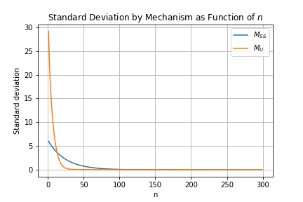
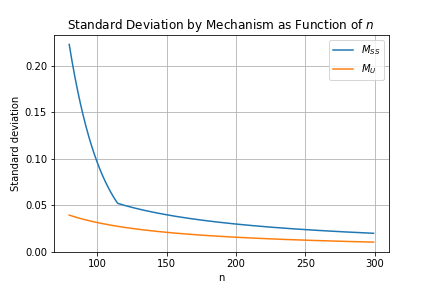
With these settings, we compare the standard deviations (SDs) of the two mechanisms’ mean estimates for a range of sample sizes. Because the mechanisms are unbiased, this is equivalent to their root mean squared error. The sample size estimates of both mechanisms are the same, so we do not report their properties.
Figures 1 and 2 plot the mechanisms’ SDs as functions of , with Figure 2 zooming in on larger values of for clarity. It is immediately clear that the has a larger SD than for , and that this pattern reverses for larger . For , however, both mechanisms have SDs greater than 1, making both unfit for most purposes at these sample sizes, given that the mean has the domain [0,1].
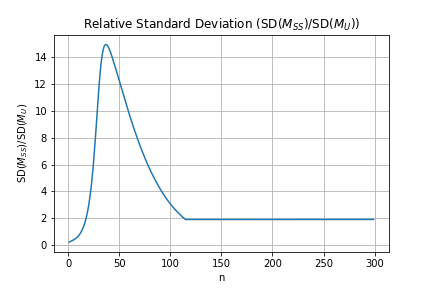
Figure 3 shows the relative SD - that is, the ratio - as a function of . For , the relative SD rises to a peak near 15 before settling down to an apparent constant of about 1.9 for .
Ultimately, appears to be the better mechanism for this setting; for any sample size where either mechanism returns useful results, has a substantially lower SD. The thinner tails of also recommend it as the better choice.
6 Application to Slowly Scaling PRDP
In this section, we use our estimators to develop versions of unbiased privacy mechanisms from [8] that enjoy stronger privacy guarantees. Our estimators allow us to do so while maintaining the mechanisms’ unbiasedness.
-DP guarantees the upper bound on the privacy loss between any pair of neighboring databases. [8] develops mechanisms for a related privacy concept, per-record DP (PRDP) [13]. PRDP generalizes ()-DP by letting the privacy loss bound be a function of the record on which a given pair of neighbors differs. Semantically, this allows different records to have different levels of protection.
Denote a record in the database by and denote ’s attribute by . PRDP was originally motivated by the need to protect data used to compute the sum query . Because the domain of is unbounded, this sum can change by an arbitrarily large amount when a record is added or deleted. That is, the sum’s global sensitivity is infinite. This prevents commonly used privacy mechanisms, such as the Laplace mechanism, from providing a differential privacy guarantee with finite .
The traditional fix for this is to clip attribute to lie in a bounded set before taking the sum. -DP can then be guaranteed by perturbing the sum with noise scaled in proportion to the width of the clipped data’s domain. Unfortunately, when the sum is dominated by a small number of large outliers, the outliers typically need to be clipped to drastically smaller values to preserve a reasonable balance of privacy loss and noise variance. This can induce catastrophic bias, rendering the clipped sums essentially useless. One might expect to see this type of behavior with income data, for example.
PRDP allows us to take a finer look at the privacy-utility tradeoff by recognizing that, even though outliers may suffer extreme privacy loss, the rest of the dataset may still enjoy strong privacy protections. Intuitively, a particular record’s privacy loss is proportional only to the amount by which the addition or deletion of that record can change the query. Queries may be highly sensitive to the presence of outliers while being relatively insensitive to typical records, leading different records to have different levels of privacy loss. The reassurance that the vast majority of the data may enjoy strong privacy guarantees whether or not the data is clipped may allow a data curator to reasonably decide against clipping if the resulting bias outweighs the enhanced privacy protection for a small number of records.
Below, we define PRDP.
Definition 17 (-Per-Record Differential Privacy (-PRDP) [13, 8]).
Let denote the symmetric set difference. The mechanism satisfies per-record differential privacy with the policy function (-PRDP) if, for any record ; any pair of neighboring databases such that ; and any measurable set of possible outcomes , we have
Ensuring strong privacy protection corresponds to ensuring that is, in some sense, small. -DP is recovered by making the constant privacy guarantee for all , and strong privacy protection follows from a small . We cannot always make a guarantee this strong. Take the example where we want to publish a sum query on an unbounded attribute that we are unwilling to clip. In this case, the privacy loss of the mechanisms that we will consider here is growing in . Even though we cannot prevent from growing without bound in , we can use mechanisms for which the growth rate is slow. [8] call such mechanisms “slowly scaling.” A slowly growing narrows the gap in privacy losses between records with large and small values of , letting a data curator more easily provide a desired level of protection for the bulk of the data without compromising too much on the privacy of outliers.
[8] introduces slowly scaling mechanisms, called transformation mechanisms, that work by adding Gaussian noise to a concave transformation of the query (plus offset term) and then feeding the noisy value of to an estimator of . By adding Gaussian noise, these mechanisms satisfy per-record zero-concentrated DP (PRzCDP), which is a weaker privacy guarantee than PRDP. PRzCDP relates to zero-concentrated DP [4, 7] in the same way that PRDP relates to -DP. The use of Gaussian noise also allowed [8] to draw on existing unbiased estimators from [16] to make their mechanism unbiased for a variety of transformation functions .
Using the unbiased estimators from Theorem 10, we strengthen the transformation mechanisms to provide PRDP guarantees by adding Laplace, rather than Gaussian, noise, and we do so without losing the mechanism’s unbiasedness. Algorithm 3 lays out our transformation mechanism.
To obtain the PRDP guarantee of Algorithm 3, we first need to define the per-record sensitivity [8], a record-specific analog of the global sensitivity.
Definition 18 (Per-Record Sensitivity [8]).
The per-record sensitivity of the univariate, real-valued query for record is
Theorem 19 gives our most generic result on the PRDP guarantees of Algorithm 3. Theorems 19 and 20, their proofs, as well as Algorithm 3 are minimally modified from their analogs in [8], which use Gaussian, rather than Laplace noise. This is to facilitate the interested reader’s comparison of our results with theirs.
Theorem 19 (PRDP Guarantee for Transformation Mechanisms).
Assume the query value ; the offset parameter ; the noise scale parameter ; the transformation function is concave and strictly increasing; and the estimator . Denote by the per-record sensitivity of the query , as defined in Definition 18. Algorithm satisfies -PRDP for .
See Appendix D of this paper’s full version (linked to on the title page) for the proof.
Probably the most common query encountered in applications of formal privacy, even as a component of other, larger queries, is the sum query. We now use the above result to derive the policy function for the transformation mechanism applied to a sum query.
Theorem 20 (Privacy of Transformation Mechanisms for Sum Query).
See Appendix D for the proof.
Critically, the policy function from Theorem 20 grows in more slowly when the transformation function grows more slowly. In the case where and for some , the policy function is simply . Choosing larger values of , then, forces the privacy loss to grow more slowly in , reducing the gap in privacy losses between records with large and small values of .
Applying our main results, we can obtain estimators such that the transformation mechanism gives us an unbiased estimate of . In particular, polynomials555In the case of polynomials, [11] derived unbiased estimators which could also be used here. The estimator obtained from our Theorem 10 merely simplifies computation in this setting. are twice differentiable functions which are tempered distributions, so the following holds for :
Corollary 21.
Given any function such that satisfies the conditions in Theorem 10, , , estimator , and for all records , there exists an unbiased estimator for satisfying -PRDP for .
Proof.
7 Polynomial Functions under General Noise Distributions
Additive mechanisms other than the Laplace mechanism, such as the discrete Gaussian or the staircase mechanisms, may be preferable in practice due to achieving higher accuracy while having similar privacy loss [5, 10]. In contrast to the Laplace case, these mechanisms may not admit tractable Fourier transforms, and hence unbiased estimators are generally not available in closed form. One exception is when the query of interest is a polynomial in one or many queries.
Using the following results to obtain an unbiased estimator of a polynomial that approximates a non-polynomial estimand may also allow users to obtain approximately unbiased estimators with great generality.
Theorem 22.
Suppose a mechanism takes as input and outputs for a random variable with at least finite, publicly known moments. If is a polynomial in of degree at most , there exists an unbiased estimator of , which is itself a polynomial of degree at most and is available in closed form.
Proof.
Suppose . Let us find an unbiased estimator of the form . We have
| (18) |
Denote and take expectations to obtain
| (19) | ||||
| (20) |
For this polynomial to be equal to , we need to solve , where and
| (21) |
Clearly, is nondegenerate, and so the desired coefficients exist and are unique.
We now extend this result to polynomials in multiple (univariate) queries, assuming that the noise variables added to each query are independent. The latter assumption, while seemingly restrictive, is typical for additive noise mechanisms in differential privacy.
Theorem 23.
Suppose a mechanism takes as input and outputs for independent random variables with finite, publicly known moments. If is a polynomial in , there exists an unbiased estimator of , which is itself a polynomial available in closed form.
Proof.
Clearly, it suffices to derive unbiased estimators for . Let be the unbiased estimator of as in Theorem 22 and set . Since are independent random variables, we have
| (22) |
8 Conclusions and Future Work
In this work, we have shown how to compute unbiased estimators of twice-differentiable tempered distributions evaluated on privatized statistics with added Laplace noise. In addition, we have proposed a method to extend this result to twice-differentiable functions which are not tempered distributions in a way that achieves approximately optimal expected squared error.
As the Laplace mechanism is simple and commonly used, these results are widely applicable to obtain unbiased statistics for free in postprocessing, which is particularly valuable due to the fact that aggregating unbiased statistics accumulates error more slowly than aggregating biased statistics. We have applied our results to derive a competitive unbiased algorithm for means and to derive unbiased transformation mechanisms for per-record DP mechanisms that enjoy stronger privacy protection than do analogs in previous work. Finally, we have derived an unbiased estimator for polynomials under arbitrary noise distributions with known moments, such as the discrete Gaussian mechanism or the staircase mechanism [5, 10].
We believe this paper opens several avenues for future research. These include the use of the deconvolution method to obtain unbiased estimators for other estimands and noise distributions. We believe a deconvolution method using multivariate Fourier transforms could also be used to obtain unbiased estimators of functions of multivariate queries. Although we did not attempt to optimize the numerical implementation in Section 5 of the integration in Section 4, we believe that an improved implementation could enable the practical use of higher-order polynomial extensions and further reduce error. In Section 7, we developed estimators that are exactly unbiased for polynomials that could approximate other functions of interest. Further work could elaborate on this process, developing concrete procedures for picking the approximating polynomial and deriving bounds on the resulting bias. Finally, future work could attempt to derive noise distributions that are optimal in the sense of minimizing the variances (or other utility metrics) of their unbiased estimators.
References
- [1] John Abowd, Robert Ashmead, Ryan Cumings-Menon, Simson Garfinkel, Micah Heineck, Christine Heiss, Robert Johns, Daniel Kifer, Philip Leclerc, Ashwin Machanavajjhala, Brett Moran, William Sexton, Matthew Spence, and Pavel Zhuravlev. The 2020 Census Disclosure Avoidance System TopDown Algorithm. Harvard Data Science Review, (Special Issue 2), June 24 2022. URL: https://hdsr.mitpress.mit.edu/pub/7evz361i/release/2.
- [2] Daniel Alabi, Audra McMillan, Jayshree Sarathy, Adam Smith, and Salil Vadhan. Differentially private simple linear regression, 2020. arXiv:2007.05157.
- [3] Margaret Beckom, William Sexton, and Anthony Caruso. Researching formal privacy for the Census Bureau’s County Business Patterns program, 2023. URL: https://www.census.gov/data/academy/webinars/2023/differential-privacy-webinar.html.
- [4] Mark Bun and Thomas Steinke. Concentrated differential privacy: Simplifications, extensions, and lower bounds. In Theory of Cryptography Conference, pages 635–658. Springer, 2016. doi:10.1007/978-3-662-53641-4_24.
- [5] Clément L. Canonne, Gautam Kamath, and Thomas Steinke. The discrete Gaussian for differential privacy. In Proceedings of the 34th International Conference on Neural Information Processing Systems, NIPS ’20, Red Hook, NY, USA, 2020. Curran Associates Inc.
- [6] Cynthia Dwork, Frank McSherry, Kobbi Nissim, and Adam Smith. Calibrating noise to sensitivity in private data analysis. Journal of Privacy and Confidentiality, 7(3):17–51, May 2017. doi:10.29012/jpc.v7i3.405.
- [7] Cynthia Dwork and Guy N Rothblum. Concentrated differential privacy. arXiv preprint arXiv:1603.01887, 2016.
- [8] Brian Finley, Anthony M Caruso, Justin C Doty, Ashwin Machanavajjhala, Mikaela R Meyer, David Pujol, William Sexton, and Zachary Terner. Slowly scaling per-record differential privacy. arXiv preprint arXiv:2409.18118, 2024. doi:10.48550/arXiv.2409.18118.
- [9] Jean Baptiste Joseph Fourier. The Analytical Theory of Heat. Cambridge Library Collection - Mathematics. Cambridge University Press, 2009.
- [10] Quan Geng, Peter Kairouz, Sewoong Oh, and Pramod Viswanath. The staircase mechanism in differential privacy. IEEE Journal of Selected Topics in Signal Processing, 9(7):1176–1184, 2015. doi:10.1109/JSTSP.2015.2425831.
- [11] Quentin Hillebrand, Vorapong Suppakitpaisarn, and Tetsuo Shibuya. Unbiased locally private estimator for polynomials of Laplacian variables. In Proceedings of the 29th ACM SIGKDD Conference on Knowledge Discovery and Data Mining, pages 741–751, 2023. doi:10.1145/3580305.3599537.
- [12] Gautam Kamath, Argyris Mouzakis, Matthew Regehr, Vikrant Singhal, Thomas Steinke, and Jonathan Ullman. A bias-variance-privacy trilemma for statistical estimation, 2023. doi:10.48550/arXiv.2301.13334.
- [13] Jeremy Seeman, William Sexton, David Pujol, and Ashwin Machanavajjhala. Privately answering queries on skewed data via per-record differential privacy. Proc. VLDB Endow., 17(11):3138–3150, 2024. doi:10.14778/3681954.3681989.
- [14] Gerrit van Dijk. Distribution Theory. De Gruyter, Berlin, Boston, 2013. doi:doi:10.1515/9783110298512.
- [15] V.G. Voinov and M. Nikulin. Unbiased Estimators and Their Applications Volume 1: Univariate Case. Kluwer Academic Publishers, Dordrecht, 1993.
- [16] Yasutoshi Washio, Haruki Morimoto, and Nobuyuki Ikeda. Unbiased estimation based on sufficient statistics. Bulletin of Mathematical Statistics, 6:69–93, 1956. URL: https://api.semanticscholar.org/CorpusID:55591271.