Mapping the Tradeoffs and Limitations of Algorithmic Fairness

Abstract
Sufficiency and separation are two fundamental criteria in classification fairness. For binary classifiers, these concepts correspond to subgroup calibration and equalized odds, respectively, and are known to be incompatible except in trivial cases. In this work, we explore a relaxation of these criteria based on -divergences between distributions – essentially the same relaxation studied in the literature on approximate multicalibration – analyze their relationships, and derive implications for fair representations and downstream uses (post-processing) of representations. We show that when a protected attribute is determinable from features present in the data, the (relaxed) criteria of sufficiency and separation exhibit a tradeoff, forming a convex Pareto frontier. Moreover, we prove that when a protected attribute is not fully encoded in the data, achieving full sufficiency may be impossible. This finding not only strengthens the case against “fairness through unawareness” but also highlights an important caveat for work on (multi-)calibration.
Keywords and phrases:
Algorithmic fairness, information theory, sufficiency-separation tradeoffCopyright and License:
2012 ACM Subject Classification:
Theory of computation Machine learning theory ; Mathematics of computing Information theory ; Social and professional topics Computing / technology policyAcknowledgements:
We thank Flavio Calmon for an insightful suggestion that inspired the formulation using -information.Funding:
This work was supported in part by a gift to the McCourt School of Public Policy and Georgetown University, Simons Foundation Collaboration 733792, Israel Science Foundation (ISF) grant 2861/20, ERC grant 101125913, and a grant from the Israeli Council for Higher Education. Views and opinions expressed are however those of the authors only and do not necessarily reflect those of the European Union or the European Research Council Executive Agency. Neither the European Union nor the granting authority can be held responsible for them.Editors:
Mark BunSeries and Publisher:
1 Introduction
Machine learning algorithms increasingly influence many aspects of our lives – ranging from seemingly minor decisions, such as which ads appear on a website, to critical financial determinations like loan approvals, and even life-altering outcomes in healthcare and the judicial system. Determining whether and how fairness should be taken into consideration in a specific context; examining whether a particular fairness criterion is suitable, aligns with legal standards, or reflects ethical norms; deciding what trade-offs to strike between the many desiderata one might hold – these quandaries cannot be addressed by math alone. What theoretical computer science can do and has been doing for fairness is to reveal what is possible and what is impossible – for example, what notions can be enforced computationally efficiently and when? What tradeoffs between desiderata are fundamental?
A substantial literature has focused on statistical criteria of group fairness, formalizing various notions of equality across groups or attributes. In this vein, a landmark early result of Chouldechova [3] and of Kleinberg, Mullainathan, and Raghavan [11], revealed that the multiple natural statistical fairness criteria in classification are often inherently incompatible, except in trivial cases.
In this setting, a classification algorithm takes data of an individual as input (for example, her financial history) and outputs some predicted label (for example, whether she is expected to repay a loan). The utility of a classifier or predictor is measured with respect to the true label of the individual (would she actually eventually repay the loan?). Group fairness notions consider some protected attribute (for example, the individual’s ethnicity); each set of people with a particular value of the protected attribute is sometimes referred to as a group or subgroup. The main statistical criteria of fairness in classification are concerned with the statistical relationships that the algorithm induces between the true label, the algorithm’s output, and the protected attribute.
Independence, also known as statistical parity or demographic parity, requires that the predictor’s outcome be independent of the protected attribute. This notion is very restrictive and has been criticized for its seeming unfairness in settings where there exists a correlation between the true label and the protected attribute (see, for example, [5]). It is not a major focus of our study.
Separation, also known as equalized odds [8], requires that the predictor’s outcome be conditionally independent of the protected attribute, given the true label. This means that the distribution of outcomes should be the same across different groups, as long as individuals share the same true label. When the label and the prediction are both binary, this criterion is equivalent to asking for the same true positive rate and true negative rate across the different protected groups. In other words, it guarantees that an imperfect classifier would not err in either direction more on one subgroup than on others.
Sufficiency requires that the protected attribute and the true label be conditionally independent, given the classifier’s prediction. This criterion requires that, among individuals that are given the same prediction, there would be no correlation between the true label and membership in a protected group. In other words, given the outcome of the classifier for an individual, the probability that she has a certain true label should be the same, regardless of her protected attribute. When the true label is binary, sufficiency is equivalent to calibration within subgroups [1]; roughly speaking, a predictor is calibrated if its prediction can be interpreted as the probability of the true label being positive.
1.1 Our contribution
As mentioned above, it is known that separation and sufficiency are often incompatible (although, as we show in Appendix A, they are sometimes compatible in non-trivial scenarios). A common consequence of this impossibility is that researchers and practitioners have been told that they must choose one or the other – separation or sufficiency – but not both. In this work, we propose a relaxation of these statistical criteria of fairness (Section 3.2), study the combinations of these relaxed criteria that are achievable (Lemma 10 and Theorem 12), and show that, in certain scenarios, there exists a continuous, meaningful tradeoff between the relaxed notions, forming a Pareto frontier (Theorem 14). We explore the relationships between the relaxed criteria, see that full sufficiency is not always achievable (Theorem 15), and draw conclusions regarding the post-processing of fair representations – post-processing cannot degrade our notion of approximate separation, but there are conditions on representations under which full sufficiency cannot be recovered by any post-processing (Theorem 17). These results enrich our understanding of the possible fairness tradeoffs that can be achieved, giving policymakers and domain experts a richer design space from which to select.
1.2 Related Work
There has been substantial work on relaxations of the statistical criteria of group fairness. Some approaches weaken the criteria in some non-continuous fashion. This includes, for example, relaxed equalized odds [12] (weakening separation) and equal precision [3] (weakening sufficiency), both of which are motivated by the incompatibility results, in an attempt to find weaker fairness notions that are compatible with each other. A major motivation for equal opportunity [8] (a relaxation of separation) in contrast, is compatibility with higher prediction accuracy than the stronger notion of equalized odds.
More continuous relaxations have primarily appeared in the contexts of learning and optimization. They typically involve the definition of some approximation or error term that quantifies how much a predictor violates the desired criterion, and then use this term either as an objective or as a penalty or regularization term in the learning objective of the predictor; such work has not focused on the compatibilities that such relaxations enable. Examples include Zafar et al. [16] and Woodworth et al. [15], who propose moment-based approximations in order to solve the intractability of the optimization problem, as well as Zemel et al. [17] and Bechavod and Ligett [2], who define a regularization term in order to achieve independence and separation, respectively. Of particular relevance to our work are Kashima et al. [10], who use mutual information as a regularization term for learning classifiers that satisfy independence, and Gopalan et al. [6], who define the objective of multicalibration [9] in terms of average conditional covariance (as discussed in Section 3.3).
Perhaps most closely related to our work is the analysis of Hamman and Dutta [7], who adopt an information-theoretic perspective with very similar definitions to ours. However, their analysis – based on partial information decomposition – focuses only on scenarios where at least one of the fairness criteria is fully met.
2 Preliminaries
Statistical notions of fairness focus on the aggregate properties of a population rather than of any particular individual. The literature on fair classification typically considers the relationships between three variables when defining statistical criteria for fairness: the true label (or target variable) , the protected attribute (or subgroup) , and the predictor’s outcome . In principle, all relationships between these variables are possible (see Figure 1(a)), and various fairness notions can be seen as restrictions on the relationships between these variables.
Interestingly, the data upon which the predictor makes the prediction (or is learned), , is usually not explicitly modeled. In the multicalibration literature [9], however, the data does play a central role, as all the variables and are defined as (possibly stochastic) functions of (see Figure 1(b)). If this is the case, not all relationships between and are possible. In particular, under this model, , meaning that all the information about the true label that is encoded in the protected attribute is also encoded in the data .
In this work we consider a model that generalizes these two approaches: we explicitly include the data in our model, but we do not assume that and are functions only of , thus allowing for more complex relationships between them (see Figure 1(c)). This model can capture any joint distribution without any further assumptions, with determined exclusively by the conditional distribution .
Moreover, we prefer to view as a representation of the data – either an explicit representation that can be passed to some end-user, or an inner state of a model – and not necessarily as the final prediction or classification, which can be made upon this representation. This view allows for greater flexibility and raises interesting points with respect to post-processing.
2.1 Statistical Criteria for Fair Classification
As mentioned above, the main statistical criteria for fair classification are defined in terms of statistical independence of the three variables , and :
Definition 1 (Statistical criteria for fair classification).
Let , and be jointly distributed random variables, representing the true label, a protected attribute and the predictor’s outcome, accordingly. Then,
- Independence
-
requires the predictor’s outcome to be independent of the protected attribute: . Specifically, for all and , .
- Separation
-
requires the predictor’s outcome to be conditionally independent of the protected attribute, given the value of the true label: . Specifically, for all , and , .
- Sufficiency
-
requires the true label and the protected attribute to be conditionally independent of each other, given the predictor’s outcome: . Specifically, for all , and , .
In this work we focus on separation and sufficiency, as independence is usually too restrictive.
2.2 Notation
Throughout this paper, we use capital letters for random variables, their respective lower case letters for their realizations, and script for the alphabet, as in . The notation is short for . For simplicity, we assume that all variables are finite; if, for example, naturally takes values in , we consider a suitable quantization.
3 Relaxing the Statistical Criteria of Fairness
A notable result in algorithmic fairness due to Chouldechova [3] and Kleinberg, Mullainathan, and Raghavan [11] states that for binary classification, separation and sufficiency cannot simultaneously hold except in trivial cases – either when and are independent (meaning that different groups share the same base rate for the true label, eliminating any inherent fairness concerns), or when the predictor perfectly predicts . More generally, they show that if and are not independent and the joint distribution of , , and has full support (meaning that every combination of these variables has nonzero probability), then sufficiency and separation are fundamentally incompatible. (In Appendix A we show that there are non-trivial (though limited) settings where separation and sufficiency are compatible.)
Considering this incompatibility, we may look for suitable relaxations of the notions of separation and sufficiency, and analyze the relationships between the relaxed criteria. Since both criteria are defined in terms of statistical independence, one natural relaxation is to quantify the deviation from independence using (conditional) mutual information. We adopt a slightly more general approach, using -information – a measure of statistical association based on -divergences, which generalizes the well-established concept of mutual information.
3.1 -Divergences and -Information
The next section provides the essential background on -divergences and -information, including definitions and key properties.
Definition 2 (-Divergence).
Let be a convex function with , and let and be two probability distributions over the same space. The -divergence of from is defined as
where the second equality holds for discrete distributions with the conventions that , and for . For a complete definition and analysis, see [13, Chapter 7].
Some important examples of -divergences are the Kullback-Leibler (KL) divergence, taking to obtain (note that the expectation is over ); the total variation (TV), with yielding ; and the -divergence, with . The Rényi divergences, although not -divergences, are closely related and share many of their properties.
The following is a useful property of -divergences.
Proposition 3.
[13, Theorem 7.5] For any -divergence , . If is strictly convex at 1, then iff .
In all the examples above, is indeed strictly convex at 1.
Inspired by the definition of mutual information, a similar measure of association between random variables can be defined using -divergences:
Definition 4 (-Information).
Let and be random variables with joint distribution and respective marginals and . The -information between and is defined as
that is, the -divergence between their joint distribution and the product distribution of their marginals.
Let be another jointly distributed random variable. Then, the conditional -information between and given is defined as
For KL divergence, -information is exactly Shannon’s mutual information. For TV, is closely related to the covariance (see Proposition 8).
The following property of -information is an immediate consequence of Proposition 3 and the definition of statistical independence.
Proposition 5 (-Information and independence).
If is strictly convex at 1, then
(If is not strictly convex at 1, then independence still implies zero information, but not vice versa.)
We highlight another important property of -information – the data processing inequality (DPI):
Proposition 6 (Data processing inequality).
[13, Theorem 7.16] Let random variables form a Markov chain in that order, meaning that . Then
3.2 Relaxing the Fairness Criteria
In light of Proposition 5, the statistical criteria for fair classification, which are defined in terms of conditional independence, can be relaxed using the notion of -information.
Definition 7 (Deviations from fairness criteria).
Let , and be jointly distributed random variables, and let be an -information. We define
- Deviation from Independence
-
as ,
- Deviation from Separation
-
as , and
- Deviation from Sufficiency
-
as .
Each of these quantities measures to what extent the joint distribution of , and diverges from the statistical independence that defines the respective criterion, where a value of zero means that the criterion is fully satisfied. When the specific -information is of relevance, we may write for clarity. We sometimes refer to the original statistical criteria as, e.g., “full separation” and “full sufficiency” to distinguish them from these relaxed notions.
An additional relevant quantity that is closely related to the deviations above is , which expresses the amount of “information” that the predictor conveys about the true label . This can be seen as a measure of the predictor’s overall performance, similar to its accuracy. It can be shown that maximizing (using KL divergence) is equivalent to minimizing the expected cross-entropy loss, , which is a common practice in the optimization of classifiers.111Note that , where the first term, , is the entropy of and does not depend on , and the second term is the negative of the expected cross-entropy loss (see, e.g., [4]).
3.3 Interpreting the Relaxed Criteria
The definition of the relaxed criteria in terms of -information (Definition 7) may not seem intuitive at first. However, applying Bayes’ rule and some algebra transforms these expressions into a form that more closely resembles the original definitions of the fairness criteria. Consider, for example, the deviation from separation:
This expression represents the expected divergence between the conditional distribution of given both and , and its conditional distribution given only . In other words, it quantifies how much, on average (over the values of and ), the predictor’s outcome distribution within the subgroups differs from the average in the population, among individuals that share the same true label.
Similarly, for the deviation from sufficiency we have
| (1) |
that is, the average difference between the the true label distribution within the subgroups and its average in the population, among individuals that share the same predicted value.
One potential drawback of using -information to define relaxed fairness criteria is its average-case nature. In particular, smaller subgroups – especially those where certain labels or prediction values are rare – contribute less to the deviation. One could argue that this is an unfair approach to fairness. In any case, some of our results treat scenarios where one or more of the deviations is zero, in which case taking the average or the maximum yields the same result.
To address this drawback, some works instead use a maximum-based approach to defining relaxed group fairness criteria (see, for example, [15]). However, placing excessive weight on rare examples can introduce statistical biases and negatively impact the learning process of fair predictors and representations. This very concern has led the multicalibration literature [9, 6] to adopt a relaxed objective that is essentially equivalent to TV-information, as we demonstrate next.
Following the definition in [6], a predictor is said to be -approximate subgroup calibrated with respect to if it satisfies .
Proposition 8.
Let , and be jointly distributed random variables, and assume that and take values in . Then, is -approximate subgroup calibrated with respect to iff .
The proof, provided in Appendix B, relies on the fact that in the binary case, . More generally, for and that take on numeric values, denote the ranges and . Then we have .
Finally, Pinsker’s inequality [13, Theorem 7.10] states that (when KL divergence is taken with the natural logarithm), meaning that using KL divergence for the deviation dominates the use of total variation. In particular, this gives .
4 Main Results
Given that the criteria of full separation and full sufficiency cannot always be satisfied simultaneously, our primary goal is to address the following question:
For any given setting (defined by , , and ), what are the best combinations of deviations from sufficiency and separation that are achievable?
This question leads us to formalize the following definition:
Definition 9 (The separation-sufficiency function).
Let , and be jointly distributed finite random variables. We define the separation-sufficiency function as
for all , such that the set above is not empty.
Since , we know from Proposition 3 that the separation-sufficiency tradeoff function is nonnegative. In what follows, we prove that is attained as a minimum and it is continuous and convex. Moreover, we show that in certain settings it is monotonically nonincreasing, and in others it is bounded away from zero – two properties with important implications.
4.1 The Achievable Region and the Separation-Sufficiency Curve
Consider any joint distribution . Any choice of a predictor – that is, a choice of a conditional distribution – corresponds to a point in the nonnegative octant representing the triplet . We refer to the set of all such possible points as the achievable region. We first show that the achievable region (as illustrated in Figure 2) is convex and compact.
Lemma 10 (Convexity of the achievable region).
Let , and be jointly distributed finite random variables. The associated achievable region, that is, the set
is convex and compact.
Proof.
Denote by the set of all probability distributions over the alphabet of . For all , define the following functions:
Define the function as , and let be the convex hull of the image of in . Finally, define , that is, the “slice” of that corresponds to the marginal of in the first coordinate.
Since is finite, is finite dimensional and compact, and since is continuous, the set is both convex and compact. Consequently, so is , as an intersection with a hyperplane.
We will now show that , that is, the achievable region of . Indeed, if , then by its definition and the definition of a convex hull, there exist , and with , such that
| (2) |
Define a predictor according to the conditional distribution , for all and . This distribution is well-defined, since by (2), . In addition, we have , and therefore by Bayes’ rule, . Moreover, clearly form a Markov chain, because is defined in terms of alone. Now, substituting and in (2), it can be shown that , and (see Appendix C for a detailed derivation).
Conversely, if there exists a finite random variable , such that form a Markov chain, then following the approach in Appendix C, we get that , and . In other words, is a convex combination of the points , with the weights given by , and thus by its definition, . Consequently, .
It is worth noting that the definition of the achievable region can be extended to include , while preserving its convexity and compactness. The proof is a straightforward extension of the arguments above.
The connection between the achievable region and the separation-sufficiency function is emphasized in the following corollary:
Corollary 11.
The separation-sufficiency function is a continuous convex curve, and it is attained as a minimum.
Proof.
Let , that is, the projection of the achievable region onto the first two coordinates, which correspond to and . By Lemma 10, is convex and compact, implying the same for the projection . The claim now follows from the observation that the curve is the lower boundary of .
The next result further characterizes the function and establishes its domain.
Theorem 12.
Let , and be jointly distributed finite random variables and denote by
the set of all achievable values of deviation from separation, corresponding to all possible predictors. Then
For the proof, we use the following bound:
Proposition 13.
Let , , and be jointly distributed random variables, such that form a Markov chain. Then .
Proof.
This follows from the data processing inequality for the Markov chain , conditioned on each value of , so that .
Proof of Theorem 12.
Since , Proposition 3 implies that all satisfy . Let be a constant predictor, that is, . Then meets the Markov condition and . Therefore, the bound is tight.
On the other hand, by Proposition 13, all satisfy . Let be the identity predictor. Then satisfies the Markov condition and . Therefore, the bound is also tight.
Finally, since is the projection of the achievable set onto the first coordinate, and since is convex and compact by Lemma 10, must be a closed interval in . Consequently, following the bounds above, .
The proof shows that the predictors and attain the left and right bounds of , respectively. Since we have and , and the achievable region is convex, we conclude that the line segment between the points and is contained in , the projection of onto the first two coordinates (see Figure 2(a)). In particular, this implies the following bounds on the right endpoint of :
| (3) |
4.2 The Separation-Sufficiency Tradeoff
If both and are determined by (possibly stochastic) functions of , then all the information about the true label that is encoded in the protected attribute is also encoded in the data . This assumption is common in the multicalibration literature, where denotes either a subset of [9], or more generally a real valued function of [6]. It is equivalent to saying that form a Markov chain, that , or – most importantly for our analysis – that . In this case, we say that the data itself satisfies sufficiency.
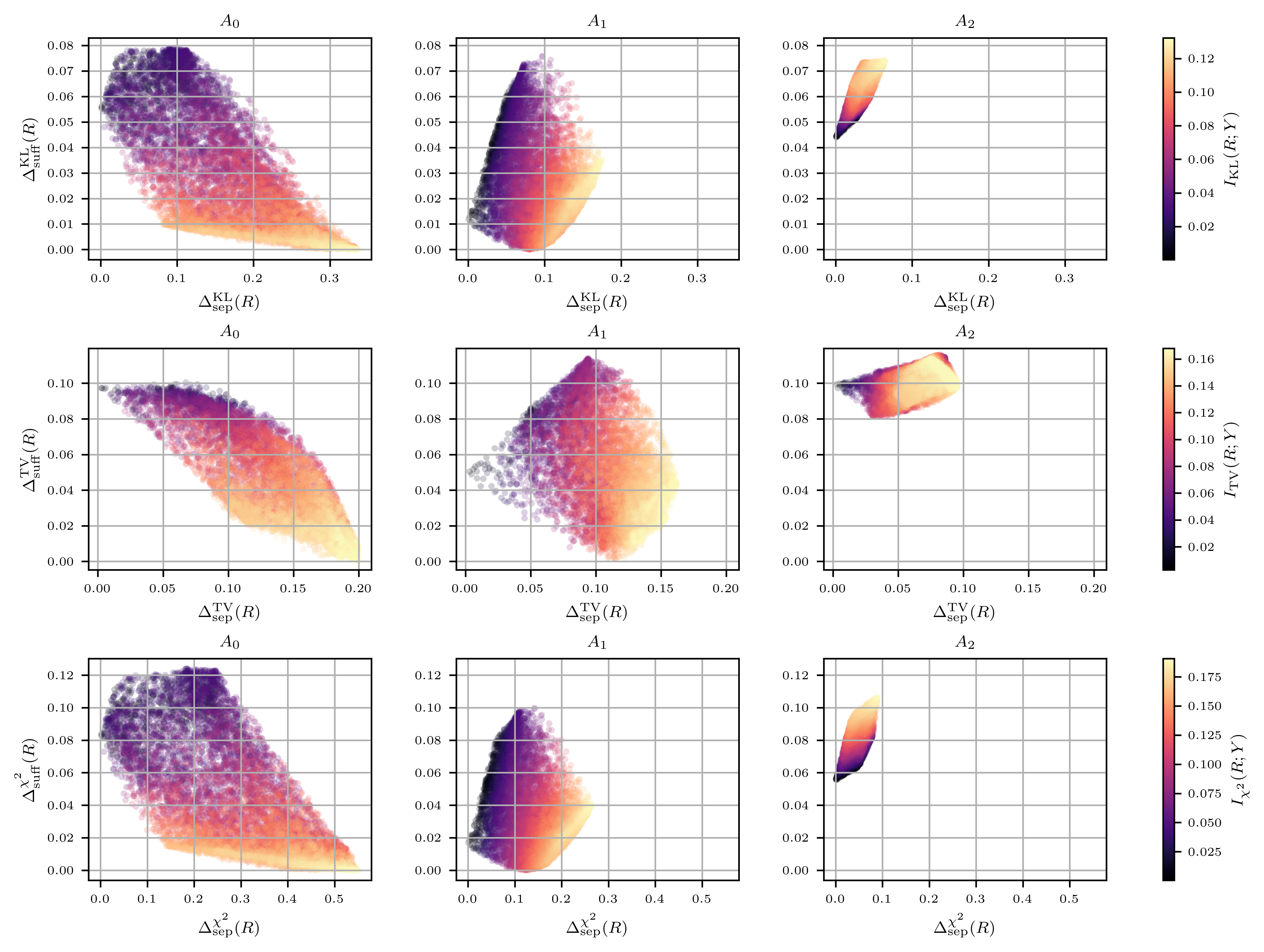
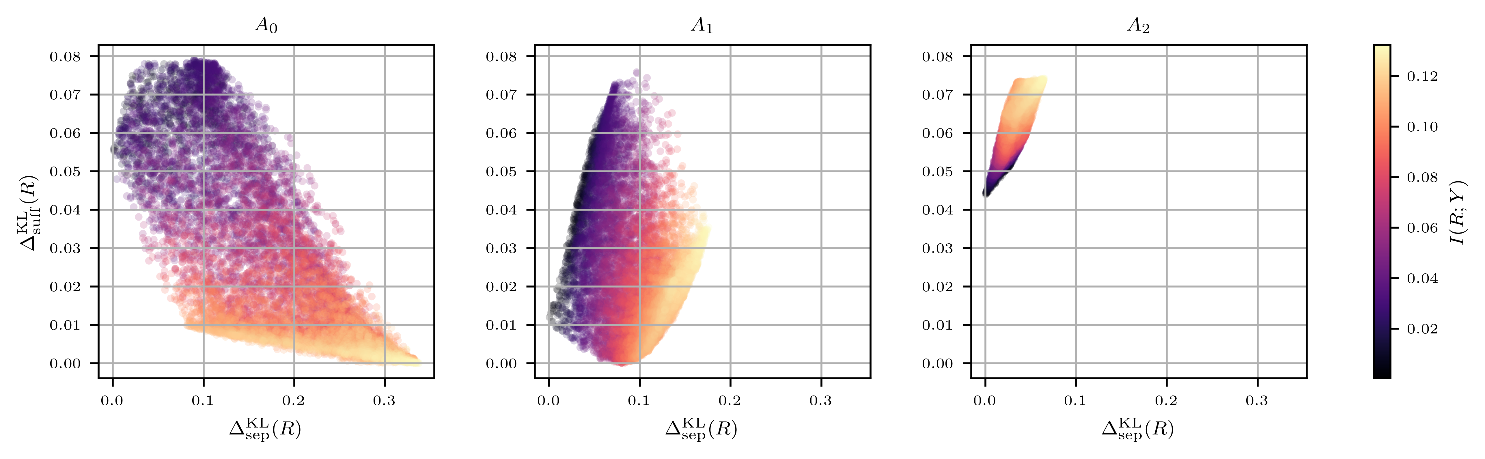
In this specific setting, as we prove in the following theorem, the separation-sufficiency curve is monotonically nonincreasing, and thus represents a Pareto frontier of fairness, reflecting the fundamental tradeoff between separation and sufficiency (see Figure 2(b) for a schematic, and the left panel of Figure 3 for a simulation).
Theorem 14 (The separation-sufficiency tradeoff).
Let , and be jointly distributed finite random variables, such that . Then the separation-sufficiency curve is convex, nonincreasing in , and attains the value zero. In particular, there exist predictors that satisfy sufficiency.
Proof.
From Corollary 11 and Theorem 12, we know that ) is convex for all . In addition, the assumption that , meaning that , together with (3), implies that . Since is attained as a minimum, it follows that there exist predictors that satisfy sufficiency (in particular, the identity predictor ).
Let . From convexity, we have
Since , and , we conclude that , that is, . This means that is monotonically nonincreasing in .
This result shows that, rather than needing to abandon either separation or sufficiency due to their incompatibility, a parametric approach reveals a continuous tradeoff between the measures of deviation from those criteria, exposing a range of intermediate combinations that can be achieved.
For example, suppose that a predictor was trained to achieve no worse than a certain subgroup calibration error. This objective corresponds to a level of deviation from sufficiency, and may be compatible with a quite good level of separation. The convexity of the curve suggests that a small relaxation of the subgroup calibration objective can result in a relatively large improvement in the separation measure.
4.3 Full Sufficiency Is Unachievable When the Data Is Not Rich Enough
The previous result relies heavily on the assumption that the data itself satisfies sufficiency. When this is not the case, that is, when , it means that the data is not expressive enough to convey all the information about the relationship between the protected attribute and the true label . This can occur if the protected attribute is not an inherent part of the data, yet it bears information about the true label. In particular, this can happen when the protected attribute is deliberately stripped from the data, as in the practice of “fairness through unawareness.”
In this case, there is no guarantee that the separation-sufficiency curve is monotonic (see an example of such a situation in the middle panel of Figure 3), nor that it attains the value zero (see Figure 3, right panel). In other words, there is no guarantee that there exist predictors that satisfy perfect sufficiency. In fact, we show that in certain scenarios such predictors do not exist.
In the following analysis, we rely exclusively on Shannon’s mutual information, as it allows us to apply its chain rule (see, for example, [4]), which does not necessarily have a counterpart in other forms of -information.
Theorem 15.
Let , and be jointly distributed finite random variables. Then for all in its domain, the separation-sufficiency function using mutual information satisfies .
Proof.
Let be a predictor defined by the conditional distribution , meaning that form a Markov chain. In particular, form a Markov chain too, and thus by the data processing inequality we have
| (4) |
Now, using the chain rule of mutual information in two different ways, we get
Therefore, , and from (4) it follows that
| (5) |
Finally, let . Then by Corollary 11, is attained by some predictor , such that and . Substituting these equalities in (5) yields .
Corollary 16.
If then there exists no predictor that satisfies sufficiency.
Proof.
By Theorem 15 we have . Since is the lower boundary of the achievable region, this means that no predictor attains .
(Note that, although the statement of the corollary is in terms of Shannon’s mutual information, the result that holds for all -information with strictly convex at 1, since in that case implies sufficiency.)
It is worth noting that when form a Markov chain, the data processing inequality guarantees that , and thus this corollary does not contradict Theorem 14.
This result has important implications when considering downstream uses of representations (post-processing), as we explore in the next section.
4.4 Post-Processing
Our analysis of the achievable region, along with the tradeoffs and limitations of separation and sufficiency, has some straightforward implications for the downstream use of fair representations. Specifically, note that when is regarded as a representation, upon which a further prediction will be made, then takes the place of in our model (Figure 1(c)). This is formalized in the next result.
Theorem 17 (Post-processing).
Let , and be jointly distributed finite random variables. If and are two finite random variables, such that form a Markov chain in that order, we say that the predictor is a post-processing of , or a downstream predictor based on . We have the following results:
-
1.
If is a post-processing of , then , meaning that the deviation from separation cannot increase with post-processing.
-
2.
If satisfies sufficiency, then the separation-sufficiency curve restricted to downstream predictors is convex, nonincreasing, and attains the value zero.
-
3.
If satisfies , then for any post-processing we have , meaning that no downstream predictor can satisfy sufficiency.
Proof.
Note that if is a post-processing of then, in particular, form a Markov chain. Therefore,
Note that, as a consequence of the first result above, if satisfies full separation then any downstream predictor will necessarily satisfy full separation too – essentially collapsing the space of possible tradeoffs with sufficiency. This is especially restrictive when taking into account that separation is fundamentally at odds with , the amount of relevant information that the predictor conveys about the true label (see Appendix D).
Regarding statement 3, it should be noted that by the data processing inequality, , meaning that the quantity can only decrease with post-processing, running the risk that repeated or aggressive post-processing of a representation can result in a state where full sufficiency is no longer achievable.
5 Discussion
We hope that this work contributes to elucidating the possible tradeoffs between various desiderata that are achievable in the design of classification algorithms, providing a richer space of options to domain experts and decision-makers.
Although we have primarily focused on separation-sufficiency tradeoffs, the tradeoff is, in fact, triple – between separation, sufficiency, and performance, as measured by . In particular, there may exist several predictors that attain a specific point on the separation-sufficiency curve, with different levels of overall performance. In Appendix D we make a first step in this direction, and provide an analysis of the tension between separation and the predictor’s performance. This is a promising direction for future research.
Furthermore, our focus in this work has been information theoretic – exploring the possible tradeoffs that predictors can achieve; developing algorithms to efficiently compute such predictors is an interesting open question.
References
- [1] Solon Barocas, Moritz Hardt, and Arvind Narayanan. Fairness and Machine Learning: Limitations and Opportunities. MIT Press, 2023.
- [2] Yahav Bechavod and Katrina Ligett. Penalizing unfairness in binary classification. arXiv preprint arXiv:1707.00044, 2017.
- [3] Alex Chouldechova. Fair prediction with disparate impact: A study of bias in recidivism prediction instruments. Big Data, 5(2):153–163, October 2016. doi:10.1089/BIG.2016.0047.
- [4] Thomas M. Cover and Joy A. Thomas. Elements of Information Theory. Wiley-Interscience, 2nd ed. edition, 2006.
- [5] Cynthia Dwork, Moritz Hardt, Toniann Pitassi, Omer Reingold, and Richard Zemel. Fairness through awareness. In 3rd Innovations in Theoretical Computer Science Conference (ITCS), pages 214–226, 2012. doi:10.1145/2090236.2090255.
- [6] Parikshit Gopalan, Adam Tauman Kalai, Omer Reingold, Vatsal Sharan, and Udi Wieder. Omnipredictors. In 13th Innovations in Theoretical Computer Science Conference (ITCS), volume 215, pages 79:1–79:21, 2022. doi:10.4230/LIPICS.ITCS.2022.79.
- [7] Faisal Hamman and Sanghamitra Dutta. A unified view of group fairness tradeoffs using partial information decomposition. In 2024 IEEE International Symposium on Information Theory (ISIT), pages 214–219, 2024. doi:10.1109/ISIT57864.2024.10619698.
- [8] Moritz Hardt, Eric Price, and Nathan Srebro. Equality of opportunity in supervised learning. Advances in Neural Information Processing Systems, 29, 2016.
- [9] Ursula Hébert-Johnson, Michael Kim, Omer Reingold, and Guy Rothblum. Multicalibration: Calibration for the (computationally-identifiable) masses. In International Conference on Machine Learning, pages 1939–1948. PMLR, 2018.
- [10] Toshihiro Kamishima, Shotaro Akaho, and Jun Sakuma. Fairness-aware learning through regularization approach. In 2011 IEEE 11th International Conference on Data Mining Workshops, pages 643–650, 2011. doi:10.1109/ICDMW.2011.83.
- [11] Jon Kleinberg, Sendhil Mullainathan, and Manish Raghavan. Inherent Trade-Offs in the Fair Determination of Risk Scores. In 8th Innovations in Theoretical Computer Science Conference (ITCS), pages 43:1–43:23, 2017. doi:10.4230/LIPICS.ITCS.2017.43.
- [12] Geoff Pleiss, Manish Raghavan, Felix Wu, Jon Kleinberg, and Kilian Q Weinberger. On fairness and calibration. Advances in Neural Information Processing Systems, 30, 2017.
- [13] Yury Polyanskiy and Yihong Wu. Information Theory: From Coding to Learning. Cambridge University Press, 2025.
- [14] Hans S. Witsenhausen and Aaron D. Wyner. A conditional entropy bound for a pair of discrete random variables. IEEE Transactions on Information Theory, 21(5):493–501, 1975.
- [15] Blake Woodworth, Suriya Gunasekar, Mesrob I. Ohannessian, and Nathan Srebro. Learning non-discriminatory predictors. In Conference on Learning Theory, pages 1920–1953. PMLR, 2017. URL: http://proceedings.mlr.press/v65/woodworth17a.html.
- [16] Muhammad Bilal Zafar, Isabel Valera, Manuel Gomez Rodriguez, and Krishna P Gummadi. Fairness beyond disparate treatment & disparate impact: Learning classification without disparate mistreatment. In Proceedings of the 26th International Conference on World Wide Web, pages 1171–1180, 2017. doi:10.1145/3038912.3052660.
- [17] Rich Zemel, Yu Wu, Kevin Swersky, Toniann Pitassi, and Cynthia Dwork. Learning fair representations. In International Conference on Machine Learning, pages 325–333. PMLR, 2013.
Appendix A Achieving Separation and Sufficiency Together
If and are not independent, then separation and sufficiency cannot simultaneously hold if the joint distribution of , and has full support [3, 11]. In the binary case, this means that separation and sufficiency can be achieved together only if perfectly predicts . However, in the general case, this does not always result in trivial or degenerate conditions.
Indeed, assume that satisfies both and . The first condition means that form a Markov chain in that order. From the data processing inequality for mutual information we have . The second condition means that form a Markov chain, and thus . Together, we get that , meaning that and convey the same information about . In other words, this implies that is a sufficient statistic of for (see, for example, [4]).
The following is an example of such a case, where full separation and full sufficiency are not incompatible:
Example 18.
Let for some . For , let , where and . Define , that is, the value of the binary word , and . Then
From this definition of , we see that the sequence forms a Markov chain. In other words, is conditionally independent of given , meaning that it satisfies full separation.
A simple calculation shows that also satisfies full sufficiency. For example,
Consequently, even though is not independent of , we have an example of a predictor that satisfies both separation and sufficiency, and yet does not allow for a perfect estimation of (for example, if , then can be either 1, 2 or 4). The predictor is indeed a sufficient statistic of for —it can be seen in the matrix above that for all , the probability does not distinguish between values of that correspond to binary words with the same number of ones, which is exactly the value of .
Appendix B Deviation from Sufficiency and Multicalibration
Following Definition 5.3 in [6], a predictor is said to be -approximate subgroup calibrated with respect to if it satisfies .
Proposition 19.
Let , and be jointly distributed random variables, and assume that and take values in . Then is -approximate subgroup calibrated with respect to iff .
Proof.
We show that when and are binary, . Indeed,
so we have .
In a similar way, it can be also shown that
Therefore,
Now, using total variation to measure the deviation from sufficiency, we get from (1) that
Appendix C Details for the Proof of Lemma 10
From (2) we have . Substituting for and for we get
| (6) | ||||
| (7) | ||||
| (8) | ||||
| (9) |
where (6) is simply the definition of ; (7) follows from the Markov assumption, , so and ; and (8) and (9) are due to Bayes’ rule, as and .
Similar steps show that and .
Appendix D Separation Is at Odds with the Predictor’s Overall Performance
The criterion of separation has sometimes been criticized (see, for example, [1, Chapter 3]) because imposing equal error rates across subgroups often leads to suboptimal performance for some of them. In this appendix we formalize this argument—that separation may conflict with the overall performance quality of the predictor.
Indeed, in addition to the tradeoff between separation and sufficiency, the convexity of the achievable region (Lemma 10) also implies a similar tradeoff between separation and . As noted earlier, this quantity can be interpreted as a measure of the predictor’s overall performance. The analysis below builds on the same reasoning as that of the separation-sufficiency tradeoff.
Definition 20 (The separation-performance function).
Let , and be jointly distributed finite random variables. We define the separation-performance function as
for all .
Note that the domain of follows from Theorem 12.
Theorem 21 (The separation-performance tradeoff).
The separation-performance function is continuous, concave, monotonically nondecreasing in , and attained as a maximum.
Proof.
Recall the definition of the achievable region,
and denote by the projection of onto the first and third coordinates, corresponding to and . By Lemma 10, the achievable region is convex and compact, implying the same for its projection . Since is the upper boundary of , it follows that it is a continuous concave curve. In addition, the compactness of implies that is attained as a maximum.
Let . Since is attained as a maximum, there exists a predictor forming a Markov chain , such that and . By the data processing inequality we have , and thus
| (10) |
Now, denote by the identity predictor. Then and . Therefore, by its definition, , and together with (10) we get that .
Finally, let . From concavity, we have
Since by (10), , and , we conclude that ; that is, . This means that is monotonically nondecreasing in .
This result is of particular concern if serves as a representation, upon which further predictions will be made. The reason is that imposing a low deviation from separation already at an upstream stage may decrease the information that bears on the true label ; by the data processing inequality, this in turn will constrain all downstream predictors.
Appendix E Simulation of the Achievable Region
We provide the details and full results of the simulation that we ran in order to visualize the achievable region in concrete examples, corresponding to different settings of , and .
E.1 Method
First, we fix a joint distribution . We then consider three different cases of , corresponding to three distinct scenarios:
For each of these scenarios we draw at random 10,000 conditional distributions in the following manner: denote by the size of the alphabet of , then by Carathéodory-Fenchel-Eggleston theorem (see, e.g., [14, Lemma 2.2]), every point in the achievable region can be attained by a predictor taking as most values. Hence, for each sampling of a distribution , it suffices to draw distributions from , the probability simplex over points. We do that using an -dimensional Dirichlet distribution.
For each choice of , we calculate , and , using different -divergences. Finally, we plot the points corresponding to the 10,000 sampled predictors in the plane, colored according to their respective value of .
E.2 Details
We considered taking 4 values, and binary and . Specifically, we fixed and , as well as the following conditional distributions for :
-
1.
with , so that .
-
2.
and .
-
3.
and .
See Table 1 for the resulting values of , , and .
| KL divergence | Total variation | -divergence | |||||||
|---|---|---|---|---|---|---|---|---|---|
| 0.000 | 0.036 | 0.074 | 0.000 | 0.045 | 0.098 | 0.000 | 0.041 | 0.107 | |
| 0.338 | 0.177 | 0.066 | 0.200 | 0.162 | 0.096 | 0.553 | 0.267 | 0.090 | |
| 0.393 | 0.152 | 0.035 | 0.224 | 0.148 | 0.070 | 0.583 | 0.251 | 0.049 | |
| 0.055 | 0.011 | 0.044 | 0.098 | 0.048 | 0.099 | 0.081 | 0.016 | 0.055 | |
For each , as explained above, we sampled 4 distribution vectors (corresponding to the values of ) from a 5-dimensional symmetric Dirichlet distribution with parameter . The resulting plots are shown in Figure 4.