The Correlated Gaussian Sparse Histogram Mechanism

Lebeda, Christian Janos; Retschmeier, Lukas

doi:10.4230/LIPIcs.FORC.2025.23

The Correlated Gaussian Sparse Histogram Mechanism

Christian Janos Lebeda

Inria, University of Montpellier, France Lukas Retschmeier

BARC, University of Copenhagen, Denmark

Abstract

We consider the problem of releasing a sparse histogram under $(\varepsilon,\delta)$ -differential privacy. The stability histogram independently adds noise from a Laplace or Gaussian distribution to the non-zero entries and removes those noisy counts below a threshold. Thereby, the introduction of new non-zero values between neighboring histograms is only revealed with probability at most $\delta$ , and typically, the value of the threshold dominates the error of the mechanism. We consider the variant of the stability histogram with Gaussian noise.
Recent works ([Joseph and Yu, COLT ’24] and [Lebeda, SOSA ’25]) reduced the error for private histograms using correlated Gaussian noise. However, these techniques can not be directly applied in the very sparse setting. Instead, we adopt Lebeda’s technique and show that adding correlated noise to the non-zero counts only allows us to reduce the magnitude of noise when we have a sparsity bound. This, in turn, allows us to use a lower threshold by up to a factor of $1/2$ compared to the non-correlated noise mechanism. We then extend our mechanism to a setting without a known bound on sparsity. Additionally, we show that correlated noise can give a similar improvement for the more practical discrete Gaussian mechanism.

Keywords and phrases:

differential privacy, correlated noise, sparse gaussian histograms

Copyright and License:

2012 ACM Subject Classification:

Security and privacy

\rightarrow

Privacy-preserving protocols

Related Version:

Full Version: https://arxiv.org/abs/2412.10357 [17]

Funding:

Retschmeier carried out this work at Basic Algorithms Research Copenhagen (BARC), which was supported by the VILLUM Foundation grant 54451. Providentia, a Data Science Distinguished Investigator grant from the Novo Nordisk Fonden, supported Retschmeier. The work of Lebeda is supported by grant ANR-20-CE23-0015 (Project PRIDE).

DOI:

10.4230/LIPIcs.FORC.2025.23

Event:

6th Symposium on Foundations of Responsible Computing (FORC 2025)

Editors:

Mark Bun

Series and Publisher:

Leibniz International Proceedings in Informatics, Schloss Dagstuhl – Leibniz-Zentrum für Informatik

1 Introduction

Releasing approximate counts is a common task in differential private data analysis. For example, the task of releasing a search engine log, where one wants to differentially private release the number of users who have searched each possible search term.

The full domain of search terms is too large to work with directly, but the vector of all search counts is extremely sparse as most phrases are never searched. The standard approach to exploit sparsity while ensuring differential privacy is the stability histogram [3, 15, 5, 1, 12, 13, 25]. The idea is to preserve sparsity by filtering out zero counts and then adding noise from a suitable probability distribution to the remaining ones. Unfortunately, some filtered-out counts could be non-zero in a neighboring dataset, and thus, revealing any of them would violate privacy. To limit this privacy violation, the stability histogram introduces a threshold $\tau$ and releases only those noisy counts that exceed $1+\tau$ . This way, we might still reveal the true dataset among a pair of neighboring datasets if one of these counters exceeds the threshold, but with an appropriate choice of $\tau$ , this is extremely unlikely to happen.

In our setting, one single user may contribute to many counts; hence, using the Gaussian Sparse Histogram Mechanism (GSHM) [12, 24] might be preferable. The GSHM is similar to the stability histogram, but it replaces noise from the Laplace distribution with Gaussian noise. To analyze the $(\varepsilon,\delta)$ guarantees of the GSHM, one has to find an upper bound for $\delta$ , which is influenced by the standard Gaussian mechanism and the small probability of infinite privacy loss that can happen when the noise exceeds $\tau$ . We denote these two quantities as $\delta_{\text{\footnotesize{gauss}}}$ and $\delta_{\text{\footnotesize{inf}}}$ . Recently, [24] gave exact privacy guarantees of the GSHM, which improves over the analysis by [12] where $\delta_{\text{\footnotesize{gauss}}}$ and $\delta_{\text{\footnotesize{inf}}}$ were simply summed. Their main contribution is a more intricate case distinction of a single user’s impact on the values of $\delta_{\text{\footnotesize{gauss}}}$ and $\delta_{\text{\footnotesize{inf}}}$ . This allows them to use a lower threshold with the same privacy parameters. Their improvement lies in the constants, but it can be significant in practical applications because the tighter analysis essentially gives better utility at no privacy cost.

Our goal is to reduce the error further. Because the previous analysis is exact, we must exploit some additional structure of the problem. Consider a $d$ -dimensional histogram $H(\mathbf{X})=\sum_{i=1}^{n}X_{i}$ for $\mathbf{X}=(X_{1},\dots,X_{n})$ for users with data $X_{i}\in\{0,1\}^{d}$ . Notice that adding a single user to $\mathbf{X}$ can only increase counts in $H(\mathbf{X})$ , whereas removing one can only decrease counts. Lebeda [16] recently showed how to exploit this monotonicity by adding a small amount of correlated noise. This reduces the total magnitude of noise almost by a factor of $2$ compared to the standard Gaussian Mechanism. So, it is natural to ask if we can adapt this technique to the setting when the histogram is sparse. This motivates our main research question:

Question: When can we take advantage of monotonicity and use correlated noise to improve the Gaussian Sparse Histogram Mechanism?

1.1 Our Contribution

We answer this question by introducing the Correlated Stability Histogram (CSH). Building on the work by [16], we extend their framework to the setting of releasing a histogram under a sparsity constraint, that is $\|H(\mathbf{X})\|_{0}\leq k$ for some known $k$ . This is a natural setting that occurs e.g. for Misra-Gries sketches, where $k$ is the size of the sketch [21, 18]. Furthermore, enforcing this sparsity constraint is necessary to achieve the structure required to benefit from correlated noise.

Correlated GSHM.

We introduce the Correlated Stability Histogram (CSH), a variant of the GSHM using correlated noise. Our algorithm achieves a better utility-privacy trade-off than GSHM for $k$ -sparse histograms. Similar to the result of Lebeda [16], we show that correlated noise can reduce the error by almost a factor of $2$ at no additional privacy cost. In particular, our main result lies in the following (informally stated) theorem:

Theorem 1 (The Correlated Stability Histogram Mechanism (Informal)).

Let $H(\mathbf{X})=\sum_{i}^{n}X_{i}$ denote a histogram with bounded sparsity, where $\mathbf{X}=(X_{1},\dots,X_{n})$ and $X_{i}\in\{0,1\}^{d}$ . If the GSHM privately releases $H(\mathbf{X})$ under $(\varepsilon,\delta)$ -DP with noise magnitude $\sigma$ and removes noisy counters below a threshold $\tau$ , then the Correlated Stability Histogram Mechanism (CSH) releases $H(\mathbf{X})$ also under $(\varepsilon,\delta)$ -DP with noise of magnitude ${\sigma}/{2}+o(1)$ and removes noisy counters below a threshold ${\tau}/{2}+o(1)$ .

As a baseline, we first analyze our mechanism using the add-the-deltas [12] approach and show that even this approach outperforms the exact analysis in [25] in many settings. We then turn our attention to a tighter analysis, which uses an intricate case distinction to upper bound the parameter $\delta$ . Furthermore, we complement our approach with the following results:

Generalization & Extensions.

We extend our mechanism to multiple other settings, including extensions considered in [24]. First, we generalize our approach to allow an additional threshold that filters out infrequent data in a pre-processing step. Second, we discuss how other aggregate database queries can be included in our mechanism. Last, we generalize to top- $k$ counting queries when we have no bound for $\|H(\mathbf{X})\|_{0}$ .

Discrete Gaussian Noise.

Our mechanism achieves the same improvement over GSHM when noise is sampled from the discrete Gaussian rather than the continuous distribution. We present a simple modification to make our mechanism compatible with discrete noise. This has practical relevance even for the dense setting considered by Lebeda [16].

Organization.

The rest of the paper is organized as follows. Section 2 introduces the problem formally and reviews the required background. Section 3 introduces the Correlated Stability Histogram, our main algorithmic contribution for the sparse case. Furthermore, in Section 4 we generalize our approach to the non-sparse setting. The extensions of our technique to match the setting of Wilkins et al. [24] are discussed in Section 6. In Section 7, we show how to adapt our mechanism for discrete Gaussian noise. Finally, we conclude the paper in Section 8 and discuss open problems for future work.

Additionally, numerical evaluations in Section 5 confirm our claim that we improve the error over previous techniques.

2 Preliminaries and Background

Given a dataset $\mathbf{X}\in\mathcal{U}^{*}$ , where $\mathcal{U}^{*}\coloneqq\bigcup_{m=0}^{\infty}\mathcal{U}^{m}$ is the set of datasets with any size, we want to perform an aggregate query $\mathcal{A}$ under differential privacy. We focus on settings where each user has a set of elements, and we want to estimate the count of all elements over the dataset. Therefore, we consider a dataset $\mathbf{X}=(X_{1},\dots,X_{n})$ of $n$ data points where each $X_{i}\in\{0,1\}^{d}$ . Our goal is to output a private estimate of the histogram $H(\mathbf{X})\in\mathbb{N}^{d}$ , where $H(\mathbf{X})=\sum_{i=1}^{n}X_{i}$ ¹¹1Note that in the differential privacy literature the term histogram is often used for the special case where users each have a single element. We use it for consistency with related work (e.g. [24]). The setting we consider is closely related to the problem of releasing one-way marginals.. For any vector $\mathbf{H}\in\mathbb{R}^{d}$ , we define the support as $U(\mathbf{H})=\{i\in[d]:H_{i}\neq 0\}$ and denote the $\ell_{0}$ norm as $\|\mathbf{H}\|_{0}\coloneqq|U(\mathbf{H})|$ , being the number of non-zeroes in $\mathbf{H}$ . In this work, we focus on settings where the dimension $d$ is very large or infinite.

Proposed by [10], differential privacy (DP) is a property of a randomized mechanism. The intuition behind differential privacy is that privacy is preserved by ensuring that the output distribution does not depend much on any individual’s data. In this paper, we consider $(\varepsilon,\delta)$ -differential privacy (sometimes referred to as approximate differential privacy) together with the add-remove variant of neighboring datasets as defined below. Note that by this definition $|\mathbf{X}|=n$ and $|\mathbf{X}^{\prime}|=n\pm 1$ :

Definition 2 (Neighboring datasets).

A pair of datasets are neighboring if there exists an $i$ such that either $\mathbf{X}=(X^{\prime}_{1},\dots,X^{\prime}_{i-1},X^{\prime}_{i+1},\dots,X^{% \prime}_{n+1})$ or $\mathbf{X}^{\prime}=(X_{1},\dots,X_{i-1},X_{i+1},\dots,X_{n})$ holds. We denote the neighboring relationship as ${\mathbf{X}\sim\mathbf{X}^{\prime}}$ .

Definition 3 ([11] $(\varepsilon,\delta)$ -differential privacy).

Given $\varepsilon$ and $\delta$ , a randomized mechanism $\mathcal{M}:\mathcal{U}^{*}\rightarrow\mathcal{Y}$ satisfies $(\varepsilon,\delta)$ -DP, if for every pair of neighboring datasets $\mathbf{X}\sim\mathbf{X}^{\prime}$ and every measurable set of outputs $Y\in\mathcal{Y}$ it holds that

\Pr[\mathcal{M}(\mathbf{X})\in Y]\leq e^{\varepsilon}\Pr[\mathcal{M}(\mathbf{X% }^{\prime})\in Y]+\delta\,.

We shortly denote the case where $\delta=0$ as $\varepsilon$ -DP. Differential privacy is immune to post-processing. Let $\mathcal{M}:\mathcal{U}^{*}\rightarrow R$ be a randomized algorithm that is $(\varepsilon,\delta)$ -DP. Let $f:R\rightarrow R^{\prime}$ be an arbitrary randomized mapping. Then $f\circ\mathcal{M}:\mathcal{U}^{*}\rightarrow R^{\prime}$ is $(\varepsilon,\delta)$ -DP.

An important concept in differential privacy is the sensitivity of a query, which restricts the difference between the output for any pair of neighboring datasets. We consider both the $\ell_{2}$ sensitivity and, more generally, the sensitivity space of the queries in this paper.

Definition 4 (Sensitivity space and $\ell_{2}$ sensitivity).

The sensitivity space of a deterministic function $f:\mathcal{U}^{*}\rightarrow\mathbb{R}^{d}$ is the set $\Delta f=\{f(\mathbf{X})-f(\mathbf{X}^{\prime})\in\mathbb{R}^{d}\mid\mathbf{X}% \sim\mathbf{X}^{\prime}\}$ and denote $\|\mathbf{x}\|_{2}=\sqrt{\sum_{i=1}^{d}x_{i}^{2}}$ as the $\ell_{2}$ norm of any $\mathbf{x}\in\mathbb{R}^{d}$ . Then the $\ell_{2}$ sensitivity of $f$ is defined as

\Delta_{2}f=\max_{\mathbf{X}\sim\mathbf{X}^{\prime}}\|f(\mathbf{X})-f(\mathbf{% X}^{\prime})\|_{2}=\max_{\mathbf{x}\in\Delta f}\|\mathbf{x}\|_{2}\,.

The standard Gaussian mechanism adds continuous noise from a Gaussian distribution to $f(\mathbf{X})$ with magnitude scaled according to Lemma 5.

Lemma 5 ([4, Theorem 8] The Analytical Gaussian Mechanism).

Let $f:\mathcal{U}^{*}\rightarrow\mathbb{R}^{d}$ denote a function with $\ell_{2}$ sensitivity at most $\Delta_{2}$ . Then the mechanism that outputs $f(X)+(Z_{1},\cdots,Z_{d})$ , where each $Z_{i}\sim\mathcal{N}(0,\sigma^{2})$ are independent and identically distributed, satisfies $(\varepsilon,\delta)$ -differential privacy if the following inequality holds

\delta\geq\Phi\left(\frac{\Delta_{2}}{2\sigma}-\frac{\varepsilon\sigma}{\Delta% _{2}}\right)-e^{\varepsilon}\Phi\left(-\frac{\Delta_{2}}{2\sigma}-\frac{% \varepsilon\sigma}{\Delta_{2}}\right)

where $\Phi(X)$ denotes the cdf of the Gaussian distribution.

2.1 The Gaussian Sparse Histogram Mechanism

Refer to caption — Figure 1: Examples of different kinds of neighboring datasets for the Gaussian Sparse Histogram Mechanism where a single user can contribute to at most four counters, thus $\|X_{i}\|_{0}\leq 4$ . These counters are depicted in green. a) For the example on the left, the mechanism behaves exactly as running the Gaussian mechanism on a restricted domain. b) In the case in the middle, we only have to bound the probability that one of the green elements together with the additive noise term exceeds the threshold $1+\tau$ . c) The case on the right is the most difficult case for the privacy analysis because the overall $\delta$ value depends on both kinds of changes.

We consider the problem of releasing the histogram $H(\mathbf{X})$ of a dataset ${\mathbf{X}=(X_{1},\cdots,X_{n})}$ where each $X_{i}\in\{0,1\}^{d}$ under differential privacy. The standard techniques for releasing a private histogram are the well-known Laplace mechanism [10] and Gaussian mechanism [9, 4], which achieve $\varepsilon$ - and $(\varepsilon,\delta)$ -DP, respectively. Although this works well for dense data, it is unsuited for very sparse data where $\|H(\mathbf{X})\|_{0}\ll d$ because adding noise to all entries increases both the maximum error as well as the space and time requirements. Furthermore, the mechanisms are undefined for infinite domains ( $d=\infty$ ).

In the classic sparse histogram setting where $\|X_{i}\|_{0}=1$ , the preferred technique under $(\varepsilon,\delta)$ -DP is the stability histogram which combines Laplace noise with a thresholding technique (see [3, 15, 5, 1, 12, 13, 25]).

In this paper, we consider the Gaussian Sparse Histogram Mechanism (see [12, 24]), which replaces Laplace noise in the stability histogram with Gaussian noise. This is often preferred when users can contribute multiple items as the magnitude of noise is scaled by the $\ell_{2}$ sensitivity instead of the $\ell_{1}$ sensitivity. The GSHM adds Gaussian noise to each non-zero counter of $H(\mathbf{X})$ and removes all counters below a threshold $1+\tau$ . Find the pseudocode in Algorithm 1. We discuss the impact of the parameter $\tau$ below.

Algorithm 1 The Gaussian Sparse Histogram Mechanism (GSHM).

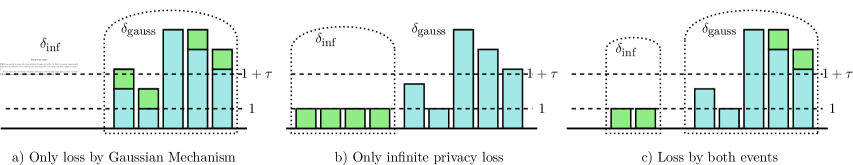
To get $(\varepsilon,\delta)$ differential privacy guarantees, we observe that there are two sources of privacy loss that have to be accounted for by the value of $\delta$ : $\delta_{\text{\footnotesize{gauss}}}$ from the Gaussian noise itself and the probability of infinite privacy loss $\delta_{\text{\footnotesize{inf}}}$ , when a zero count is deterministically ignored in one dataset, but possibly released in a neighboring one. These events have infinite privacy loss because they can only occur for one of the datasets. Therefore, $\delta_{\text{\footnotesize{inf}}}$ bounds the possibility of outputting a counter that is not present in the neighboring dataset. Figure 1 gives some intuition about the role of $\delta_{\text{\footnotesize{gauss}}}$ and $\delta_{\text{\footnotesize{inf}}}$ . Throughout this section, we assume that $\|X_{i}\|_{0}\leq k$ for some known integer $k\ll d$ .

2.2 The add-the-deltas Approach

The following approach appeared in a technical report in the Google differential privacy library [12]. Similar techniques have been used elsewhere in the literature (e.g. [25]). We refer to this technique as add-the-deltas. We have to account for the privacy loss due to the magnitude of the Gaussian noise. Therefore, the value of $\delta_{\text{\footnotesize{gauss}}}$ is typically found by considering the worst-case effect of a user that only changes non-zero counters in both histograms. The value of $\delta_{\text{\footnotesize{gauss}}}$ follows from applying Lemma 5 (compare also Figure 1a) ).

The event of infinite privacy loss is captured by $\delta_{\text{\footnotesize{inf}}}$ . This is bounded by considering the worst-case scenario of changing $k$ zero-counters to $1$ and the fact that infinite privacy loss occurs exactly when any of these $k$ counters exceed the threshold in the non-zero dataset (compare Figure 1b) ).

The observation for the add-the-deltas approach is that $\delta_{\text{\footnotesize{gauss}}}+\delta_{\text{\footnotesize{inf}}}$ is a valid upper bound on the overall $\delta$ value, and hence the condition of Lemma 6 is sufficient to achieve differential privacy.

Lemma 6 ([12] add-the-deltas).

If pairs of neighboring histograms differs in at most $k$ counters then the Gaussian Sparse Histogram Mechanism with parameters $\sigma$ and $\tau$ satisfies $(\varepsilon,\delta_{\text{\footnotesize{gauss}}}+\delta_{\text{\footnotesize{% inf}}})$ -differential privacy where

\displaystyle\delta_{\text{\footnotesize{gauss}}}

\displaystyle=\Phi\left(\frac{\sqrt{k}}{2\sigma}-\frac{\varepsilon\sigma}{% \sqrt{k}}\right)-e^{\varepsilon}\Phi\left(-\frac{\sqrt{k}}{2\sigma}-\frac{% \varepsilon\sigma}{\sqrt{k}}\right),\quad\text{and}\quad\delta_{\text{% \footnotesize{inf}}}=1-\Phi\left(\frac{\tau}{\sigma}\right)^{k}\,.

2.3 Exact Analysis by Taking the Max over the Sensitivity Space

While the add-the-deltas approach is sufficient to bound $\delta$ it does not give the tightest possible parameters. Wilkins et al. [24] were able to derive an exact value for $\delta$ . Compared to the add-the-deltas approach above, the key insight is that the two worst-case scenarios cannot occur simultaneously for any pair of neighboring histograms. This means that each counter either contributes to $\delta_{\text{\footnotesize{gauss}}}$ or $\delta_{\text{\footnotesize{inf}}}$ , but never to both. In the extreme cases, either all $k$ counters flip from zero to one, from one to zero, or none of them do between neighboring datasets. Thus, we only need to consider a single source of privacy loss. In the other (mixed) cases, we have to consider both sources of privacy loss, but the change is smaller than for the worst-case pair of datasets. A small example is depicted in Figure 1. Wilkins et al. [24] used this fact to reduce the threshold required to satisfy the given privacy parameters using a tighter analysis. We now restate their main result: the exact privacy analysis of the GSHM.

Lemma 7 ([24] Exact Privacy Analysis of the GSHM).

If pairs of neighboring histograms differs in at most $k$ counters then the Gaussian Sparse Histogram Mechanism with parameters $\sigma$ and $\tau$ satisfies $(\varepsilon,\delta)$ -differential privacy where $\gamma(j)=(k-j)\log\Phi\left(\frac{\tau}{\sigma}\right)$ and

	$\displaystyle\delta\geq\max\bigg{[}1-\Phi\left(\frac{\tau}{\sigma}\right)^{k},$
	$\displaystyle\max_{j\in[k]}1-\Phi\left(\frac{\tau}{\sigma}\right)^{k-j}+\Phi% \left(\frac{\tau}{\sigma}\right)^{k-j}\left[\Phi\left(\frac{\sqrt{j}}{2\sigma}% -\frac{(\varepsilon-\gamma(j))\sigma}{\sqrt{j}}\right)-e^{\varepsilon-\gamma(j% )}\Phi\left(-\frac{\sqrt{j}}{2\sigma}-\frac{\left(\varepsilon-\gamma(j)\right)% \sigma}{\sqrt{j}}\right)\right],$
	$\displaystyle\max_{j\in[k]}\Phi\left(\frac{\sqrt{j}}{2\sigma}-\frac{\left(% \varepsilon+\gamma(j)\right)\sigma}{\sqrt{j}}\right)-e^{\varepsilon+\gamma(j)}% \Phi\left(-\frac{\sqrt{j}}{2\sigma}-\frac{(\varepsilon+\gamma(j))\sigma}{\sqrt% {j}}\right)\bigg{]}\,.$

Note that we use a slightly different convention from [24]. We use a threshold of $1+\tau$ rather than $\tau$ . Furthermore, they also consider a more general mechanism that allows for optional aggregation queries and an additional threshold parameter. Although our work can easily be adapted to this setting as well, these extensions are not the focus of our main work to simplify presentation. A discussion of the extensions can be found in Section 6.

2.4 The Correlated Gaussian Mechanism

Our work builds on a recent result by Lebeda [16] about using correlated noise to improve the utility of the Gaussian mechanism under the add-remove neighboring relationship. They show that when answering $d$ counting queries, adding a small amount of correlated noise to all queries can reduce the magnitude of Gaussian noise by almost half. We restate their main result for $(\varepsilon,\delta)$ -differential privacy with a short proof as they use another privacy definition.

Lemma 8 ([16] The Correlated Gaussian Mechanism).

Let $H(\mathbf{X})\coloneqq\sum_{i=1}^{n}X_{i}$ where $X_{i}\in\{0,1\}^{d}$ . Then the mechanism that outputs $H(\mathbf{X})+Z_{cor}{\textbf{1}^{d}}+(Z_{1},\cdots,Z_{d})$ satisfies $(\varepsilon,\delta)$ -DP. Here ${\textbf{1}^{d}}$ is the $d$ -dimensional vector of all ones, $Z_{cor}\sim\mathcal{N}(0,\sigma^{2}/\gamma)$ , and each $Z_{i}\sim\mathcal{N}(0,\sigma^{2})$ where

\displaystyle\delta\geq\Phi\left(\frac{\sqrt{d+\gamma}}{4\sigma}-\frac{2% \varepsilon\sigma}{\sqrt{d+\gamma}}\right)-e^{\varepsilon}\Phi\left(-\frac{% \sqrt{d+\gamma}}{4\sigma}-\frac{2\varepsilon\sigma}{\sqrt{d+\gamma}}\right)\,.

Proof.

This follows from combining the inequality for the standard Gaussian mechanism (see Lemma 5) with [16, Lemma 3.5]. Furthermore, if we set $\gamma=\sqrt{d}$ as in [16, Theorem 3.1] we minimize the total magnitude of noise. Notice that the value of $\sigma$ scales with $\sqrt{d}$ for the standard Gaussian mechanism and it scales with $\frac{1}{2}\sqrt{d+\gamma}=\frac{1}{2}\sqrt{d+\sqrt{d}}$ here. We add two noise samples to each query, and the total error for each data point scales with $\frac{1}{2}\sqrt{d+\gamma+d/\gamma+1}=(\sqrt{d}+1)/2$ . $\hfill\blacktriangleleft$

Concurrently with the result discussed above, [14] considered the setting where user contributions are sparse such that $\|X_{i}\|_{0}\leq k$ for some $k\leq d/2$ . They give an algorithm that adds the optimal amount of correlated Gaussian noise for any $d$ and $k\leq d/2$ . It is natural to ask whether this algorithm can improve error for our setting since they focus on a sparse setting. However, their improvement factor over the standard Gaussian mechanism depends on the sparsity. Naively applying their technique for the setting of the GSHM where $k\ll d$ yields no practical improvements. We instead focus on adapting the technique from [16]. We discuss a more restrictive setting where the technique of [14] applies in Section 8.

3 Algorithmic Framework

We are now ready to introduce our main contribution, a variant of the Gaussian Sparse Histogram Mechanism using correlated noise. We first introduce our definition of $k$ -sparse monotonic histograms. Throughout this section, we assume that all histograms are both $k$ -sparse and monotonic. Intuitively, we define monotonicity on a histogram in a way that captures the setting where the counts are either all increasing or all decreasing. Observe that due to the monotonicity constraint, we have that the supports $U$ and $U^{\prime}$ for two neighboring histograms satisfy either $U\subseteq U^{\prime}$ or $U^{\prime}\subseteq U$ . We use this property in the privacy proofs later. The histograms are also monotonic in [24], but they do not require $k$ -sparsity. We provide a mechanism for a setting where the histograms are not $k$ -sparse in Section 4. There we enforce the sparsity constraint using a simple pre-processing step. Both sparsity and monotonicity are required in order to achieve the structure between neighboring histograms required to benefit from correlated noise.

Definition 9 ( $k$ -sparse monotonic histogram).

We assume that the input histogram is $k$ -sparse. That is, for any dataset $\mathbf{X}$ we have $\|H(\mathbf{X})\|_{0}\leq k$ . Furthermore, the sensitivity space of $H$ is $\{0,1\}^{d}\cup\{0,-1\}^{d}$ . That is, the difference between counters of neighboring histograms are either non-decreasing or non-increasing.

One example of $k$ -sparse monotonic histograms is Misra-Gries sketches. Merging Misra-Gries sketches is common in practical applications. The sensitivity space of merged Misra-Gries sketches of size $k$ exactly matches Definition 9 (See [18]). Our algorithm is more general than Misra-Gries sketches and satisfies differential privacy as long as the structure between neighboring histograms holds for all pairs of neighboring datasets.

Notice that Definition 9 implies that neighboring histograms differ in at most $k$ counters. As such, we can release the histogram using the standard Gaussian Sparse Histogram Mechanism. Wilkins et al. [24] already uses the fact that counters are either non-decreasing or non-increasing in their analysis. We intend to further take advantage of the monotonicity by adding a small amount of correlated noise to all non-zero counters. This allows us to reduce the total magnitude of noise similar to [16]. The reduced magnitude of noise in turn allows us to reduce the threshold required for privacy. The pseudocode for our mechanism is in Algorithm 2.

Algorithm 2 Correlated Stability Histogram (CSH).

We first give privacy guarantees for Algorithm 2 in a (relatively) simple closed form similar to the add-the-deltas approach. Later, we give tighter bounds using a more complicated analysis similar to Lemma 7. Unfortunately, the proofs from previous work in either case rely on the fact that all noisy counters are independent. That is clearly not the case for our mechanism because the value of $Z_{cor}$ is added to all entries. Instead, we use different techniques to give similar results, starting with the add-the-deltas approach. The following lemma gives a general bound for the event that one of $j$ correlated noisy terms exceeds a threshold $\tau$ . We use this in the proof for both approaches later.

Lemma 10 (Upper bound for Correlated Noise).

Let $Z_{\scriptstyle\text{corr}}\sim\mathcal{N}(0,\sigma^{2}/\sqrt{k})$ be a single sample for a real $k>0$ together with $j$ additional samples $Z_{1},\dots,Z_{j}\sim\mathcal{N}(0,\sigma^{2})$ . Then for any $\tau>0$ , we have $\Pr[\exists i\in[j]:Z_{\scriptstyle\text{corr}}+Z_{i}>\tau]\leq 1-\Phi\left({% \tau}/\left({\sigma\left(k^{-1/4}+1\right)}\right)\right)^{j+1}$ .

Proof.

The proof is in Section B.2. $\hfill\blacktriangleleft$

3.1 The add-the-deltas Analysis

The following Theorem 11 proves privacy guarantees of our mechanism using a similar technique than the one proposed by the Google Anonymization Team [12] and Wilson et al. [25] which is known as add-the-deltas. The total value for $\delta$ is split between $\delta_{\text{\footnotesize{gauss}}}$ and $\delta_{\text{\footnotesize{inf}}}$ which accounts for the two types of privacy loss that are relevant to the mechanism. Like with the GSHM, these values are found by considering worst-case pairs of neighboring histograms for each case. However, a pair of neighboring histograms cannot be worst-case for both values as seen in Figure 1 which motivates the tighter analysis later in the section.

Theorem 11 (add-the-deltas technique).

Algorithm 2 satisfies $(\varepsilon,\delta_{\text{\footnotesize{gauss}}}+\delta_{\text{\footnotesize{% inf}}})$ -differential privacy for $k$ -sparse monotonic histograms where

	$\displaystyle\delta_{\text{\footnotesize{gauss}}}$	$\displaystyle=\Phi\left(\frac{\sqrt{k+\sqrt{k}}}{4\sigma}-\frac{2\varepsilon% \sigma}{\sqrt{k+\sqrt{k}}}\right)-e^{\varepsilon}\Phi\left(-\frac{\sqrt{k+% \sqrt{k}}}{4\sigma}-\frac{2\varepsilon\sigma}{\sqrt{k+\sqrt{k}}}\right)$
	$\displaystyle\delta_{\text{\footnotesize{inf}}}$	$\displaystyle=1-\Phi\left(\frac{\tau}{\sigma\left(1+k^{-1/4}\right)}\right)^{k% +1}\,.$

Proof.

By Definition 3, the lemma holds if for any pair of neighboring $k$ -sparse monotonic histograms $H(\mathbf{X})$ and $H(\mathbf{X}^{\prime})$ and all sets of outputs $Y$ we have

\Pr[CSH(H(\mathbf{X}))\in Y]\leq e^{\varepsilon}\Pr[CSH(H(\mathbf{X}^{\prime})% )\in Y]+\delta_{\text{\footnotesize{gauss}}}+\delta_{\text{\footnotesize{inf}}% }\,.

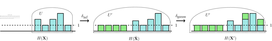
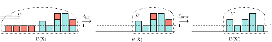
We prove that the inequality above holds by introducing a third histogram. This new histogram is constructed such that it is between $H(\mathbf{X})$ and $H(\mathbf{X}^{\prime})$ . We first state the desired properties of this histogram and then show that such a histogram must exist for all neighboring histograms. Assume for now that there exists a histogram $H(\hat{\mathbf{X}})\in\mathbb{N}^{d}$ where the following two inequalities hold for any set of outputs $Y$ :

	$\displaystyle\Pr[CSH(H(\hat{\mathbf{X}}))\in Y]$	$\displaystyle\leq e^{\varepsilon}\Pr[CSH(H(\mathbf{X}^{\prime}))\in Y]+\delta_% {\text{\footnotesize{gauss}}}\,,$		(1)
	$\displaystyle\Pr[CSH(H(\mathbf{X}))\in Y]$	$\displaystyle\leq\Pr[CSH(H(\hat{\mathbf{X}}))\in Y]+\delta_{\text{% \footnotesize{inf}}}\,.$		(2)

Then the inequality we need for the lemma follows immediately since

	$\displaystyle\Pr[CSH(H(\mathbf{X}))\in Y]$	$\displaystyle\leq\Pr[CSH(H(\hat{\mathbf{X}}))\in Y]+\delta_{\text{% \footnotesize{inf}}}$
		$\displaystyle\leq e^{\varepsilon}\Pr[CSH(H(\mathbf{X}^{\prime}))\in Y]+\delta_% {\text{\footnotesize{gauss}}}+\delta_{\text{\footnotesize{inf}}}\,.$

Next, we show how to construct $H(\hat{\mathbf{X}})$ from $H(\mathbf{X})$ and $H(\mathbf{X}^{\prime})$ , and finally we show that each of two inequalities holds using this construction. Let $U=\{i\in[d]:H(\mathbf{X})_{i}\neq 0\}$ denote the support of $H(\mathbf{X})$ and define similarly $U^{\prime}$ and $\hat{U}$ . We construct $H(\hat{\mathbf{X}})$ such that it has the same support as $H(\mathbf{X}^{\prime})$ , that is $U^{\prime}=\hat{U}$ . For all $i\in(U\cap U^{\prime})$ we set $H(\hat{\mathbf{X}})_{i}=H({\mathbf{X}})_{i}$ and for all $i\notin(U\cap U^{\prime})$ we set $H(\hat{\mathbf{X}})_{i}=H(\mathbf{X}^{\prime})_{i}$ . In other words, we construct $H(\hat{\mathbf{X}})$ such that (1) $H(\mathbf{X}^{\prime})$ and $H(\hat{\mathbf{X}})$ only differ in entries that are in both $U$ and $U^{\prime}$ (2) $H({\mathbf{X}})$ and $H(\hat{\mathbf{X}})$ only differ in entries that are in only one of $U$ and $U^{\prime}$ . This allows us to analyze each case separately to derive our values for $\delta_{\text{\footnotesize{gauss}}}$ and $\delta_{\text{\footnotesize{inf}}}$ . An example of this construction is shown in Figure 2.

We start with the case of $\delta_{\text{\footnotesize{gauss}}}$ using $H(\mathbf{X}^{\prime})$ and $H(\hat{\mathbf{X}})$ . Let ${CSH^{\prime}}$ denote a new mechanism equivalent to Algorithm 2 except that the condition on line 5 is removed. Notice that with $H(\mathbf{X}^{\prime})$ or $H(\hat{\mathbf{X}})$ as inputs ${CSH^{\prime}}$ is equivalent to the Correlated Gaussian Mechanism restricted to $U^{\prime}$ . Since $|U^{\prime}|\leq k$ we have by Lemma 8 that

\Pr[{CSH}^{\prime}(H(\hat{\mathbf{X}}))\in Y]\leq e^{\varepsilon}\Pr[{CSH}^{% \prime}(H(\mathbf{X}^{\prime}))\in Y]+\delta_{\text{\footnotesize{gauss}}}\,.

Notice that if we post-process the output of ${CSH}^{\prime}$ by removing entries below $1+\tau$ , then the output distribution is equivalent to $C S H$ . Equation 1 therefore holds because post-proccessing does not affect differential privacy guarantees (see Definition 3).

The histograms $H(\mathbf{X})$ and $H(\hat{\mathbf{X}})$ only differ in entries that all have a count of $1$ in one of the histograms while they all have a count of $0$ in the other. $\delta_{\text{\footnotesize{inf}}}$ accounts for the event where any such counter exceeds the threshold because the distributions are identical for the shared support. The probability of this event is increasing in the number of different elements between $H(\mathbf{X})$ and $H(\hat{\mathbf{X}})$ and therefore, the worst case happens for neighboring datasets such that $H(\mathbf{X})=\mathbf{1}^{k}$ and $H(\hat{\mathbf{X}})=\mathbf{0}^{k}$ . Note that this bound also hold when zero counters in $H(\mathbf{X})$ are non-zero in $H(\hat{\mathbf{X}})$ . We focus on one direction because the proof is almost identical for the symmetric case. We bound the probability of outputting any entries from $H(\mathbf{X})$ , that is $\tilde{H}_{i}:=1+Z_{\scriptstyle\text{corr}}+Z_{i}>1+\tau$ for at least one $i\in(U\setminus U^{\prime})$ . The bound for $\delta_{\text{\footnotesize{inf}}}$ follows from setting $j=k$ in Lemma 10. $\hfill\blacktriangleleft$ In Section B.1, we show how to directly compute the required threshold based on the result in Theorem 11.

3.2 Tighter Analysis

Next, we carry out a more careful analysis that considers all elements from the sensitivity space similar to [24]. As discussed above, we cannot directly translate the analysis by Wilkins et al. because they rely on independence between each entry. Due to space constraints, we refer the full proof to the full version of the paper [17], and we only give a short intuition behind the theorem here.

Theorem 12 (Tighter Analysis).

First define $\gamma(j)=\min\left(\sqrt{j},\dfrac{1}{2}\sqrt{j+\sqrt{k}}\right)$ , $\psi(m)=\Phi\left(\frac{\tau}{(1+k^{-1/4})\sigma}\right)^{m+1}$ , and $\hat{\varepsilon}(j)=\varepsilon+\ln\left(\psi{(k-j)}\right)$ . Then Algorithm 2 with parameters $k$ , $\sigma$ , and $\tau$ satisfies $(\varepsilon,\delta)$ -differential privacy for $k$ -sparse monotonic histograms, where

	$\displaystyle\delta\geq\max\bigg{[}1-\psi(k),\leavevmode\nobreak\$	$\displaystyle\Phi\left(\frac{\sqrt{k+\sqrt{k}}}{4\sigma}-\frac{2\varepsilon% \sigma}{\sqrt{k+\sqrt{k}}}\right)-e^{\varepsilon}\Phi\left(-\frac{\sqrt{k+% \sqrt{k}}}{4\sigma}-\frac{2\varepsilon\sigma}{\sqrt{k+\sqrt{k}}}\right),$
		$\displaystyle\max_{j\in[k-1]}1-\psi({k-j})+\Phi\left(\frac{\gamma(j)}{2\sigma}% -\frac{\varepsilon\sigma}{\gamma(j)}\right)-e^{\varepsilon}\Phi\left(-\frac{% \gamma(j)}{2\sigma}-\frac{\varepsilon\sigma}{\gamma(j)}\right)\,,$
		$\displaystyle\max_{j\in[k-1]}\Phi\left(\frac{\gamma(j)}{2\sigma}-\frac{\hat{% \varepsilon}(j)\sigma}{\gamma(j)}\right)-e^{\hat{\varepsilon}(j)}\Phi\left(-% \frac{\gamma(j)}{2\sigma}-\frac{\hat{\varepsilon}(j)\sigma}{\gamma(j)}\right)% \bigg{]}\,.$

The result relies on a case by case analysis where each term in the maximum corresponds to a specific difference between neighboring histograms. The first two terms covers cases when we only have to consider either the infinite privacy loss event or the Gaussian noise, respectively. The remaining terms cover the differences when we have to account for both Gaussian noise and the threshold similar to case c) in Figure 1. The first of the internal maximum covers the cases where $U\supset U^{\prime}$ and $|U^{\prime}|\leq j$ , while the second covers the cases where $U\subset U^{\prime}$ and $|U|\leq j$ . For each case in our analysis, we split up the impact from Gaussian noise and the threshold. Together, these cases cover all elements in the sensitivity space for $k$ -sparse monotonic histograms.

4 Top-k Counting Queries

The privacy guarantees of Algorithm 2 are conditioned on the histogram being $k$ -sparse for all datasets. Here we present a technique when we do not have this guarantee. Specifically, we consider the setting when the input is a dataset $\mathbf{X}=({X}_{1},\cdots,{X}_{n})$ where ${X}_{i}\in\{0,1\}^{d}$ . We want to release a private estimate of $H(\mathbf{X})=\sum_{i=1}^{n}X_{i}$ , and ${X}_{i}$ can have any number of non-zero entries. We use superscript to denote the elements of the histogram in descending order with ties broken arbitrarily such that $H(\mathbf{X})^{(1)}\geq H(\mathbf{X})^{(2)}\geq\dots\geq H(\mathbf{X})^{(d-1)}% \geq H(\mathbf{X})^{(d)}$ . This setting is studied in a line of work for Private top-k selection: [8, 23, 22, 19, 2, 26].

Our algorithm in this setting relies on a simple pre-processing step. We first find the value of the $(k+1)$ ’th largest entry in the histogram. We then subtract that value from all entries in the histogram and remove negative counts. This gives us a new histogram which we use as input for Algorithm 2. We show that this histogram is both $k$ -sparse and monotonic which implies that the mechanism has the same privacy guarantees as Algorithm 2.

Algorithm 3 Top-k Mechanism using Correlated Gaussian Noise.

Lemma 13.

The function $\tilde{H}:\{0,1\}^{n\times d}\rightarrow\mathbb{N}^{d}$ in Algorithm 3 produces $k$ -sparse monotonic histograms.

Proof.

The proof is in Appendix B.3. $\hfill\blacktriangleleft$

Since Algorithm 3 simply returns the output of running Algorithm 2 with a $k$ -sparse monotonic histogram it has the same privacy guarantees.

Corollary 14.

The privacy guarantees specified by Theorems 11 and 12 hold for Algorithm 3.

Algorithm 3 introduces bias when subtracting $H(\mathbf{X})^{(k+1)}$ from each counter as a pre-processing step. If we have access to a private estimate of $H(\mathbf{X})^{(k+1)}$ we can add it to all counters of the output as post-processing. Since this estimate would be used for multiple counters, similar to $Z_{corr}$ , we might want to use additional privacy budget to get a more accurate estimate. This can be included directly in the privacy analysis. If we e.g. release $\tilde{H}(\mathbf{X})^{(k+1)}=H(\mathbf{X})^{(k+1)}+\mathcal{N}(0,\sigma^{2}/% \sqrt{k})$ the privacy guarantees from Theorem 11 hold if we change $\sqrt{k+\sqrt{k}}$ to $\sqrt{k+5\sqrt{k}}$ in $\delta_{\text{\footnotesize{gauss}}}$ .

5 Numerical Evaluations

To back up our theoretical claims, we compare the error of the Correlated Stability Histogram against both the add-the-deltas approach [12] and the exact analysis [24] of the uncorrelated GSHM. We consider the error in both privacy analysis approaches for our mechanisms as well (Theorems 11 and 12).

We compare the parameters of the mechanisms when releasing $k$ -sparse monotonic histograms. We ran the experiments shown in Figure 3 with the same privacy parameters as in [24]²²2in turn based on the privacy guarantees of the Facebook URL dataset [20]., which is $\varepsilon=0.35$ and $\delta=10^{-5}$ . Following their approach, we plot the minimum $\tau$ such that each mechanism satisfies $(\varepsilon,\delta)$ -DP for a given magnitude of noise. Note that our setting of $\|H(\mathbf{X})\|_{0}\leq k$ differs from [24], so the experiments are not directly comparable.

Results.

The first plot shown in Figure 3a) resembles the same $k=51914$ used in [24, Figure 1 (A)]. In this setting, one can lower the threshold by approximately $43\%$ . Because our technique favors large $k$ (we have to scale the noise with $\frac{1}{2}\sqrt{k+\sqrt{k}}$ instead of $\sqrt{k}$ ), we also include the case were $k=10$ is small in Figure 3b). The plots show that we make some small improvements even in that case. Even in that case, our looser add-the-deltas analysis for the CSH beats [24]. Note that the values of $\sigma$ in Algorithm 1 and Algorithm 2 are not directly comparable, because we add noise twice in Algorithm 2. For a fair comparison, we instead use the total magnitude of noise in the plots. For the CSH we plot the value of $(\sigma^{2}+\sigma^{2}/\sqrt{k})^{1/2}=(1+1/\sqrt{k})^{1/2}\sigma$ . The dotted lines indicated the minimum magnitude of total noise for which GSHM and CSH satisfy $(\varepsilon,\delta)$ -DP.

(a) Same

\varepsilon,\delta,k

as in [24]

(b) Some improvement also for smaller

k

.

Figure 3: The results of our experiments. Using the same parameters as in [24], the graphs show the minimum

\tau

required to get

(0.35,10^{-5})

-DP guarantees for a noise level

\sigma

. The green line denotes the tight analysis of [24], the red shows the add-the-deltas [12] approach and the blue and orange lines are our results. The marked points denote the minimum

\tau

for each technique. a) Uses the same parameters as in [24]. As high values of

k

are preferable for our mechanism, we bring down the threshold from

\approx 13950

to

\approx 7860

, lowering it by

\approx 43\%

: b) We get some small improvement even for small

k

values. Note that since our mechanism adds two noise samples the plot shows the total magnitude of noise.

6 Extensions

The setting in [24] is slightly different from ours. Here we discuss how to adapt our technique to their setting and consider two extensions of the GSHM we did not include in the pseudocode of Algorithm 1.

Additional sparsity threshold.

The mechanism of Wilkins et al. [24] employs a second threshold $\tau^{\prime}<\tau$ that allows to filter out infrequent data in a pre-processing step: All counters below $\tau^{\prime}$ are removed before adding noise. The high threshold $\tau$ is then used to remove noisy counters similar to both Algorithms 1 and 2. This generalized setup allows them to account for pre-processing steps that the privacy expert has no control over. Our setting corresponds to the case where $\tau^{\prime}=1$ , and it is straightforward to incorporate this constraint into our mechanism: For a given $\tau^{\prime}$ , we simply have to replace $\tau$ with the difference between the two thresholds in all theorems. In fact, this situation is very similar to our result in Section 4 where we remove all values below a lower threshold $\tau^{\prime}=1+H(\mathbf{X})^{(k+1)}$ before adding noise.

Note that the lower threshold of [24] is assumed to be data independent. If it is data-dependent, one must take care not to violate privacy. The privacy guarantees hold if we can give guarantees about the structure of pre-processed neighboring datasets similar to Lemma 13.

Aggregator functions.

Wilkins et al. [24],consider a setting where we are given an aggregator function $\mathcal{A}$ which returns a vector when applied to any dataset $\mathbf{X}$ .

If any $j\in[d]$ in the privatized released histogram $\tilde{H}(\mathbf{X})_{j}$ , exceeds the threshold, the aggregator function is applied to all data points where $\mathbf{X}_{i,j}=1$ . The aggregated values are then privatized by adding Gaussian noise which shape and magnitude can be set independently of the magnitude of noise added to the count. The privatized aggregate is then released along with $\tilde{H}(\mathbf{X})_{j}$ . This setup is motivated by group-by database operations where we first want to privately estimate the count of each group together with some aggregates modeled by $\mathcal{A}$ .

We did not consider aggregate functions in our analysis and instead focused on the classical setting, where we only wanted to privately release a sparse histogram while ignoring zero counters. Wilkins, Kifer, Zhang, and Karrer account for the impact of the aggregator functions in the equivalent of $\delta_{\text{\footnotesize{gauss}}}$ in [24, Theorem 5.4, Corollary 5.4.1].

In short, the effect of aggregators can be accounted for as an increase in the $\ell_{2}$ sensitivity using a transformation of the aggregate function. The same technique could be applied to our mechanism. This would give us a similar improvement as Lemma 22 over the standard GSHM. It’s not as clear how the mechanisms compare under the tighter analyses.

The core idea behind the correlated noise can also be used to improve some aggregate queries. This can be used even in settings where we do not want to add correlated noise to the counts. The mechanism of Lebeda uses an estimate of the dataset size $\tilde{n}$ to reduce the independent noise added to each query. They spent part of the privacy budget to estimate $\tilde{n}$ . However, in our setting, we already have a private estimate for the dataset size for the aggregate query in $\tilde{H}(\mathbf{X})_{j}$ .

If each query is a sum query where users have a value between $0$ and some value $C\in\mathbb{R}$ , we can reduce the magnitude of noise by a factor of $2$ by adding $(\tilde{n}-n)C/2$ to each sum (It follows from [16, Lemma 3.6]). We can use a similar trick if $\mathcal{A}$ computes a sum of values in some range $[L,U]$ . The standard approach would be to add noise with magnitude scaled to $\max(|L|,|U|)$ (see e.g. [25, Table 1]). Instead, we can recenter values around zero. As an example, $\mathcal{A}$ contains a sum query with values in $[100,200]$ . We subtract $(L+U)/2$ from each point so that we instead sum values in $[-50,50]$ and reduce the sensitivity from $200$ to $50$ . As post-processing, we add $150\cdot\tilde{H}(\mathbf{X})_{j}$ to the estimate of the new sum. The error then depends on $\tilde{H}(\mathbf{X})_{j}-H(\mathbf{X})_{j}$ . As with the Correlated Gaussian Mechanism, we gain an advantage over estimating the sum directly if $\mathcal{A}$ contains multiple such sums because we can reuse the estimate $\tilde{H}(\mathbf{X})_{j}$ for each sum.

7 From Theory towards Practice: Discrete Gaussian Noise

All mechanisms discussed in this paper achieve privacy guarantees using continuous Gaussian noise which is a standard tool in the differential privacy literature. However, real numbers cannot be represented exactly on computers which makes the implementation challenging. We can instead use the Discrete Gaussian Mechanism [7]. In this section, we modify the technique by Lebeda [16] to make the mechanism compatible with discrete Gaussian noise $\mathcal{N}_{\mathbb{Z}}(0,\sigma^{2})$ and then provide privacy guarantees for the discrete analogue to Algorithm 2 using $\rho$ -zCDP. We first list required definitions and the privacy guarantees of the Multivariate Discrete Gaussian:

Definition 15 (Discrete Gaussian Distribution).

Let $\sigma\in\mathbb{R}$ with $\sigma>0$ . The discrete Gaussian distribution with mean $0$ and scale $\sigma$ is denoted $\mathcal{N}_{\mathbb{Z}}(0,\sigma^{2})$ . It is a probability distribution supported on the integers and defined by $\forall x\in\mathbb{Z}:\Pr\limits_{X\sim\mathcal{N}_{\mathbb{Z}}(0,\sigma^{2})% }\left[X=x\right]=\dfrac{e^{-x^{2}/(2\sigma^{2})}}{\sum_{y\in\mathbb{Z}}e^{-y^% {2}/(2\sigma^{2})}}$ .

Definition 16 ([6] Zero-Concentrated Differential Privacy).

Given $\rho>0$ , a randomized mechanism $\mathcal{M}:\mathcal{U}^{*}\rightarrow\mathcal{Y}$ satisfies $\rho$ -zCDP, if for every pair of neighboring datasets $\mathbf{X}\sim\mathbf{X}^{\prime}$ and all $\alpha>1$ it holds that $D_{\alpha}\left(\mathcal{M}(\mathbf{X})||\mathcal{M}(\mathbf{X}^{\prime})% \right)\leq\rho\alpha$ , where $D_{\alpha}(\mathcal{M}(\mathbf{X})||\mathcal{M}(\mathbf{X}^{\prime}))$ denotes the $\alpha$ -Rényi divergence between the two distributions $\mathcal{M}(\mathbf{X})$ and $\mathcal{M}(\mathbf{X}^{\prime})$ . Furthermore, Zero-Concentrated Differential Privacy is immune to post-processing.

Lemma 17 ([6] zCDP implies approximate DP).

If a randomized mechanism $\mathcal{M}$ satisfies $\rho$ -zCDP, then $\mathcal{M}$ is $(\varepsilon,\delta)$ -DP for any $\delta>0$ and $\varepsilon=\rho+2\sqrt{\rho\log(1/\delta)}$ .

Lemma 18 ([7, Theorem 2.13] Multivariate Discrete Gaussian).

Let $\sigma_{1},\dots,\sigma_{d}>0$ and $\rho>0$ . Let $q:\mathcal{U}^{*}\rightarrow\mathbb{Z}^{d}$ satisfy $\sum_{i\in[d]}(q(\mathbf{X})_{i}-q(\mathbf{X}^{\prime})_{i})^{2}/\sigma_{i}^{2% }\leq 2\rho$ for all neighboring datasets $\mathbf{X}\sim\mathbf{X}^{\prime}$ . Define a randomized algorithm $M:\mathcal{U}^{*}\rightarrow\mathbb{Z}^{d}$ by $M(\mathbf{X})=q(\mathbf{X})+Z$ where $Z_{i}\sim\mathcal{N}_{\mathbb{Z}}(0,\sigma_{i}^{2})$ independently for each $i\in[d]$ . Then $M$ satisfies $\rho$ -zCDP.

Next, we present a discrete variant of the Correlated Gaussian Mechanism and prove that it satisfies zCDP. We can then convert the privacy guarantees to approximate differential privacy. We combine this with the add-the-deltas technique for a discrete variant of Algorithm 2. This approach does not give the tightest privacy parameters, but it is significantly simpler than a direct analysis of approximate differential privacy for multivariate discrete Gaussian noise (see [7, Theorem 2.14]). The primary contribution in this section is a simple change that makes the correlated Gaussian mechanism compatible with the discrete Gaussian. We leave providing tighter analysis of the privacy guarantees open for future work.

Algorithm 4 The Discrete Correlated Gaussian Mechanism.

Lemma 19.

Algorithm 4 satisfies $\rho$ -zCDP where $\rho=(k+\sqrt{k})/(8\sigma^{2})$ .

Proof.

Fix any pair of neighboring histograms $H(\mathbf{X})$ and $H(\mathbf{X}^{\prime})$ . We prove the lemma for the case where $H(\mathbf{X})-H(\mathbf{X}^{\prime})\in\{0,1\}^{k}$ . The proof is symmetric when $H(\mathbf{X})-H(\mathbf{X}^{\prime})\in\{0,-1\}^{k}$ .

Construct a new pair of histograms $\hat{H}(\mathbf{X}),\hat{H}(\mathbf{X}^{\prime})\in\mathbb{N}^{k+1}$ such that $\hat{H}(\mathbf{X})_{i}=2\cdot H(\mathbf{X})_{i}$ for all $i\in[k]$ and $\hat{H}(\mathbf{X})_{k+1}=0$ . We set $\hat{H}(\mathbf{X}^{\prime})_{i}=2\cdot\hat{H}(\mathbf{X}^{\prime})_{i}-1$ for all $i\in[k]$ and finally $\hat{H}(\mathbf{X}^{\prime})_{k+1}=1$ .

We clearly have that $\hat{H}(\mathbf{X})\in\mathbb{Z}^{k+1}$ and $\hat{H}(\mathbf{X}^{\prime})\in\mathbb{Z}^{k+1}$ for all possible $H(\mathbf{X})$ as required by Lemma 18. Now, we set $\sigma^{2}_{i}=4\sigma^{2}$ for $i\in[k]$ and $\sigma^{2}_{k+1}=4\sigma^{2}/\sqrt{k}$ . We constructed $\hat{H}(\mathbf{X})$ and $\hat{H}(\mathbf{X}^{\prime})$ such that they differ by at most $1$ in all entries for any pair of neighboring histograms. We therefore have that

\sum_{i\in[k+1]}(\hat{H}(\mathbf{X})_{i}-\hat{H}(\mathbf{X}^{\prime})_{i})^{2}% /\sigma_{i}^{2}\leq\sum_{i\in[k+1]}1/\sigma_{i}^{2}=k/(4\sigma^{2})+\sqrt{k}/(% 4\sigma^{2})=2\rho\,.

By Lemma 18 we have that $D_{\alpha}(M(\mathbf{X})||M(\mathbf{X}^{\prime}))\leq\rho\alpha$ for all $\alpha>1$ , where $M(\mathbf{X})=\hat{H}(\mathbf{X})+Z$ and $Z_{i}\sim\mathcal{N}(0,\sigma_{i}^{2})$ . The output of $M(\mathbf{X})$ can be post-processed such that $\tilde{H}_{i}=(M(\mathbf{X})_{i}+M(\mathbf{X})_{k+1})/2$ . Notice that such a post-processing gives us the same output distribution as Algorithm 4 for both $H(\mathbf{X})$ and $H(\mathbf{X}^{\prime})$ . The algorithm therefore satisfies $\rho$ -zCDP because the $\alpha$ -Rényi divergence cannot increase from post-processing by Definition 16. $\hfill\blacktriangleleft$

Note that the scaling step is crucial for the privacy proof. It would not be sufficient to simply replace $Z_{i}\sim\mathcal{N}\left(0,\sigma^{2}\right)$ with $Z_{i}\sim\mathcal{N}_{\mathbb{Z}}\left(0,\sigma^{2}\right)$ . We need to sample noise in discrete steps of length $1/2$ instead of length $1$ . Otherwise, the trick of centering the differences between the histograms using the $k+1$ entry as an offset does not work. If we prefer a mechanism that always outputs integers, we can simply post-process the output. Next, we give the privacy guarantees of the Correlated Stability Histogram when using discrete noise.

Lemma 20.

Let $Z_{\scriptstyle\text{corr}}\sim\mathcal{N}_{\mathbb{Z}}(0,4\sigma^{2}/\sqrt{k})$ and $Z_{1},\dots,Z_{k}\sim\mathcal{N}_{\mathbb{Z}}(0,4\sigma^{2})$ . Then for any $\tau>0$ we have that:

\Pr[\exists i:Z_{\scriptstyle\text{corr}}+Z_{i}>2\tau]\leq 1-\Pr\left[\mathcal% {N}_{\mathbb{Z}}(0,4\sigma^{2}/\sqrt{k})\leq\dfrac{2\tau k^{-1/4}}{k^{-1/4}+1}% \right]\cdot\Pr\left[\mathcal{N}_{\mathbb{Z}}(0,4\sigma^{2})\leq\dfrac{2\tau}{% k^{-1/4}+1}\right]^{k}

Proof.

The proof follows the same structure as for Lemma 10. If $Z_{\scriptstyle\text{corr}}\leq 2\tau k^{-1/4}/({k^{-1/4}+1})$ and $\max_{Z_{1},\dots,Z_{j}}Z_{i}=\tilde{Z}\leq{2\tau}/({k^{-1/4}+1})$ then the sums cannot be above $2\tau$ . The only difference is that we have to split up the probabilities. In the discrete case the probabilities slightly change when we rescale. $\hfill\blacktriangleleft$

Finally, we can replace the Gaussian noise in Algorithm 2 with discrete Gaussian noise. Using the add-the-deltas approach and the lemmas above we get that.

Theorem 21.

For parameters $k$ , $\sigma$ , and $\tau$ , consider the mechanism $\mathcal{M}\colon\mathbb{N}^{d}\rightarrow\mathbb{Q}^{d}$ that given a histogram $H(\mathbf{X})$ : (1) runs Algorithm 4 with parameters $k$ and $\sigma$ restricted to the support of $H(\mathbf{X})$ (2) removes all noisy counts less than or equal to $1+\tau$ . Then $\mathcal{M}$ satisfies $(\varepsilon,\delta_{\text{\footnotesize{gauss}}}+\delta_{\text{\footnotesize{% inf}}})$ -DP for $k$ -sparse monotonic histograms, where $\delta_{\text{\footnotesize{gauss}}}$ is such that $(k+\sqrt{k})/(8\sigma^{2})$ -zCDP implies $(\varepsilon,\delta_{\text{\footnotesize{gauss}}})$ -DP and

\displaystyle\delta_{\text{\footnotesize{inf}}}

\displaystyle=1-\Pr\left[\mathcal{N}_{\mathbb{Z}}(0,4\sigma^{2}/\sqrt{k})\leq% \dfrac{2\tau k^{-1/4}}{k^{-1/4}+1}\right]\cdot\Pr\left[\mathcal{N}_{\mathbb{Z}% }(0,4\sigma^{2})\leq\dfrac{2\tau}{k^{-1/4}+1}\right]^{k}\,.

Proof.

The proof relies on the construction of an intermediate histogram from the proof of Theorem 11. We have that

	$\displaystyle\Pr[\mathcal{M}(H(\mathbf{X}))\in Y]$	$\displaystyle\leq\Pr[\mathcal{M}(H(\hat{\mathbf{X}}))\in Y]+\delta_{\text{% \footnotesize{inf}}}$
		$\displaystyle\leq e^{\varepsilon}\Pr[\mathcal{M}(H(\mathbf{X}^{\prime}))\in Y]% +\delta_{\text{\footnotesize{gauss}}}+\delta_{\text{\footnotesize{inf}}}\,,$

where the first inequality follows from Lemma 20 and the second inequality follows from Lemma 19. Both inequalities rely on the fact that the histograms are $k$ -sparse. $\hfill\blacktriangleleft$

8 Conclusion and Open Problems

We introduced the Correlated Stability Histogram for the setting of $k$ -sparse monotonic histograms and provided privacy guarantees using the add-the-deltas approach and a more fine-grained case-by-case analysis. We show that our mechanism outperforms the state-of-the-art – the Gaussian Sparse Histogram Mechanism – and improves the utility by up to a factor of $2$ . In addition to various extensions, we enriched our theoretical contributions with a step towards practice by including a version that works with discrete Gaussian noise.

Unlike the previous work [24], our bound in Theorem 12 is not tight. It would be interesting to derive exact bounds for our mechanism as well. Finally, we point out that the uncorrelated GSHM is still preferred in some settings. The CSH requires an upper bound on $\|H(\mathbf{X})\|_{0}$ , whereas GSHM requires a bound on $\|X_{i}\|_{0}$ . If we have access to a bound $\|X_{i}\|_{0}\leq k$ but no sparsity bound, we can apply our technique from Section 4. This approach works well when the dataset is close to $k$ -sparse, but if the dataset is large with many high counters the pre-processing step can introduce high error. Furthermore, if histograms are $k$ -sparse, but we additionally know that $\|X_{i}\|_{0}\leq m$ , for some $m<k$ , our improvement factor changes. If $m\leq k/4$ , the GSHM has a lower error than the CSH. However, in that setting, it might still be possible to reduce the error using the technique of Joseph and Yu [14]. We leave exploring this regime for future work.

References

[1] Martin Aumüller, Christian Janos Lebeda, and Rasmus Pagh. Representing sparse vectors with differential privacy, low error, optimal space, and fast access. Journal of Privacy and Confidentiality, 12(2), November 2022. doi:10.29012/jpc.809.
[2] Mitali Bafna and Jonathan Ullman. The price of selection in differential privacy. In Conference on Learning Theory, pages 151–168. PMLR, 2017. URL: http://proceedings.mlr.press/v65/bafna17a.html.
[3] Victor Balcer and Salil Vadhan. Differential privacy on finite computers. Journal of Privacy and Confidentiality, 9(2), September 2019. doi:10.29012/jpc.679.
[4] Borja Balle and Yu-Xiang Wang. Improving the gaussian mechanism for differential privacy: Analytical calibration and optimal denoising. In ICML, volume 80 of Proceedings of Machine Learning Research, pages 403–412. PMLR, 2018. URL: http://proceedings.mlr.press/v80/balle18a.html.
[5] Mark Bun, Kobbi Nissim, and Uri Stemmer. Simultaneous private learning of multiple concepts. In Madhu Sudan, editor, Proceedings of the 2016 ACM Conference on Innovations in Theoretical Computer Science, Cambridge, MA, USA, January 14-16, 2016, pages 369–380. ACM, 2016. doi:10.1145/2840728.2840747.
[6] Mark Bun and Thomas Steinke. Concentrated differential privacy: Simplifications, extensions, and lower bounds. In Theory of Cryptography Conference, pages 635–658. Springer, 2016. doi:10.1007/978-3-662-53641-4_24.
[7] Clement Canonne, Gautam Kamath, and Thomas Steinke. The discrete gaussian for differential privacy. Journal of Privacy and Confidentiality, 12(1), July 2022. doi:10.29012/jpc.784.
[8] David Durfee and Ryan M. Rogers. Practical differentially private top-k selection with pay-what-you-get composition. In Hanna M. Wallach, Hugo Larochelle, Alina Beygelzimer, Florence d’Alché-Buc, Emily B. Fox, and Roman Garnett, editors, Advances in Neural Information Processing Systems 32: Annual Conference on Neural Information Processing Systems 2019, NeurIPS 2019, December 8-14, 2019, Vancouver, BC, Canada, volume 32, pages 3527–3537, Red Hook, NY, USA, 2019. Curran Associates Inc. URL: https://proceedings.neurips.cc/paper/2019/hash/b139e104214a08ae3f2ebcce149cdf6e-Abstract.html.
[9] Cynthia Dwork, Krishnaram Kenthapadi, Frank McSherry, Ilya Mironov, and Moni Naor. Our data, ourselves: Privacy via distributed noise generation. In Advances in Cryptology - EUROCRYPT 2006, 25th Annual International Conference on the Theory and Applications of Cryptographic Techniques, St. Petersburg, Russia, May 28 - June 1, 2006, Proceedings, volume 4004 of Lecture Notes in Computer Science, pages 486–503. Springer, 2006. doi:10.1007/11761679_29.
[10] Cynthia Dwork, Frank McSherry, Kobbi Nissim, and Adam Smith. Calibrating noise to sensitivity in private data analysis. In Theory of Cryptography: Third Theory of Cryptography Conference, TCC 2006, New York, NY, USA, March 4-7, 2006. Proceedings 3, pages 265–284. Springer, 2006. doi:10.1007/11681878_14.
[11] Cynthia Dwork and Aaron Roth. The algorithmic foundations of differential privacy. Foundations and Trends in Theoretical Computer Science, 9(3-4):211–407, 2014. doi:10.1561/0400000042.
[12] Google Anonymization Team. Delta for thresholding. https://github.com/google/differential-privacy/blob/main/common_docs/Delta_For_Thresholding.pdf, 2020. [Online; accessed 8-December-2024].
[13] Michaela Gotz, Ashwin Machanavajjhala, Guozhang Wang, Xiaokui Xiao, and Johannes Gehrke. Publishing search logs—a comparative study of privacy guarantees. IEEE Transactions on Knowledge and Data Engineering, 24(3):520–532, 2012. doi:10.1109/TKDE.2011.26.
[14] Matthew Joseph and Alexander Yu. Some constructions of private, efficient, and optimal k-norm and elliptic gaussian noise. In The Thirty Seventh Annual Conference on Learning Theory, June 30 - July 3, 2023, Edmonton, Canada, volume 247 of Proceedings of Machine Learning Research, pages 2723–2766. PMLR, 2024. URL: https://proceedings.mlr.press/v247/joseph24a.html.
[15] Aleksandra Korolova, Krishnaram Kenthapadi, Nina Mishra, and Alexandros Ntoulas. Releasing search queries and clicks privately. In WWW, pages 171–180. ACM, 2009. doi:10.1145/1526709.1526733.
[16] Christian Janos Lebeda. Better gaussian mechanism using correlated noise. In 2025 Symposium on Simplicity in Algorithms (SOSA), pages 119–133, 2025. doi:10.1137/1.9781611978315.9.
[17] Christian Janos Lebeda and Lukas Retschmeier. The correlated gaussian sparse histogram mechanism, 2024. doi:10.48550/arXiv.2412.10357.
[18] Christian Janos Lebeda and Jakub Tetek. Better differentially private approximate histograms and heavy hitters using the misra-gries sketch. In PODS, pages 79–88. ACM, 2023. doi:10.1145/3584372.3588673.
[19] Frank McSherry and Kunal Talwar. Mechanism design via differential privacy. In 48th Annual IEEE Symposium on Foundations of Computer Science (FOCS’07), pages 94–103. IEEE, 2007. doi:10.1109/FOCS.2007.41.
[20] Solomon Messing, Christina DeGregorio, Bennett Hillenbrand, Gary King, Saurav Mahanti, Zagreb Mukerjee, Chaya Nayak, Nate Persily, Bogdan State, and Arjun Wilkins. Facebook Privacy-Protected Full URLs Data Set, 2020. doi:10.7910/DVN/TDOAPG.
[21] Jayadev Misra and David Gries. Finding repeated elements. Sci. Comput. Program., 2(2):143–152, 1982. doi:10.1016/0167-6423(82)90012-0.
[22] Gang Qiao, Weijie J. Su, and Li Zhang. Oneshot differentially private top-k selection. In Marina Meila and Tong Zhang, editors, Proceedings of the 38th International Conference on Machine Learning, ICML 2021, 18-24 July 2021, Virtual Event, volume 139 of Proceedings of Machine Learning Research, pages 8672–8681. PMLR, 2021. URL: http://proceedings.mlr.press/v139/qiao21b.html.
[23] Bengt Rosén. Asymptotic theory for order sampling. Journal of Statistical Planning and Inference, 62(2):135–158, 1997. doi:10.1016/S0378-3758(96)00185-1.
[24] Arjun Wilkins, Daniel Kifer, Danfeng Zhang, and Brian Karrer. Exact privacy analysis of the gaussian sparse histogram mechanism. Journal of Privacy and Confidentiality, 14(1), February 2024. doi:10.29012/jpc.823.
[25] Royce J. Wilson, Celia Yuxin Zhang, William Lam, Damien Desfontaines, Daniel Simmons-Marengo, and Bryant Gipson. Differentially private SQL with bounded user contribution. Proc. Priv. Enhancing Technol., 2020(2):230–250, 2020. doi:10.2478/popets-2020-0025.
[26] Hao Wu and Hanwen Zhang. Faster differentially private top-k selection: A joint exponential mechanism with pruning. In Amir Globersons, Lester Mackey, Danielle Belgrave, Angela Fan, Ulrich Paquet, Jakub M. Tomczak, and Cheng Zhang, editors, Advances in Neural Information Processing Systems 38: Annual Conference on Neural Information Processing Systems 2024, NeurIPS 2024, Vancouver, BC, Canada, December 10 - 15, 2024. NeurIPS, 2024. URL: http://papers.nips.cc/paper_files/paper/2024/hash/82f68b38747c406672f7f9f6bab86775-Abstract-Conference.html.

Appendix A Table of Symbols and Abbreviations

The following Table 1 summarizes the symbols and abbreviations used throughout the paper.

Table 1: Symbols used throughout the paper.

Symbol	Description
GSHM	Gaussian Sparse Histogram Mechanism
CSH	Correlated Stability Histogram
$\mathcal{A}$	Any aggregate query
$\mathbf{X},\tilde{\mathbf{X}},\mathbf{X}^{\prime}\in\mathcal{U}^{*}$	datasets on domain $\mathcal{U}$ where $\mathcal{U}^{*}=\bigcup^{\infty}_{m=1}U^{m}$
$\mathbf{X}\sim\mathbf{X}^{\prime}$	Neighboring datasets
$H(\mathbf{X})$	Histogram $H(\mathbf{X})=\sum_{i}X_{i}$
$H(\mathbf{X})^{(i)}$	$i$ ’th largest item in $H(\mathbf{X})$
$\\|\mathbf{H}\\|_{0}$	$\ell_{0}$ -norm of vector $\mathbf{H}$ (number of non-zeroes)
$U,U^{\prime}$	Support of $H(\mathbf{X}),H(\mathbf{X}^{\prime})$
$\varepsilon,\delta$	Privacy Parameters
$\tau>0$	Threshold is $1+\tau$
$\delta_{\text{\footnotesize{gauss}}}$	$\delta$ from Gaussian noise
$\delta_{\text{\footnotesize{inf}}}$ ; $\delta_{\text{\footnotesize{inf}}}^{j}$	Probability of infinite privacy loss, for $j$ counts
$\mathcal{N}(0,\sigma^{2})$	$0$ -centered normal distribution
$\mathcal{N}_{\mathbb{Z}}(0,\sigma^{2})$	$0$ -centered discrete normal distribution [7]
$\Phi(x);\Phi^{-1}(x)$	CDF of the normal distribution; inverse CDF

Appendix B Omitted Proofs of Lemmas

We omitted the proofs of several lemmas from the main body to fit our main contributions within the recommended page limit. Here, we restate the lemmas and present the proofs.

B.1 Computing the threshold for add-the-deltas

Here we state a short lemma on how to compute the threshold for Algorithm 2 based on the result in Theorem 11.

Lemma 22 (Computing the threshold $\tau$ ).

For a fixed privacy budget $\varepsilon,\delta$ and parameters $k$ and $\sigma$ , the add-the-deltas technique requires $\tau\geq\Phi^{-1}\left(\sqrt[k+1]{1-\delta-\delta_{\text{gauss}}}\right)\cdot% \left(1+k^{-1/4}\right)\sigma$ where $\Phi^{-1}$ is the inverse CDF of the normal distribution and $\delta_{\text{\footnotesize{gauss}}}$ is defined as in Theorem 11.

Proof.

Observe $\delta-\delta_{\text{gauss}}\geq\delta_{\text{inf}}=1-\Phi(\frac{\tau}{\sigma(% 1+k^{-1/4})})^{k+1}$ . Taking $\Phi^{-1}$ on both sides yields ${\frac{\tau}{\sigma(1+k^{-1/4})}\geq\Phi^{-1}\left(\sqrt[k+1]{1-\delta-\delta_% {\text{\footnotesize{gauss}}}}\right)}$ . Multiplying by $\sigma\left(1+k^{-1/4}\right)$ proves the claim. $\hfill\blacktriangleleft$

B.2 Proof of Lemma 10

See 10

Proof.

We first give a bound for $Z_{\scriptstyle\text{corr}}$ and the $Z_{i}$ ’s independently, which is sufficient for us to bound the probability of this event. First, observe that the $j$ uncorrelated terms $Z_{i}\sim\mathcal{N}(0,\sigma^{2})$ are independent, and we are interested in bounding the maximum of them and hence:

\displaystyle\Pr\left[\max\limits_{Z_{1},\cdots,Z_{j}}Z_{i}\leq\frac{\tau}{1+k% ^{-1/4}}\right]=\Pr\left[\mathcal{N}(0,\sigma^{2})\leq\frac{\tau}{1+k^{-1/4}}% \right]^{j}=\Phi\left(\frac{\tau}{\sigma\left(1+k^{-1/4}\right)}\right)^{j}\,.

Similarly, we have for $Z_{\scriptstyle\text{corr}}\sim N(0,\sigma^{2}/\sqrt{k})$ that

\displaystyle\Pr\left[Z_{\scriptstyle\text{corr}}\leq\frac{\tau k^{-1/4}}{1+k^% {-1/4}}\right]

\displaystyle=\Phi\left(\frac{\tau k^{-1/4}}{\sigma\left(1+k^{-1/4}\right)% \cdot k^{-1/4}}\right)=\Phi\left(\frac{\tau}{\sigma\left(1+k^{-1/4}\right)}% \right)\,.

Notice that if both $Z_{i}\leq\tau/(1+k^{-1/4})$ and $Z_{\scriptstyle\text{corr}}\leq\tau k^{-1/4}/(1+k^{-1/4})$ hold then $Z_{\scriptstyle\text{corr}}+Z_{i}\leq\tau$ . As such, we can prove that the lemma holds since

$\displaystyle\Pr[Z_{\scriptstyle\text{corr}}+\max\limits_{Z_{1},\cdots,Z_{j}}Z% _{i}>\tau]$	$\displaystyle\leq\Pr\left[Z_{\scriptstyle\text{corr}}>\dfrac{\tau k^{-1/4}}{1+% k^{-1/4}}\vee\max\limits_{Z_{1},\cdots,Z_{j}}Z_{i}>\dfrac{\tau}{1+k^{-1/4}}\right]$	(3)
	$\displaystyle=1-\Pr\left[Z_{\scriptstyle\text{corr}}\leq\frac{\tau k^{-1/4}}{1% +k^{-1/4}}\right]\cdot\Pr\left[\max\limits_{Z_{1},\cdots,Z_{j}}Z_{i}\leq\frac{% \tau}{1+k^{-1/4}}\right]$	(4)
	$\displaystyle=1-\Phi\left(\dfrac{\tau}{\sigma\left(1+k^{-1/4}\right)}\right)^{% j+1}$

where step (3) holds by a union bound and step (4) holds because the random variables $Z_{\scriptstyle\text{corr}}$ and $\tilde{Z}=\max_{Z_{1},\dots,Z_{j}}Z_{i}$ are independent. $\hfill\blacktriangleleft$

B.3 Proof of Lemma 13

See 13

Proof.

By Definition 9 we have to show two properties of $\tilde{H}$ . It must hold for any $\mathbf{X}$ that $\|\tilde{H}(\mathbf{X})\|_{0}\leq k$ and for any neighboring pair $\mathbf{X}\sim\mathbf{X}^{\prime}$ we have $\tilde{H}(\mathbf{X})-\tilde{H}(\mathbf{X}^{\prime})\in\{0,1\}^{d}$ or $\tilde{H}(\mathbf{X})-\tilde{H}(\mathbf{X}^{\prime})\in\{0,-1\}^{d}$ .

The sparsity claim is easy to see. Any counter that is not strictly larger that $H(\mathbf{X})^{k+1}$ is removed in line 4. By definition of $H(\mathbf{X}^{\prime})^{k+1}$ , there are at most $k$ such entries.

To prove the monotonicity property, we must show that counters in $\tilde{H}$ either all increase or all decrease by at most one. We only give the proof for the case where $\mathbf{X}$ is constructed by adding one data point to $\mathbf{X}^{\prime}$ . The proof is symmetric for the case where $\mathbf{X}$ is created by removing one data point from $\mathbf{X}^{\prime}$ .

We first partition $H(\mathbf{X}^{\prime})$ into three sets: Let $U=\{i\in[d]\mid H(\mathbf{X}^{\prime})_{i}>H(\mathbf{X}^{\prime})^{(k+1)}\}$ , $M=\{i\in[d]\mid H(\mathbf{X}^{\prime})_{i}=H(\mathbf{X}^{\prime})^{(k+1)}\}$ and $L=[d]\setminus\{U,M\}$ . Because we have $H(\mathbf{X})_{i}-H(\mathbf{X}^{\prime})_{i}\in\{0,1\}$ for all $i\in[d]$ , also $H(\mathbf{X})^{(k+1)}-H(\mathbf{X}^{\prime})^{(k+1)}\in\{0,1\}$ . Note that the $(k+1)$ ’th largest entry might not represent the same element, but we only care about the value.

Consider the case where $H(\mathbf{X})^{(k+1)}=H(\mathbf{X}^{\prime})^{(k+1)}$ . We see that for all $l\in L:\tilde{H}(\mathbf{X})_{l}=\tilde{H}(\mathbf{X}^{\prime})_{l}=0$ , and for all $u\in U$ we have $\tilde{H}(\mathbf{X}^{\prime})_{u}-\tilde{H}(\mathbf{X})_{u}=H(\mathbf{X}^{% \prime})_{u}-H(\mathbf{X})^{(k+1)}-H(\mathbf{X})_{u}+H(\mathbf{X}^{\prime})^{(% k+1)}\in\{0,1\}$ because we subtract the same value and increment $H(\mathbf{X}^{\prime})_{u}$ by at most one. Some elements $m\in M$ might now be exactly one larger than $H(\mathbf{X}^{\prime})^{(k+1)}$ in $H(\mathbf{X})$ , but still $\tilde{H}(\mathbf{X})_{m}\in\{0,1\}$ by definition. Thus we have that $\tilde{H}(\mathbf{X})-\tilde{H}(\mathbf{X}^{\prime})\in\{0,1\}^{d}$ .

Now, consider the case where $H(\mathbf{X})^{(k+1)}=H(\mathbf{X}^{\prime})^{(k+1)}+1$ . No element $l\in L$ can become larger or equal to the new $(k+1)$ ’th largest element, so still $\tilde{H}(\mathbf{X}^{\prime})_{l}=\tilde{H}(\mathbf{X})_{l}=0$ . Elements in $u\in U$ get reduced by at most one for $H(\mathbf{X})$ , because they either are increased together with the $H(\mathbf{X}^{\prime})^{(k+1)}$ and then $\tilde{H}(\mathbf{X})_{u}-\tilde{H}(\mathbf{X}^{\prime})_{u}=0$ , or they stay the same in which case $\tilde{H}(\mathbf{X})_{u}=\tilde{H}(\mathbf{X}^{\prime})_{u}-1$ . One can also see that for $m\in M$ , ${H}(\mathbf{X})_{m}-H(\mathbf{X})^{(k+1)}\in\{0,-1\}$ , depending on whether or not they increase together with $H(\mathbf{X})^{(k+1)}$ . As such we have $\tilde{H}(\mathbf{X})_{m}=0$ for all $m\in M$ . Therefore, $\tilde{H}(\mathbf{X})-\tilde{H}(\mathbf{X}^{\prime})\in\{0,-1\}^{d}$ . $\hfill\blacktriangleleft$

[bib.bib1] [1] Martin Aumüller, Christian Janos Lebeda, and Rasmus Pagh. Representing sparse vectors with differential privacy, low error, optimal space, and fast access. Journal of Privacy and Confidentiality, 12(2), November 2022. doi:10.29012/jpc.809.

[bib.bib2] [2] Mitali Bafna and Jonathan Ullman. The price of selection in differential privacy. In Conference on Learning Theory, pages 151–168. PMLR, 2017. URL: http://proceedings.mlr.press/v65/bafna17a.html.

[bib.bib3] [3] Victor Balcer and Salil Vadhan. Differential privacy on finite computers. Journal of Privacy and Confidentiality, 9(2), September 2019. doi:10.29012/jpc.679.

[bib.bib4] [4] Borja Balle and Yu-Xiang Wang. Improving the gaussian mechanism for differential privacy: Analytical calibration and optimal denoising. In ICML, volume 80 of Proceedings of Machine Learning Research, pages 403–412. PMLR, 2018. URL: http://proceedings.mlr.press/v80/balle18a.html.

[bib.bib5] [5] Mark Bun, Kobbi Nissim, and Uri Stemmer. Simultaneous private learning of multiple concepts. In Madhu Sudan, editor, Proceedings of the 2016 ACM Conference on Innovations in Theoretical Computer Science, Cambridge, MA, USA, January 14-16, 2016, pages 369–380. ACM, 2016. doi:10.1145/2840728.2840747.

[bib.bib6] [6] Mark Bun and Thomas Steinke. Concentrated differential privacy: Simplifications, extensions, and lower bounds. In Theory of Cryptography Conference, pages 635–658. Springer, 2016. doi:10.1007/978-3-662-53641-4_24.

[bib.bib7] [7] Clement Canonne, Gautam Kamath, and Thomas Steinke. The discrete gaussian for differential privacy. Journal of Privacy and Confidentiality, 12(1), July 2022. doi:10.29012/jpc.784.

[bib.bib8] [8] David Durfee and Ryan M. Rogers. Practical differentially private top-k selection with pay-what-you-get composition. In Hanna M. Wallach, Hugo Larochelle, Alina Beygelzimer, Florence d’Alché-Buc, Emily B. Fox, and Roman Garnett, editors, Advances in Neural Information Processing Systems 32: Annual Conference on Neural Information Processing Systems 2019, NeurIPS 2019, December 8-14, 2019, Vancouver, BC, Canada, volume 32, pages 3527–3537, Red Hook, NY, USA, 2019. Curran Associates Inc. URL: https://proceedings.neurips.cc/paper/2019/hash/b139e104214a08ae3f2ebcce149cdf6e-Abstract.html.

[bib.bib9] [9] Cynthia Dwork, Krishnaram Kenthapadi, Frank McSherry, Ilya Mironov, and Moni Naor. Our data, ourselves: Privacy via distributed noise generation. In Advances in Cryptology - EUROCRYPT 2006, 25th Annual International Conference on the Theory and Applications of Cryptographic Techniques, St. Petersburg, Russia, May 28 - June 1, 2006, Proceedings, volume 4004 of Lecture Notes in Computer Science, pages 486–503. Springer, 2006. doi:10.1007/11761679_29.

[bib.bib10] [10] Cynthia Dwork, Frank McSherry, Kobbi Nissim, and Adam Smith. Calibrating noise to sensitivity in private data analysis. In Theory of Cryptography: Third Theory of Cryptography Conference, TCC 2006, New York, NY, USA, March 4-7, 2006. Proceedings 3, pages 265–284. Springer, 2006. doi:10.1007/11681878_14.

[bib.bib11] [11] Cynthia Dwork and Aaron Roth. The algorithmic foundations of differential privacy. Foundations and Trends in Theoretical Computer Science, 9(3-4):211–407, 2014. doi:10.1561/0400000042.

[bib.bib12] [12] Google Anonymization Team. Delta for thresholding. https://github.com/google/differential-privacy/blob/main/common_docs/Delta_For_Thresholding.pdf, 2020. [Online; accessed 8-December-2024].

[bib.bib13] [13] Michaela Gotz, Ashwin Machanavajjhala, Guozhang Wang, Xiaokui Xiao, and Johannes Gehrke. Publishing search logs—a comparative study of privacy guarantees. IEEE Transactions on Knowledge and Data Engineering, 24(3):520–532, 2012. doi:10.1109/TKDE.2011.26.

[bib.bib14] [14] Matthew Joseph and Alexander Yu. Some constructions of private, efficient, and optimal k-norm and elliptic gaussian noise. In The Thirty Seventh Annual Conference on Learning Theory, June 30 - July 3, 2023, Edmonton, Canada, volume 247 of Proceedings of Machine Learning Research, pages 2723–2766. PMLR, 2024. URL: https://proceedings.mlr.press/v247/joseph24a.html.

[bib.bib15] [15] Aleksandra Korolova, Krishnaram Kenthapadi, Nina Mishra, and Alexandros Ntoulas. Releasing search queries and clicks privately. In WWW, pages 171–180. ACM, 2009. doi:10.1145/1526709.1526733.

[bib.bib16] [16] Christian Janos Lebeda. Better gaussian mechanism using correlated noise. In 2025 Symposium on Simplicity in Algorithms (SOSA), pages 119–133, 2025. doi:10.1137/1.9781611978315.9.

[bib.bib17] [17] Christian Janos Lebeda and Lukas Retschmeier. The correlated gaussian sparse histogram mechanism, 2024. doi:10.48550/arXiv.2412.10357.

[bib.bib18] [18] Christian Janos Lebeda and Jakub Tetek. Better differentially private approximate histograms and heavy hitters using the misra-gries sketch. In PODS, pages 79–88. ACM, 2023. doi:10.1145/3584372.3588673.

[bib.bib19] [19] Frank McSherry and Kunal Talwar. Mechanism design via differential privacy. In 48th Annual IEEE Symposium on Foundations of Computer Science (FOCS’07), pages 94–103. IEEE, 2007. doi:10.1109/FOCS.2007.41.

[bib.bib20] [20] Solomon Messing, Christina DeGregorio, Bennett Hillenbrand, Gary King, Saurav Mahanti, Zagreb Mukerjee, Chaya Nayak, Nate Persily, Bogdan State, and Arjun Wilkins. Facebook Privacy-Protected Full URLs Data Set, 2020. doi:10.7910/DVN/TDOAPG.

[bib.bib21] [21] Jayadev Misra and David Gries. Finding repeated elements. Sci. Comput. Program., 2(2):143–152, 1982. doi:10.1016/0167-6423(82)90012-0.

[bib.bib22] [22] Gang Qiao, Weijie J. Su, and Li Zhang. Oneshot differentially private top-k selection. In Marina Meila and Tong Zhang, editors, Proceedings of the 38th International Conference on Machine Learning, ICML 2021, 18-24 July 2021, Virtual Event, volume 139 of Proceedings of Machine Learning Research, pages 8672–8681. PMLR, 2021. URL: http://proceedings.mlr.press/v139/qiao21b.html.

[bib.bib23] [23] Bengt Rosén. Asymptotic theory for order sampling. Journal of Statistical Planning and Inference, 62(2):135–158, 1997. doi:10.1016/S0378-3758(96)00185-1.

[bib.bib24] [24] Arjun Wilkins, Daniel Kifer, Danfeng Zhang, and Brian Karrer. Exact privacy analysis of the gaussian sparse histogram mechanism. Journal of Privacy and Confidentiality, 14(1), February 2024. doi:10.29012/jpc.823.

[bib.bib25] [25] Royce J. Wilson, Celia Yuxin Zhang, William Lam, Damien Desfontaines, Daniel Simmons-Marengo, and Bryant Gipson. Differentially private SQL with bounded user contribution. Proc. Priv. Enhancing Technol., 2020(2):230–250, 2020. doi:10.2478/popets-2020-0025.

[bib.bib26] [26] Hao Wu and Hanwen Zhang. Faster differentially private top-k selection: A joint exponential mechanism with pruning. In Amir Globersons, Lester Mackey, Danielle Belgrave, Angela Fan, Ulrich Paquet, Jakub M. Tomczak, and Cheng Zhang, editors, Advances in Neural Information Processing Systems 38: Annual Conference on Neural Information Processing Systems 2024, NeurIPS 2024, Vancouver, BC, Canada, December 10 - 15, 2024. NeurIPS, 2024. URL: http://papers.nips.cc/paper_files/paper/2024/hash/82f68b38747c406672f7f9f6bab86775-Abstract-Conference.html.

The Correlated Gaussian Sparse Histogram Mechanism

Abstract

Keywords and phrases:

Copyright and License:

2012 ACM Subject Classification:

Related Version:

Funding:

DOI:

Event:

Editors:

Series and Publisher:

1 Introduction

1.1 Our Contribution

Correlated GSHM.

Theorem 1 (The Correlated Stability Histogram Mechanism (Informal)).

Generalization & Extensions.

Discrete Gaussian Noise.

Organization.

2 Preliminaries and Background

Definition 2 (Neighboring datasets).

Definition 3 ([11] (ε,δ)-differential privacy).

Definition 4 (Sensitivity space and ℓ2 sensitivity).

Lemma 5 ([4, Theorem 8] The Analytical Gaussian Mechanism).

2.1 The Gaussian Sparse Histogram Mechanism

2.2 The add-the-deltas Approach

Lemma 6 ([12] add-the-deltas).

2.3 Exact Analysis by Taking the Max over the Sensitivity Space

Lemma 7 ([24] Exact Privacy Analysis of the GSHM).

2.4 The Correlated Gaussian Mechanism

Lemma 8 ([16] The Correlated Gaussian Mechanism).

Proof.

3 Algorithmic Framework

Definition 9 (k-sparse monotonic histogram).

Lemma 10 (Upper bound for Correlated Noise).

Proof.

3.1 The add-the-deltas Analysis

Theorem 11 (add-the-deltas technique).

Proof.

3.2 Tighter Analysis

Theorem 12 (Tighter Analysis).

4 Top-k Counting Queries

Lemma 13.

Proof.

Corollary 14.

5 Numerical Evaluations

Results.

6 Extensions

Additional sparsity threshold.

Aggregator functions.

7 From Theory towards Practice: Discrete Gaussian Noise

Definition 15 (Discrete Gaussian Distribution).

Definition 16 ([6] Zero-Concentrated Differential Privacy).

Lemma 17 ([6] zCDP implies approximate DP).

Lemma 18 ([7, Theorem 2.13] Multivariate Discrete Gaussian).

Lemma 19.

Proof.

Lemma 20.

Proof.

Theorem 21.

Proof.

8 Conclusion and Open Problems

References

Appendix A Table of Symbols and Abbreviations

Appendix B Omitted Proofs of Lemmas

B.1 Computing the threshold for add-the-deltas

Lemma 22 (Computing the threshold τ).

Proof.

B.2 Proof of Lemma 10

Proof.

B.3 Proof of Lemma 13

Proof.

Definition 3 ([11] $(\varepsilon,\delta)$ -differential privacy).

Definition 4 (Sensitivity space and $\ell_{2}$ sensitivity).

Definition 9 ( $k$ -sparse monotonic histogram).

Lemma 22 (Computing the threshold $\tau$ ).