Kernel Multiaccuracy

Long, Carol Xuan; Alghamdi, Wael; Glynn, Alexander; Wu, Yixuan; Calmon, Flavio P.

doi:10.4230/LIPIcs.FORC.2025.7

Kernel Multiaccuracy

Carol Xuan Long¹¹1The authors contributed equally to this work.

John A. Paulson School of Engineering and Applied Sciences, Harvard University, Cambridge, MA, USA Wael Alghamdi¹

John A. Paulson School of Engineering and Applied Sciences, Harvard University, Cambridge, MA, USA Alexander Glynn¹ John A. Paulson School of Engineering and Applied Sciences, Harvard University, Cambridge, MA, USA Yixuan Wu John A. Paulson School of Engineering and Applied Sciences, Harvard University, Cambridge, MA, USA Flavio P. Calmon

John A. Paulson School of Engineering and Applied Sciences, Harvard University, Cambridge, MA, USA

Abstract

Predefined demographic groups often overlook the subpopulations most impacted by model errors, leading to a growing emphasis on data-driven methods that pinpoint where models underperform. The emerging field of multi-group fairness addresses this by ensuring models perform well across a wide range of group-defining functions, rather than relying on fixed demographic categories. We demonstrate that recently introduced notions of multi-group fairness can be equivalently formulated as integral probability metrics (IPM). IPMs are the common information-theoretic tool that underlie definitions such as multiaccuracy, multicalibration, and outcome indistinguishably. For multiaccuracy, this connection leads to a simple, yet powerful procedure for achieving multiaccuracy with respect to an infinite-dimensional class of functions defined by a reproducing kernel Hilbert space (RKHS): first perform a kernel regression of a model’s errors, then subtract the resulting function from a model’s predictions. We combine these results to develop a post-processing method that improves multiaccuracy with respect to bounded-norm functions in an RKHS, enjoys provable performance guarantees, and, in binary classification benchmarks, achieves favorable multiaccuracy relative to competing methods.

Keywords and phrases:

algorithmic fairness, integral probability metrics, information theory

Copyright and License:

2012 ACM Subject Classification:

Mathematics of computing

\rightarrow

Information theory

Supplementary Material:

Software: https://github.com/Carol-Long/KMAcc
archived at

swh:1:dir:570df63ce84edbf0b59b50d04c00d23a51cde2de

Acknowledgements:

This material is based upon work supported by the National Science Foundation under Grant No FAI 2040880, CIF 2231707, and CIF 2312667.

DOI:

10.4230/LIPIcs.FORC.2025.7

Event:

6th Symposium on Foundations of Responsible Computing (FORC 2025)

Editors:

Mark Bun

Series and Publisher:

Leibniz International Proceedings in Informatics, Schloss Dagstuhl – Leibniz-Zentrum für Informatik

1 Introduction

Machine learning (ML) models can be inaccurate or miscalibrated on underrepresented population groups defined by categorical features such as race, religion, and sex [3]. Equitable treatment of groups defined by categorical features is a central aspect of the White House’s “Blueprint for an AI Bill of Rights” [23]. Over the past decade, hundreds of fairness metrics and interventions have been introduced to quantify and control an ML model’s performance disparities across pre-defined population groups [12, 24]. Examples of group-fairness-ensuring interventions include post-processing [21, 25, 2] or retraining [1] a model.

Although common, using pre-determined categorical features for measuring “fairness” in ML poses several limitations. Crucially, we design group attributes based on our preconception of where discrimination commonly occurs and whether group-denoting information can be readily measured and obtained. A more complex structure of unfairness can easily elude group-fairness interventions. For instance, [26] demonstrates that algorithms designed to ensure fairness on binary group attributes can be maximally unfair across more complex, intersectional groups – a phenomenon termed “fairness gerrymandering.” Recently, [31] shows that group fairness interventions do not control for – and may exacerbate – arbitrary treatment at the individual and subgroup level.

The paradigm of fairness over categorical groups is an instance of embedded human bias in ML: tools are developed to fit a pre-defined metric on predefined groups, and once a contrived audit is passed, we call the algorithm “fair.” Defining groups by indicator functions over categorical groups is not expressive enough, and the most discriminated groups may not be known a priori. This fact has fueled recent calls for new data-driven methods that uncover groups where a model errs the most. In particular, the burgeoning field of multi-group fairness, and definitions such as multicalibration and multiaccuracy [22, 28, 9], are important steps towards a more holistic view of fairness in ML, requiring a model to be calibrated on a large, potentially uncountable number of group-denoting functions instead of pre-defined categorical groups [22].

Multi-group fairness notions trade the choice of pre-determined categorical features for selecting a function class over features. Here, the group most correlated with a classifier’s errors (multiaccuracy) or against which a classifier is most miscalibrated (multicalibration) is indexed by a function in this class. [22] describes the class as being computable by a circuit of a fixed size. More concretely, [28] and [15] take this class to be linear regression, ridge regression, or shallow decision trees.

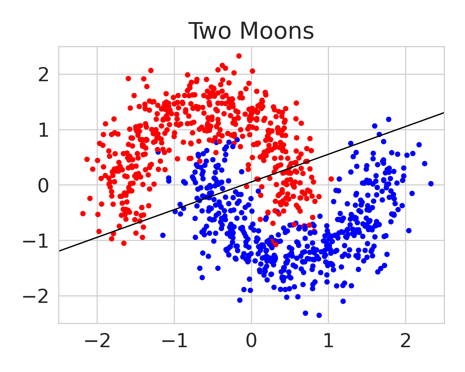
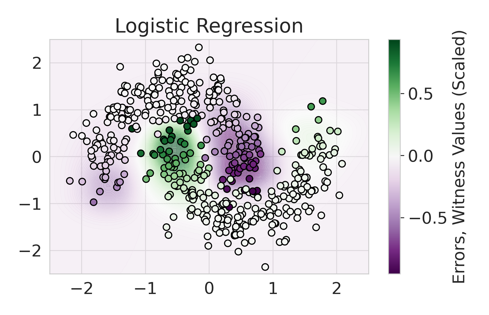
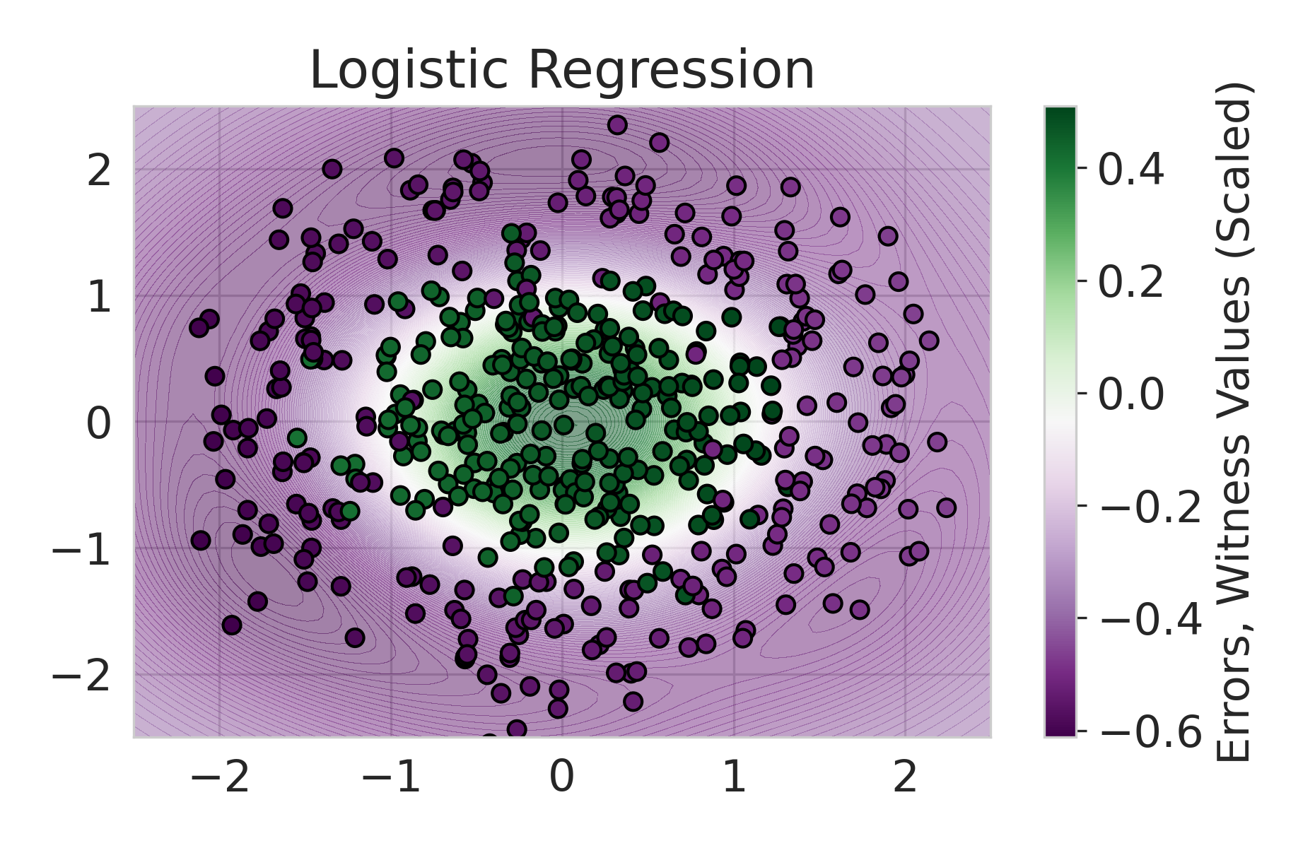
We build on this line of work by considering a more general class of functions given by a Reproducing Kernel Hilbert Space (RKHS), defined on an infinite-dimensional feature space [38]. In fact, an RKHS with a universal kernel is a dense subset of the space of continuous functions [39]. Surprisingly, by leveraging results from information and statistical learning theory [33, 37], we show that the multi-group fairness problem in an RKHS is tractable: the most biased group has a closed form up to a proportionality constant. This leads to an exceedingly simple algorithm (KMAcc, Algorithm 1), which first identifies the function in the RKHS that correlates the most with error $y-f(\boldsymbol{x})$ (called the witness function), and then improves multiaccuracy by subtracting this function from the original predictions. As an example, Figure 1 illustrates that the error of a logistic regression model on the Two Moons synthetic dataset shows a strong correlation with the witness function values.

Refer to caption — Figure 1: Witness function values are highly correlated with errors of the model. Left: Visualization of the moon dataset, with the logistic regression classifier decision boundaries displayed. Middle: Witness function values (Definition 10 with rbf kernel) $c^{\star}_{k,\mathcal{D}_{0},f}$ is plotted as a contour under the error of the classifiers on test samples $y-f(\boldsymbol{x})$ . The colored dots denote the error for each test sample $y-f(x)$ . For samples where the model is most erroneous (dark green and dark purple dots), the predicted witness values are high (dark contour underneath). Right: The error $y-f(x)$ is plotted against the witness values $c^{\star}_{k,\mathcal{D}_{0},f}$ , with a Pearson correlation coefficient of 0.828.

The main contributions of this work include:

1.

We show that multiaccuracy, multicalibration, and outcome indistinguishability are integral probability metrics (IPMs), a well-studied family of statistical distance measures. When the groups or distinguishers lie in an RKHS, these IPMs have closed-form estimators, characterized by a witness function that achieves the supremum.
2.

We introduce a consistent estimator for multiaccuracy, which flags the most discriminated group in terms of a function in Hilbert space, effectively revealing the previously unknown group that suffers the most from inaccurate predictions.
3.

We propose an algorithm, KMAcc (Algorithm 1), which provably corrects the given predictor’s scores against its witness function. Empirically, our algorithm improves multiaccuracy and multicalibration after applying a standard score quantization technique, without the need for the iterative updates required by competing boosting-based models.
4.

We conduct extensive experiments on both synthetic and real-world tabular datasets commonly used in fairness research. We show competitive or improved performance compared to competing models, both in terms of multi-group fairness metrics and AUC.

1.1 Related Literature

Multiaccuracy and Multicalibration.

Multiaccuracy and multicalibration, which emerged from theoretical computer science, ensure fairness over the set of computationally identifiable subgroups [22]. Multiaccuracy aims to make classification errors uncorrelated with subgroups, while multicalibration additionally requires predictions to be calibrated. [22] and [28] ensure multiaccuracy and multicalibration via a two-step process: identify subgroups with accuracy disparities, then apply a transformation to the classification function to boost accuracy over those groups – a method akin to weak agnostic learning [11]. Subsequent works [18, 17, 15] connect multicalibration to the general framework of loss minimization, introducing new techniques including reducing squared multicalibration error and projection-based error corrections [15, 8]. Recent developments include online multicalibration algorithms across Lipschitz convex loss functions [13] and via a game-theoretic approach [20]. In addition, [41] adopts multicalibration for multi-dimensional outputs for fair risk control.

A common thread across work on multigroup fairness is to define subgroups in terms of function classes instead of pre-determined discrete combinations of group-denoting features [28, 9, 18, 29]. Examples of such function classes include “learnable” classes (in the usual statistical learning sense) [28] and the set of indicator functions [10]. Practical implementations of multigroup-fairness ensuring algorithms include MCBoost [28], which uses ridge regression and decision tree regression, and LSBoost [15], which uses linear regression and decision trees. Here, we use both methods as benchmarks. Unlike prior work, we consider the class of functions to be an RKHS and show that this class yields closed-form expressions for the function that correlates the most with error, allowing an efficient multiaccuracy intervention.

Kernel-Based Calibration Metrics.

Calibration ensures that probabilistic predictions are neither over- nor under-confident [40]. Prior works have formulated calibration errors for tasks such as classification [7, 34], regression [36], and beyond [40]. Calibration constraints may be directly incorporated into the training objective of a model [30]. [30, 39, 32, 6] have adopted RKHS as the class of functions to ensure calibration. We build on this prior work and develop kernel-based metrics and consistent estimators focused on multi-group fairness.

Integral Probability Measures (IPMs).

[9] introduces outcome indistinguishability to unify multiaccuracy, multicalibration through a pseudo-randomness perspective – whether one can(not) tell apart “Nature’s” and the predictor’s predictions. We provide an alternative unifying perspective through distances between Nature’s and the predictor’s distributions. As discussed in [9], outcome indistinguishability is closely connected to statistical distance (total variation distance), which, in turn, is one instantiation of an IPM [33], an extensively studied concept in statistical theory that measures the distance between two distributions with respect to a class of functions. [37] provides estimators for IPM defined on various classes of functions, which we apply to develop a consistent estimator for multiaccuracy.

1.2 Notation

We consider a pair of random variables $\boldsymbol{X}$ and $Y$ , taking values in $\mathcal{X}$ and $\mathcal{Y}$ respectively, where $\mathcal{X}$ denotes the input features space to a prediction task and $\mathcal{Y}\subset\mathbb{R}$ the output space. Often, we will take $\mathcal{Y}=\{0,1\}$ , i.e., binary prediction. The pair $(\boldsymbol{X},Y)$ is distributed according to a fixed unknown joint distribution (Nature’s distribution) $P_{\boldsymbol{X},Y}$ with marginals $P_{\boldsymbol{X}}$ and $P_{Y}$ . In binary prediction, we refer to a measurable function $f:\mathcal{X}\to[0,1]$ as a predictor. The predictor $f$ gives rise to a conditional distribution $Q_{Y\mid\boldsymbol{X}=\boldsymbol{x}}(1)\coloneqq f(\boldsymbol{x})$ . We think of $Q_{Y\mid\boldsymbol{X}}$ as an estimate of Nature’s distribution, i.e., $Q_{Y\mid\boldsymbol{X}=\boldsymbol{x}}(1)\approx P_{Y\mid\boldsymbol{X}=% \boldsymbol{x}}(1)$ . The induced joint distribution for $Q_{Y\mid\boldsymbol{X}=\boldsymbol{x}}$ is denoted by $Q_{\boldsymbol{X},Y}\coloneqq P_{\boldsymbol{X}}Q_{Y\mid\boldsymbol{X}}$ ; this joint distribution $Q_{\boldsymbol{X},Y}$ will be referred to as the predictor’s distribution. The marginal distribution $P_{\boldsymbol{X}}$ is the same for both $Q_{\boldsymbol{X},Y}$ and $P_{\boldsymbol{X},Y}$ ; only the conditional distribution $Q_{Y|\boldsymbol{X}}$ changes due to using $f$ .

Given a measurable function $c$ and a random variable $Z\sim P$ , we interchangeably denote expectation by $\mathbb{E}_{P}[c]=\mathbb{E}[c(Z)]=\mathbb{E}_{Z\sim P}[c(Z)]\coloneqq\int_{% \mathcal{Z}}c(z)dP(z)$ depending on what is clearer from context. If $\mathcal{D}$ is a finite set of i.i.d. samples, then we denote the empirical average by $\mathbb{E}_{\mathcal{D}}[c]=\mathbb{E}_{Z\sim\mathcal{D}}[c(Z)]\coloneqq|% \mathcal{D}|^{-1}\sum_{z\in\mathcal{D}}c(z)$ .

2 Multi-Group Fairness as Integral Probability Metrics

We show the connection between IPMs [33, 37] – a concept rooted in statistical learning theory – and multi-group fairness notions such as multiaccuracy, multicalibration [22], and outcome indistinguishability [10]. The key property allowing for these connections is that the multi-group fairness notions and IPMs are both variational forms of measures of deviation between probability distributions. IPMs give perhaps the most general form of such variational representations, and we recall the definition next.

Definition 1 (Integral Probability Metric [33, 37]).

Given two probability measures $P$ and $Q$ supported on $\mathcal{Z}$ and a collection of functions $\mathfrak{C}\subset\{c:\mathcal{Z}\to\mathbb{R}\}$ . We define the integral probability metric (IPM) between $P$ and $Q$ with respect to $\mathfrak{C}$ by

\displaystyle\gamma_{\mathfrak{C}}(P,Q)

\displaystyle\coloneqq\sup_{c\in\mathfrak{C}}\ \left|\mathbb{E}_{Z\sim P}\left% [c(Z)\right]-\mathbb{E}_{Z\sim Q}\left[c(Z)\right]\right|.

(1)

Example 2.

IPMs recover other familiar metrics on probability measures, such as the total variation (statistical distance) metric. Indeed, when $\mathfrak{C}$ is the unit $L^{\infty}$ ball of real-valued functions, i.e., $\mathfrak{C}=\{c:\mathcal{Z}\to\mathbb{R}\ :\ \sup_{z\in\mathcal{Z}}\ |c(z)|% \leq 1\}$ , then $\gamma_{\mathfrak{C}}(P,Q)=\mathsf{TV}(P,Q)$ .

As the example above shows, the complete freedom in choosing the set $\mathfrak{C}$ allows IPMs the ability to subsume existing metrics on probability measures. We show that the expressiveness of IPMs carries through to multi-group fairness notions. Later, in Section 3, we instantiate our IPM framework for multiaccuracy to the particular case when $\mathfrak{C}$ is the unit ball in an infinite-dimensional Hilbert space, which then recovers another familiar metric on probability measures called the maximum mean discrepancy (MMD) or kernel distance.

2.1 Multi-group Fairness Notions

We recall the definitions of multiaccuracy and multicalibration from [28, 29], where the guarantees are parametrized by a class of real-valued functions $\mathfrak{C}\subset\{c:\mathcal{X}\to\mathbb{R}\}$ . We call $\mathfrak{C}$ herein the set of calibrating functions. Intuitively, multi-group notions ensure that $c(\boldsymbol{X})$ for every group-denoting function $c\in\mathfrak{C}$ is uncorrelated with a model’s errors $Y-f(\boldsymbol{X})$ .

Definition 3 (Multiaccuracy [28, 29]).

Fix a collection of functions²²2The range is $[-1,1]$ in [28] and $\mathbb{R}^{+}$ in [29]. We extend the range to $\mathbb{R}$ . $\mathfrak{C}\subset\{c:\mathcal{X}\to\mathbb{R}\}$ and a distribution $P_{\boldsymbol{X},Y}$ supported on $\mathcal{X}\times\mathcal{Y}$ . A predictor $f:\mathcal{X}\to[0,1]$ is ( $\mathfrak{C},\alpha$ )-multiaccurate over $P_{\boldsymbol{X},Y}$ if for all $c\in\mathfrak{C}$ the following inequality holds:

\mu(c,f,P_{\boldsymbol{X},Y})\coloneqq\left|\mathbb{E}\left[c(\boldsymbol{X})(% f(\boldsymbol{X})-Y)\right]\right|\leq\alpha

(2)

Multicalibration proposed by [22] requires the predictor to be unbiased and calibrated against groups denoted by functions in $\mathfrak{C}$ .

Definition 4 (Multicalibration [22, 29, 8]).

Fix a collection of functions $\mathfrak{C}\subset\{c:\mathcal{X}\times[0,1]\to\mathbb{R}\}$ and a distribution $P_{\boldsymbol{X},Y}$ supported on $\mathcal{X}\times\mathcal{Y}$ . Fix a predictor $f:\mathcal{X}\to[0,1]$ such that $f(\boldsymbol{X})$ is a discrete random variable.³³3Alternatively, one can consider a quantization of $f(\boldsymbol{X})$ such as done in [14]. We say that $f$ is ( $\mathfrak{C},\alpha$ )-multicalibrated over $P_{\boldsymbol{X},Y}$ if for all $c\in\mathfrak{C}$ and $v\in\mbox{supp}(f(\boldsymbol{X}))$ :

\left|\mathbb{E}\left[c(\boldsymbol{X},f(\boldsymbol{X}))(f(\boldsymbol{X})-Y)% \mid f(\boldsymbol{X})=v\right]\right|\leq\alpha

(3)

As discussed in [9], multi-group fairness constraints are equivalent to a broader framework of learning called outcome indistinguishability (OI). The object of interest is the distance between the two distributions – the ones induced by the predictor and by Nature.

Definition 5 (Outcome Indistinguishability [9, 10]).

Fix a collection of functions $\mathfrak{C}\subseteq\{c:\mathcal{X}\times[0,1]\times\mathcal{Y}\to\mathbb{R}\}$ and a distribution $P_{\boldsymbol{X},Y}$ supported on $\mathcal{X}\times\mathcal{Y}$ . We say that a predictor $f:\mathcal{X}\to[0,1]$ is ( $\mathfrak{C},\alpha)$ -outcome-indistinguishable if for all $c\in\mathfrak{C}$ ,

\displaystyle\left|\mathbb{E}_{(\boldsymbol{X},Y)\sim P_{\boldsymbol{X},Y}}% \left[c(\boldsymbol{X},f(\boldsymbol{X}),Y)\right]-\mathbb{E}_{(\boldsymbol{X}% ,Y)\sim Q_{\boldsymbol{X},Y}}\left[c(\boldsymbol{X},f(\boldsymbol{X}),Y)\right% ]\right|\leq\alpha,

where we define the induced distribution by the predictor $Q_{\boldsymbol{X},Y}\coloneqq P_{\boldsymbol{X}}Q_{Y\mid\boldsymbol{X}}$ for $Q_{Y\mid\boldsymbol{X}}(1)\coloneqq f(1)$ .

Total Variation (statistical) distance, one instantiation of an IPM [33], provides sufficient conditions for OI ([9]). We establish this broader connection next.

2.2 Equivalence Between Multi-group Fairness Notions and IPMs

Since multiaccuracy, multicalibration, and outcome indistinguishability all pertain to finding the largest distance between distributions with respect to a collection of functions, we can unify them in terms of IPMs. First, we show that ensuring a predictor’s multiaccuracy with respect to a set of calibrating functions $\mathfrak{C}$ is equivalent to ensuring an upper bound on the IPM between Nature’s and the predictor’s distribution with respect to a modified set of function $\widetilde{\mathfrak{C}}$ , given explicitly in the following result.

Proposition 6 (Multiaccuracy as an IPM).

Fix a collection of functions $\mathfrak{C}\subset L^{1}(\mathcal{X})$ , and let $\mathcal{Y}=\{0,1\}$ . Fix a predictor $f:\mathcal{X}\to[0,1]$ inducing the distribution $Q_{\boldsymbol{X},Y}$ . Denote the modified set of functions

\widetilde{\mathfrak{C}}=\left\{\widetilde{c}:\mathcal{X}\times\mathcal{Y}\to% \mathbb{R}\leavevmode\nobreak\ \middle|\leavevmode\nobreak\ \widetilde{c}(% \boldsymbol{x},y)=(-1)^{1-y}\cdot c(\boldsymbol{x})/2\leavevmode\nobreak\ % \mbox{for }c\in\mathfrak{C}\right\}.

(4)

Then, for any $\alpha\geq 0$ , the predictor $f$ is ( $\mathfrak{C},\alpha$ )-multiaccurate if and only if the IPM between Nature’s distribution and the predictor’s distribution is upper bounded by $\alpha$ :

\gamma_{\widetilde{\mathfrak{C}}}(P_{\boldsymbol{X},Y},Q_{\boldsymbol{X},Y})% \leq\alpha.

(5)

Proof.

Let $(\boldsymbol{\xi},Y)$ be an identical copy of $(\boldsymbol{X},Y)$ . Using the notation in (2) in the definition of multiaccuracy (Definition 3), we have that for every $c\in\mathfrak{C}$

$\displaystyle\mu(c,f,P_{\boldsymbol{X},Y})$	$\displaystyle=\left\|\mathbb{E}\left[c(\boldsymbol{\xi})(f(\boldsymbol{\xi})-Y)% \right]\right\|$	(6)
	$\displaystyle=\left\|\mathbb{E}\left[\mathbb{E}\left[c(\boldsymbol{\xi})(Y-f(% \boldsymbol{\xi}))\mid\boldsymbol{\xi}\right]\right]\right\|$	(7)
	$\displaystyle=\left\|\mathbb{E}\left[c(\boldsymbol{\xi})\left(P_{Y\mid% \boldsymbol{X}=\boldsymbol{\xi}}(1)-Q_{Y\mid\boldsymbol{X}=\boldsymbol{\xi}}(1% )\right)\right]\right\|$	(8)
	$\displaystyle=\left\|\mathbb{E}\left[\frac{c(\boldsymbol{\xi})}{2}P_{Y\mid% \boldsymbol{X}=\boldsymbol{\xi}}(1)-\frac{c(\boldsymbol{\xi})}{2}P_{Y\mid% \boldsymbol{X}=\boldsymbol{\xi}}(0)\right]\right.$	(9)
	$\displaystyle\quad\quad\left.-\mathbb{E}\left[\frac{c(\boldsymbol{\xi})}{2}Q_{% Y\mid\boldsymbol{X}=\boldsymbol{\xi}}(1)-\frac{c(\boldsymbol{\xi})}{2}Q_{Y\mid% \boldsymbol{X}=\boldsymbol{\xi}}(0)\right]\right\|$	(10)
	$\displaystyle=\left\|\mathbb{E}_{P_{\boldsymbol{X},Y}}\left[\widetilde{c}\right% ]-\mathbb{E}_{Q_{\boldsymbol{X},Y}}\left[\widetilde{c}\right]\right\|,$	(11)

where $\widetilde{c}(\boldsymbol{x},y)\coloneqq(-1)^{1-y}\cdot c(\boldsymbol{x})/2$ . By definition of multiaccuracy, we have that $f$ is $(\mathfrak{C},\alpha)$ -multiaccurate if and only if $\sup_{c\in\mathfrak{C}}\ \mu(c,f,P_{\boldsymbol{X},Y})\leq\alpha$ . This is equivalent, by the above, to having the IPM bound $\gamma_{\widetilde{\mathfrak{C}}}(P_{\boldsymbol{X},Y},Q_{\boldsymbol{X},Y})\leq\alpha$ , where $\widetilde{\mathfrak{C}}$ is as defined in the proposition statement, i.e., it is the collection of modified functions $\widetilde{c}$ as $c$ ranges over $\mathfrak{C}$ . $\hfill\blacktriangleleft$

Expressing multiaccuracy as an IPM bound will allow us to rigorously accomplish two goals: 1) quantifying multiaccuracy from finitely many samples of $P_{\boldsymbol{X},Y}$ , and 2) correcting a given predictor $f$ to be multiaccurate. These two goals are the subject of Section 3. Similarly, multicalibration and OI can be expressed as IPMs.

Proposition 7 (Multicalibration as an IPM).

Fix a collection of functions $\mathfrak{C}\subseteq\{c:\mathcal{X}\to\mathbb{R}\}$ , and let $\mathcal{Y}=\{0,1\}$ . Fix a predictor $f:\mathcal{X}\to[0,1]$ inducing the distribution $Q_{\boldsymbol{X},Y}$ . Moreover, let $\eta_{y}\coloneqq(-1)^{1-y}$ . Let $d:[0,1]\to\mathcal{V}\subset[0,1]$ , $\left|\mathcal{V}\right|<\infty$ be a discrete, finite quantization of $[0,1]$ , where $P_{\boldsymbol{X}}(d(f(\boldsymbol{X}))=v)>0$ for all $v\in\mathcal{V}$ . Define the set of functions

\widetilde{\mathfrak{C}}_{v}\coloneqq\left\{\widetilde{c}:\mathcal{X}\times% \mathcal{Y}\times\mathcal{V}\to\mathbb{R}\leavevmode\nobreak\ \middle|% \leavevmode\nobreak\ \widetilde{c}(\boldsymbol{x},y,v)=\frac{c(\boldsymbol{x})% \mathds{1}_{f(\boldsymbol{X})=v}\eta_{y}}{2P_{\boldsymbol{X}}(f(\boldsymbol{X}% )=v)}\leavevmode\nobreak\ \mbox{for some }c\in\mathfrak{C}\right\}.

Then $f$ is ( $\mathfrak{C},\alpha$ )-multicalibrated if and only if $\gamma_{\widetilde{\mathfrak{C}}_{v}}(P_{\boldsymbol{X},Y},Q_{\boldsymbol{X},Y% })\leq\alpha$ for every $v\in\mathcal{V}$ .

Proof.

Let $(\boldsymbol{\xi},Y)$ be an identical copy of $(\boldsymbol{X},Y)$ . Using the notation in the definition of multicalibration (Definition 4), we have that for every $c\in\mathfrak{C}$ , $v\in\mathcal{V}$

	$\displaystyle\mathbb{E}\left[c(\boldsymbol{\xi})(Y-f(\boldsymbol{\xi}))\|f(% \boldsymbol{\xi})=v\right]$	(12)
$\displaystyle=$	$\displaystyle\mathbb{E}\left[\frac{c(\boldsymbol{\xi})\mathds{1}_{f(% \boldsymbol{\xi})=v}}{P_{\boldsymbol{X}}(f(\boldsymbol{\xi})=v)}(P_{Y\|% \boldsymbol{X}=\boldsymbol{\xi}}(1)-Q_{Y\|\boldsymbol{X}=\boldsymbol{\xi}}(1))\right]$	(13)
$\displaystyle=$	$\displaystyle\mathbb{E}\left[\frac{c(\boldsymbol{\xi})\mathds{1}_{f(% \boldsymbol{\xi})=v}}{2P_{\boldsymbol{X}}(f(\boldsymbol{\xi})=v)}(P_{Y\|% \boldsymbol{X}=\boldsymbol{\xi}}(1)-P_{Y\|\boldsymbol{X}=\boldsymbol{\xi}}(0))\right]$	(14)
	$\displaystyle\quad-\mathbb{E}\left[\frac{c(\boldsymbol{\xi})\mathds{1}_{f(% \boldsymbol{\xi})=v}}{2P_{\boldsymbol{X}}(f(\boldsymbol{\xi})=v)}(Q_{Y\|% \boldsymbol{X}=\boldsymbol{\xi}}(1)-Q_{Y\|\boldsymbol{X}=\boldsymbol{\xi}}(0))\right]$	(15)
$\displaystyle=$	$\displaystyle\mathbb{E}_{P_{\boldsymbol{X},Y}}\left[\widetilde{c}\right]-% \mathbb{E}_{Q_{\boldsymbol{X},Y}}\left[\widetilde{c}\right]$	(16)

where $\displaystyle\widetilde{c}(\boldsymbol{x},y,v)\coloneqq\frac{c(\boldsymbol{x})% \mathds{1}_{f(\boldsymbol{X})=v}\eta_{y}}{2P_{\boldsymbol{X}}(f(\boldsymbol{X}% )=v)}$ . $\hfill\blacktriangleleft$

Proposition 8 (OI as an IPM).

Let $\mathfrak{C}\subset\{c:\mathcal{X}\times[0,1]\times\{0,1\}\to\mathbb{R}\}$ be a collection of functions, and fix a predictor $f:\mathcal{X}\to[0,1]$ inducing the distribution $Q_{\boldsymbol{X},Y}$ on $\mathcal{X}\times\{0,1\}$ via composing with $P_{\boldsymbol{X}}$ . Define the set of function

\widetilde{\mathfrak{C}}=\left\{\widetilde{c}:\mathcal{X}\times\{0,1\}\to% \mathbb{R}\mid\widetilde{c}(\boldsymbol{x},y)=c(\boldsymbol{x},f(\boldsymbol{x% }),y)\text{ for some }c\in\mathfrak{C}\right\}.

(17)

Then, for any $\alpha\geq 0$ , $f$ is ( $\mathfrak{C},\alpha$ )-OI if and only if $\gamma_{\widetilde{\mathfrak{C}}}(P_{\boldsymbol{X},Y},Q_{\boldsymbol{X},Y})% \leq\alpha.$

Proof.

From Definition 1, if $\gamma_{\widetilde{\mathfrak{C}}}(P_{\boldsymbol{X},Y},Q_{\boldsymbol{X},Y})\leq\alpha$ ,

$\displaystyle\gamma_{\widetilde{\mathfrak{C}}}(P_{\boldsymbol{X},Y},Q_{% \boldsymbol{X},Y})\coloneqq$	$\displaystyle\sup_{\widetilde{c}\in\widetilde{\mathfrak{C}}}\ \left\|\mathbb{E}% _{(\boldsymbol{X},Y)\sim P_{\boldsymbol{X},Y}}\left[\widetilde{c}(\boldsymbol{% X},Y)\right]-\mathbb{E}_{(\boldsymbol{X},Y)\sim Q_{\boldsymbol{X},Y}}\left[% \widetilde{c}(\boldsymbol{X},Y)\right]\right\|$	(18)
	$\displaystyle=\sup_{c\in\mathfrak{C}}\ \left\|\mathbb{E}_{(\boldsymbol{X},Y)% \sim P_{\boldsymbol{X},Y}}\left[c(\boldsymbol{X},f(\boldsymbol{X}),Y)\right]\right.$	(19)
	$\displaystyle\quad\left.-\mathbb{E}_{(\boldsymbol{X},Y)\sim Q_{\boldsymbol{X},% Y}}\left[c(\boldsymbol{X},f(\boldsymbol{X}),Y)\right]\right\|$	(20)
	$\displaystyle\leq\alpha$	(21)

By Definition 5, $f$ is ( $\mathfrak{C},\alpha$ )-OI. The other direction is analogous. $\hfill\blacktriangleleft$

3 Multiaccuracy in Hilbert Space

We develop a theoretical framework and an algorithm for quantifying and ensuring $(\mathfrak{C},\alpha)$ -multiaccuracy. We consider the group-denoting functions $\mathfrak{C}_{k}$ to be the unit ball in an infinite-dimensional Hilbert space, namely, an RKHS $\mathcal{H}_{k}$ defined by a given kernel $k$ (Definition 9). The proposed set of calibration functions $\mathfrak{C}_{k}$ can easily exhibit and exceed the expressivity of group-denoting indicator functions. Surprisingly, despite the expressiveness of $\mathfrak{C}_{k}$ , we show that the calibration function that maximizes multiaccuracy error, i.e. the witness function $c_{k}^{\star}$ (Definition 10), has a closed form – in contrast to when $\mathfrak{C}$ is, for example, a set of decision trees [15, 28]. This enables us to derive a procedure for ensuring multiaccuracy (KMAcc, Algorithm 1).

3.1 Calibration Functions in RKHS and its Witness Function for Multiaccuracy

Our choice of calibrating functions $\mathfrak{C}$ is the set of functions with bounded norm in an RKHS. First, recall that an RKHS can be defined via kernal functions, as follows⁴⁴4The characterizing property of a real RKHS is that it is a Hilbert space $\mathcal{H}$ of functions $c:\mathcal{X}\to\mathbb{R}$ for which every evaluation map $c\mapsto c(\boldsymbol{x})$ is a continuous function from $\mathcal{H}$ to $\mathbb{R}$ for each fixed $\boldsymbol{x}\in\mathcal{X}$ ..

Definition 9 (Reproducing kernel Hilbert space (RKHS)).

Let $\mathcal{H}\subset\{c:\mathcal{X}\to\mathbb{R}\}$ be a real Hilbert space with inner product $\langle\,\cdot\,,\,\cdot\,\rangle_{\mathcal{H}}$ , and fix a function $k:\mathcal{X}^{2}\to\mathbb{R}$ . We say that $\mathcal{H}$ is a reproducing kernel Hilbert space with kernel $k$ if it holds that $k(\,\cdot\,,\boldsymbol{x})\in\mathcal{H}$ for all $\boldsymbol{x}\in\mathcal{X}$ and $\langle c,k(\,\cdot\,,\boldsymbol{x})\rangle_{\mathcal{H}}=c(\boldsymbol{x})$ for all $c\in\mathcal{H}$ and $\boldsymbol{x}\in\mathcal{X}$ . We denote $\mathcal{H}$ by $\mathcal{H}_{k}$ if $k$ is given.

We use the structure of the RKHS as our group-denoting functions. Thus, for a prescribed multiaccuracy level $\alpha$ , we will need to restrict attention to elements of $\mathcal{H}_{k}$ whose norm satisfies a given bound. To normalize, we choose the unit ball in $\mathcal{H}_{k}$ as our set of calibration functions, i.e.

\mathfrak{C}_{k}\coloneqq\left\{c\in\mathcal{H}_{k}\ :\ \|c\|_{\mathcal{H}_{k}% }\ \leq 1\right\}.

(22)

We note that when the class of functions $\mathfrak{C}$ is the unit ball in an RKHS, the induced IPM $\gamma_{\mathfrak{C}}(P,Q)$ is called the maximum mean discrepancy (MMD) [37].

Of particular importance are calibration functions $c\in\mathfrak{C}$ that attain the maximal multiaccuracy error (the LHS of (2)). Such functions, called witness functions [27], encode the multiaccuracy definition without the need to consider the full set $\mathfrak{C}$ .

Definition 10 (Witness function for multiaccuracy).

For a fixed set of calibration functions $\mathfrak{C}\subset\{c:\mathcal{X}\to\mathbb{R}\}$ , predictor $f:\mathcal{X}\to[0,1]$ , and distribution $P_{\boldsymbol{X},Y}$ , we say that $c^{\star}\in\mathfrak{C}$ is a witness function for multiaccuracy of $f$ with respect to $\mathfrak{C}$ if it attains the maximum on the LHS in (2):

\mu(c^{\star},f,P_{\boldsymbol{X},Y})=\max_{c\in\mathfrak{C}}\ \mu(c,f,P_{% \boldsymbol{X},Y}).

(23)

While an RKHS can encompass a broader class of functions than shallow decision trees or linear models, finding the function in the RKHS that errs the most (i.e., the witness function as per Definition 10) is surprisingly simple. Firstly, it can be shown that for the IPM $\gamma_{\mathfrak{C}_{k}}(P,Q)$ (where $\mathfrak{C}_{k}$ is the unit ball in $\mathcal{H}_{k}\subset\{c:\mathcal{Z}\to\mathbb{R}\}$ ), the function $c\in\mathfrak{C}_{k}$ that maximizes the RHS of (1) is in closed form, up to a multiplicative constant [19, 27]

c^{\star}(z)\propto\mathbb{E}_{\zeta\sim P}\left[k(z,\zeta)\right]-\mathbb{E}_% {\zeta\sim Q}\left[k(z,\zeta)\right].

(24)

By the connection between IPM and multiaccuracy, we can similarly find the closed form of the witness function for multiaccuracy(Definition 10).

Proposition 11 (Witness function for multiaccuracy).

Given a the kernel function $k:\mathcal{X}^{2}\to\mathbb{R}$ and distribution $P_{\boldsymbol{X},Y}$ over $\mathcal{X}\times\{0,1\}$ . We assume that $\mathcal{H}_{k}\subset L^{1}(\mathcal{X})$ ⁵⁵5 $L^{1}(\mathcal{X})$ denotes the space of real-valued functions that are integrable against $P_{\boldsymbol{X}}$ , i.e. $L^{1}(\mathcal{X})\coloneqq\left\{c:\mathcal{X}\to\mathbb{R}\ :\ \mathbb{E}% \left[\left|c(\boldsymbol{X})\right|\right]<\infty\right\}$ .. Fix a predictor $f:\mathcal{X}\to[0,1]$ satisfying $\mathbb{E}[k(\,\cdot\,,\boldsymbol{X})f(\boldsymbol{X})]\in\mathcal{H}_{k}$ . Then, there exists a unique (up to sign) witness function for multiaccuracy of $f$ with respect to $\mathfrak{C}_{k}$ (as per Definition 10), and it is given by

c_{k,f}^{\star}(\boldsymbol{x})\coloneqq\mathbb{E}\left[\theta\cdot(Y-f(% \boldsymbol{X}))k(\boldsymbol{x},\boldsymbol{X})\right],

(25)

where $\theta\in\mathbb{R}$ is a normalizing constant so that $\|c_{k,f}^{\star}\|_{\mathcal{H}_{k}}=1$ .

Proof.

First, by continuity of the evaluation functionals on $\mathcal{H}_{k}$ , we obtain that $h_{n}(\boldsymbol{x})\coloneqq\sum_{i=1}^{n}c_{i}k(\boldsymbol{x}_{i},% \boldsymbol{x})\to c(\boldsymbol{x})$ pointwise for each $\boldsymbol{x}\in\mathcal{X}$ as $n\to\infty$ [4, Chapter 1, Corollary 1]. Let $h(\boldsymbol{x})\coloneqq\sum_{i=1}^{\infty}|c_{i}k(\boldsymbol{x}_{i},% \boldsymbol{x})|$ . Next, applying Proposition 6, $(\mathfrak{C}_{k},\alpha)$ -multiaccuracy of $f$ is equivalent to the IPM bound $\gamma_{\widetilde{\mathfrak{C}}}(P_{\boldsymbol{X},Y},Q_{\boldsymbol{X},Y})\leq\alpha$ , where $\widetilde{\mathfrak{C}}$ and $Q_{\boldsymbol{X},Y}$ are as constructed in Proposition 6. Next, we use the definition of IPMs to deduce the formula for the witness function.

We rewrite the function inside the maximization definition of $\gamma_{\widetilde{\mathfrak{C}}}(P_{\boldsymbol{X},Y},Q_{\boldsymbol{X},Y})$ as an inner product in $\mathcal{H}$ . Fix $c$ as above. Then, with $\widetilde{c}(\boldsymbol{x},y)\coloneqq(-1)^{1-y}c(\boldsymbol{x})/2$ , we have that

$\displaystyle 2\mathbb{E}_{P_{\boldsymbol{X},Y}}[\widetilde{c}]$	$\displaystyle=\mathbb{E}_{P_{\boldsymbol{X},Y}}\left[(-1)^{1-Y}c(\boldsymbol{X% })\right]$	(26)
	$\displaystyle=\mathbb{E}_{P_{\boldsymbol{X},Y}}\left[(-1)^{1-Y}\left\langle c,% k(\,\cdot\,,\boldsymbol{X})\right\rangle_{\mathcal{H}}\right]$	(27)
	$\displaystyle=\mathbb{E}_{P_{\boldsymbol{X},Y}}\left[(-1)^{1-Y}\langle\sum_{i% \in\mathbb{N}}c_{i}k(\boldsymbol{x}_{i},\,\cdot\,),k(\,\cdot\,,\boldsymbol{X})% \rangle_{\mathcal{H}}\right]$	(28)
	$\displaystyle=\mathbb{E}_{P_{\boldsymbol{X},Y}}\left[(-1)^{1-Y}\sum_{i\in% \mathbb{N}}c_{i}\langle k(\boldsymbol{x}_{i},\,\cdot\,),k(\,\cdot\,,% \boldsymbol{X})\rangle_{\mathcal{H}}\right]$	(29)
	$\displaystyle=\sum_{i\in\mathbb{N}}c_{i}\ \mathbb{E}_{P_{\boldsymbol{X},Y}}% \left[(-1)^{1-Y}k(\boldsymbol{x}_{i},\boldsymbol{X})\right],$	(30)

where (29) follows by continuity of the inner product and (30) by Fubini’s theorem since $\mathcal{H}_{k}\subset L^{1}(\mathcal{X})$ . The same steps follow for $Q_{\boldsymbol{X},Y}$ in place of $P_{\boldsymbol{X},Y}$ , and subtracting the ensuing two equations we obtain

	$\displaystyle\mathbb{E}_{P_{\boldsymbol{X},Y}}[\widetilde{c}]-\mathbb{E}_{Q_{% \boldsymbol{X},Y}}[\widetilde{c}]$	$\displaystyle=\sum_{i\in\mathbb{N}}c_{i}\mathbb{E}_{P_{\boldsymbol{X},Y}}\left% [(Y-f(\boldsymbol{X}))k(\boldsymbol{x}_{i},\boldsymbol{X})\right]$		(31)
		$\displaystyle=\langle c,\mathbb{E}_{P_{\boldsymbol{X},Y}}\left[(Y-f(% \boldsymbol{X}))k(\,\cdot\,,\boldsymbol{X})\right]\rangle_{\mathcal{H}}.$		(32)

Therefore, the maximizing function is given up to a normalizing constant by

c_{k,f}^{\star}(\boldsymbol{x})\propto\mathbb{E}_{P_{\boldsymbol{X},Y}}\left[(% Y-f(\boldsymbol{X}))k(\boldsymbol{x},\boldsymbol{X})\right].\

$\hfill\blacktriangleleft$

In the presence of finitely many samples, one must resort to numerical approximations of the witness function.

Definition 12 (Empirical Witness Function).

Let $\mathcal{D}_{0}$ be a finite set of i.i.d. samples from $P_{\boldsymbol{X},Y}$ . We define the empirical witness function as the plug-in estimator of (25):

c_{k,\mathcal{D}_{0},f}^{\star}(\boldsymbol{x})=\mathbb{E}_{(\boldsymbol{X},Y)% \sim\mathcal{D}_{0}}\left[\hat{\theta}\cdot(Y-f(\boldsymbol{X}))k(\boldsymbol{% x},\boldsymbol{X})\right],

(33)

where $\hat{\theta}\in\mathbb{R}$ is a normalizing constant so that $\|c_{k,\mathcal{D}_{0},f}^{\star}\|_{\mathcal{H}}=1$ .

Observe that given a training dataset $\{\boldsymbol{x}_{i}\}_{i=1}^{n}$ , the witness function for a new sample $\boldsymbol{x}$ is proportional to the sum of the error of $\boldsymbol{x}_{i}$ weighted by $k(\boldsymbol{x},\boldsymbol{x}_{i})$ – the distance between $\boldsymbol{x}_{i}$ and the new sample $\boldsymbol{x}$ in the kernel space. The witness function is performing a kernel regression of a model’s errors. From the definition of the witness function, it attains the supremum in the IPM, which measures the distance between Nature and the Predictor’s distribution. Hence, if a new sample $\boldsymbol{x}$ attains a high witness function value, $f(\boldsymbol{x})$ is likely erroneous.

We call the multiaccuracy error when $\mathfrak{C}$ comes from an RKHS the kernel multiaccuracy error, defined with the witness function $c_{k,f}^{\star}(\boldsymbol{X})$ which attains the maximum error.

Definition 13 (Kernel Multiaccuracy Error (KME)).

Let $\mathfrak{C}_{k}$ be the set of calibration functions in the RKHS $\mathcal{H}_{k}$ as defined in (22). Given a predictor $f$ , the kernel multiaccuracy error (KME) is defined as

\displaystyle\gamma_{k}(f,P_{\boldsymbol{X},Y})\coloneqq\left|\mathbb{E}\left[% c_{k,f}^{\star}(\boldsymbol{X})(Y-f(\boldsymbol{X}))\right]\right|.

(34)

The empirical version has the plug-in estimator of the witness function $c_{k,f}^{\star}$ .

Definition 14 (Empirical KME).

Given a test set of freshly sampled i.i.d. datapoints $\mathcal{D}$ , we define the empirical KME by

\displaystyle\gamma_{k}(f,\mathcal{D})\coloneqq\left|\mathbb{E}_{(\boldsymbol{% X},Y)\sim\mathcal{D}}\left[c_{k,\mathcal{D}_{0},f}^{\star}(\boldsymbol{X})(Y-f% (\boldsymbol{X}))\right]\right|.

(35)

$\blacktriangleright$ Remark 15 (Overcoming the Curse of Dimensionality).

One important observation is that the MMD estimator depends on the dataset $\mathcal{D}$ only through the kernel $k$ . Hence, once $k(\boldsymbol{x}_{i},\boldsymbol{x}_{j})$ is known, the complexity of the estimator is independent of the dimensionality of $\boldsymbol{X}$ – e.g., for $\boldsymbol{X}\in\mathbb{R}^{d}$ , sample complexity does not scale exponentially with $d$ (see the end of Section 2.1 in [37]. $\lrcorner$

We give the consistency and rate of convergence of KME – the finite-sample estimation of KME converges to the true expectation, following a direct application of [37, Corollary 3.5].

Theorem 16 (Consistency of the KME Estimator, [37, Corollary 3.5]).

Suppose the kernel $k$ is measurable and satisfies $\sup_{\boldsymbol{x}\in\mathcal{X}}k(\boldsymbol{x},\boldsymbol{x})\leq C<\infty$ . Then, with probability at least $1-2e^{-\tau}$ over the choice of i.i.d. samples $\mathcal{D}$ from $P_{\boldsymbol{X},Y}$ and for every predictor $f:\mathcal{X}\to[0,1]$ , there is a constant $A=A(f,P_{\boldsymbol{X},Y})$ such that the inequality

\displaystyle|\gamma_{k}(f,\mathcal{D})-\gamma_{k}(f,P_{\boldsymbol{X},Y})|% \leq A(\frac{1+\sqrt{\tau}}{\sqrt{|\mathcal{D}|}}+\frac{\tau}{|\mathcal{D}|}),

(36)

In addition, we have the almost-sure convergence $\gamma_{k}(f,\mathcal{D})\rightarrow\gamma_{k}(f,P_{\boldsymbol{X},Y})$ as $|\mathcal{D}|\rightarrow\infty$ .

Next, we proceed to show an algorithm, KMAcc, that corrects a given predictor $f$ of its multiaccuracy error using the empirical witness function.

3.2 KMAcc: Proposed Algorithm for Multiaccuracy

We propose a simple algorithm KMAcc (Algorithm 1) that corrects the original predictor from multiaccuracy error. Notably, KMAcc does not require iterative updates, unlike all competing boosting or projection-based models [28, 15, 8]. In a nutshell, KMAcc first identifies the function in the RKHS that correlates the most with the predictor’s error $y-f(\boldsymbol{x})$ (called the witness function) and subtracts this function from the original prediction to get a multi-group fair model. The first step is surprisingly simple – as we have shown above, the witness function of an RKHS has a closed form up to a proportionality constant. The second step is an additive update followed by clipping.

As outlined in Algorithm 1, the algorithm takes in a pre-trained base predictor $f$ , a proportionality constant $\lambda$ , and a (testing) dataset $\mathcal{D}$ on which the model is evaluated. Additionally, to define the witness function and the RKHS, the algorithm is given a dataset reserved for learning the witness function $\mathcal{D}_{0}$ and a kernel function $k$ . With these, for each sample, the algorithm first computes the witness function value, and subtracts away the witness function value multiplied by $\lambda$ , the proportionality constant which we learn from data (described in the next paragraph). Finally, we clip the output to fall within $[0,1]$ .

Learning the Proportionality Constant.

There are multiple approaches to obtaining the proportionality constant that scales the witness function appropriately. As an example, we adopt a data-driven approach to find $\lambda$ . We use a validation set to perform a grid search on $[0,1]$ to get the $\lambda$ that produces a predictor $g^{\prime}(\boldsymbol{x})=f(\boldsymbol{x})+\lambda c^{\star}_{k,\mathcal{D}_% {0},f}(\boldsymbol{x})$ that is closest to $f$ in terms of $L-2$ distance, while also satisfying a $\alpha-$ multiaccuracy with a specified $\alpha$ ⁶⁶6When the multiaccuracy constraint cannot be met, we output the $\lambda$ that achieves the lowest multiaccuracy error using the witness values of $f$ ..

Algorithm 1 KMAcc.

$\blacktriangleright$ Remark 17 (One-Step Update).

For the linear kernel $k(x,x^{\prime})=x^{T}x^{\prime}$ , we show that KMAcc yields a $0$ -multiaccurate predictor in a single step. While this property does not extend to nonlinear kernels, we observe empirically that the one-step update in KMAcc significantly reduces the empirical KME for RBF kernels. See Appendix C. for a detailed discussion.

We discuss in the following section a theoretical framework that gives rise to KMAcc and the grid-search approach.

3.3 Theoretical Framework for KMAcc

We formulate an optimization that, given a prediction $f:\mathcal{X}\to[0,1]$ that is not necessarily multiaccurate, finds the “closest” predictor $g:\mathcal{X}\to[0,1]$ that is corrected for multiaccuracy with respect to the empirical witness function $c_{k,\mathcal{D}_{0},f}^{\star}$ of $f$ . Specifically, we consider the mean-squared loss to obtain the problem:

	$\displaystyle\underset{g:\mathcal{X}\to[0,1]}{\text{minimize}}$	$\displaystyle\quad\frac{1}{2}\mathbb{E}_{(\boldsymbol{X},Y)\sim\mathcal{D}}% \left[(f(\boldsymbol{X})-g(\boldsymbol{X}))^{2}\right]$		(37)
	subject to	$\displaystyle\quad\left\|\mathbb{E}_{(\boldsymbol{X},Y)\sim\mathcal{D}}\left[c^% {\star}_{k,\mathcal{D}_{0},f}(\boldsymbol{X})(g(\boldsymbol{X})-Y)\right]% \right\|\leq\alpha.$

where $\mathcal{D}_{0}$ and $\mathcal{D}$ are sets of i.i.d. samples that are sampled independently of each other.

A closer look at (37) shows that it is a quadratic program (QP)⁷⁷7Please find details of QP formulation in Appendix A. Thus, we can solve this QP through its dual problem to obtain a closed-form formula for the solution $g^{\star}$ . The following formula follows by applying standard results on QP [5, Chapter 4.4].

Theorem 18.

Fix two independently sampled sets of i.i.d. samples $\mathcal{D}_{0}$ and $\mathcal{D}$ from $P_{\boldsymbol{X},Y}$ with $|\mathcal{D}|=n$ , and let $\boldsymbol{f}=\boldsymbol{f}_{\mathcal{D}}$ , $\boldsymbol{y}=\boldsymbol{y}_{\mathcal{D}}$ , $\boldsymbol{c}=\boldsymbol{c}_{\mathcal{D}_{0},\mathcal{D}}$ , $\boldsymbol{A}=\boldsymbol{A}_{\mathcal{D}_{0},\mathcal{D}}$ and $\boldsymbol{b}=\boldsymbol{b}_{\mathcal{D}_{0},\mathcal{D}}$ be the fixed vectors and matrix as defined in (41)–(44). Denote an optimization variable $\mathcal{L}=(\lambda_{+},\lambda_{-},\boldsymbol{\xi}_{+}^{T},\boldsymbol{\xi}% _{-}^{T})^{T}\in\mathbb{R}^{2n+2}$ and let $\boldsymbol{B}=\frac{1}{2}\boldsymbol{A}\boldsymbol{A}^{T}\in\mathbb{R}^{(2n+2% )\times(2n+2)}$ and $\boldsymbol{d}=\boldsymbol{b}-\boldsymbol{A}\boldsymbol{f}$ . Let $\mathcal{L}^{\star}=(\lambda_{+}^{\star},\lambda_{-}^{\star},(\boldsymbol{\xi}% _{+}^{\star})^{T},(\boldsymbol{\xi}_{-}^{\star})^{T})^{T}$ be the unique solution to the QP

\underset{\mathcal{L}\geq\mathbf{0}}{\textup{minimize}}\ \mathcal{L}^{T}% \boldsymbol{B}\mathcal{L}+\boldsymbol{d}^{T}\mathcal{L}.

(38)

Then, the predictors solving the optimization (37) are determined by their restriction to $\mathcal{D}$ as

g(\boldsymbol{x}_{i})=f(\boldsymbol{x}_{i})+\lambda^{\star}c_{k,\mathcal{D}_{0% },f}^{\star}(\boldsymbol{x}_{i})+\xi_{i}^{\star}

(39)

where $\lambda^{\star}\coloneqq\frac{1}{n}(\lambda_{-}^{\star}-\lambda_{+}^{\star})$ and $\boldsymbol{\xi}^{\star}\coloneqq\boldsymbol{\xi}_{-}^{\star}-\boldsymbol{\xi}% _{+}^{\star}$ . Furthermore, the value of $\boldsymbol{\xi}^{\star}$ may be chosen⁸⁸8To see this, note that, thinking of $\lambda_{-}$ and $\lambda_{+}$ as constants, the optimization over a single pair $(\xi_{-,i},\xi_{+,i})$ takes the form of minimizing $(\xi_{i}+\lambda c_{i})^{2}/2+f_{i}\xi_{i}+\xi_{+,i}$ over $\xi_{+,i}\geq 0$ and $\xi_{i}\geq-\xi_{+,i}$ . The optimal value for this can be easily seen to be $\xi_{i}=-\lambda c_{i}-f_{i}$ if $\lambda c_{i}+f_{i}<0$ , or $\xi_{i}=0$ if $\lambda c_{i}+f_{i}\in[0,1]$ , or $1-\lambda c_{i}-f_{i}$ if $\lambda c_{i}+f_{i}>1$ . This translates to clipping $g$ to be within $[0,1]$ . so that $g$ is projected onto $[0,1]$ . In particular, applying KMAcc (Algorithm 1) with the value $\lambda=\lambda^{\star}$ attains a solution to (37).

4 Experiments

We benchmark our proposed algorithm, KMAcc (Algorithm 1), on four synthetic datasets and eight real-world tabular datasets¹¹¹¹11Implementation of KMAcccan be found at https://github.com/Carol-Long/KMAcc. We demonstrate KMAcc’s competitive or improved performance among competing interventions, both in multi-group fairness metrics and in AUC. Full experimental results are provided in Appendix B.

4.1 Datasets

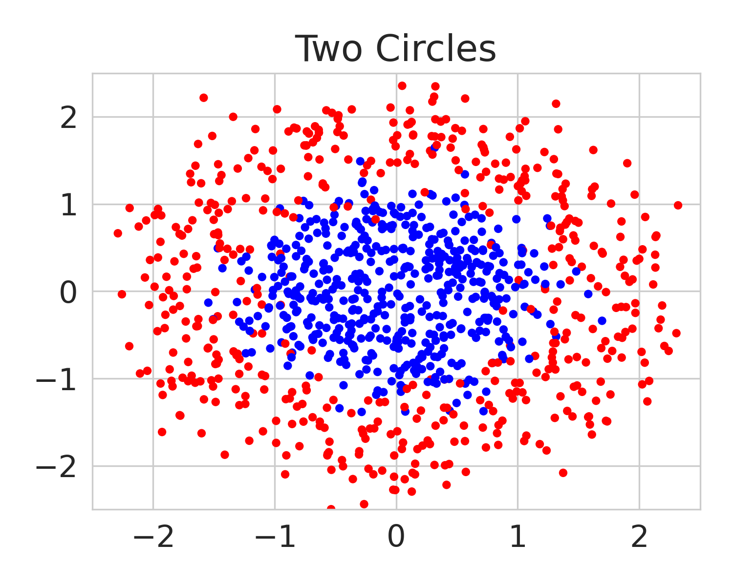
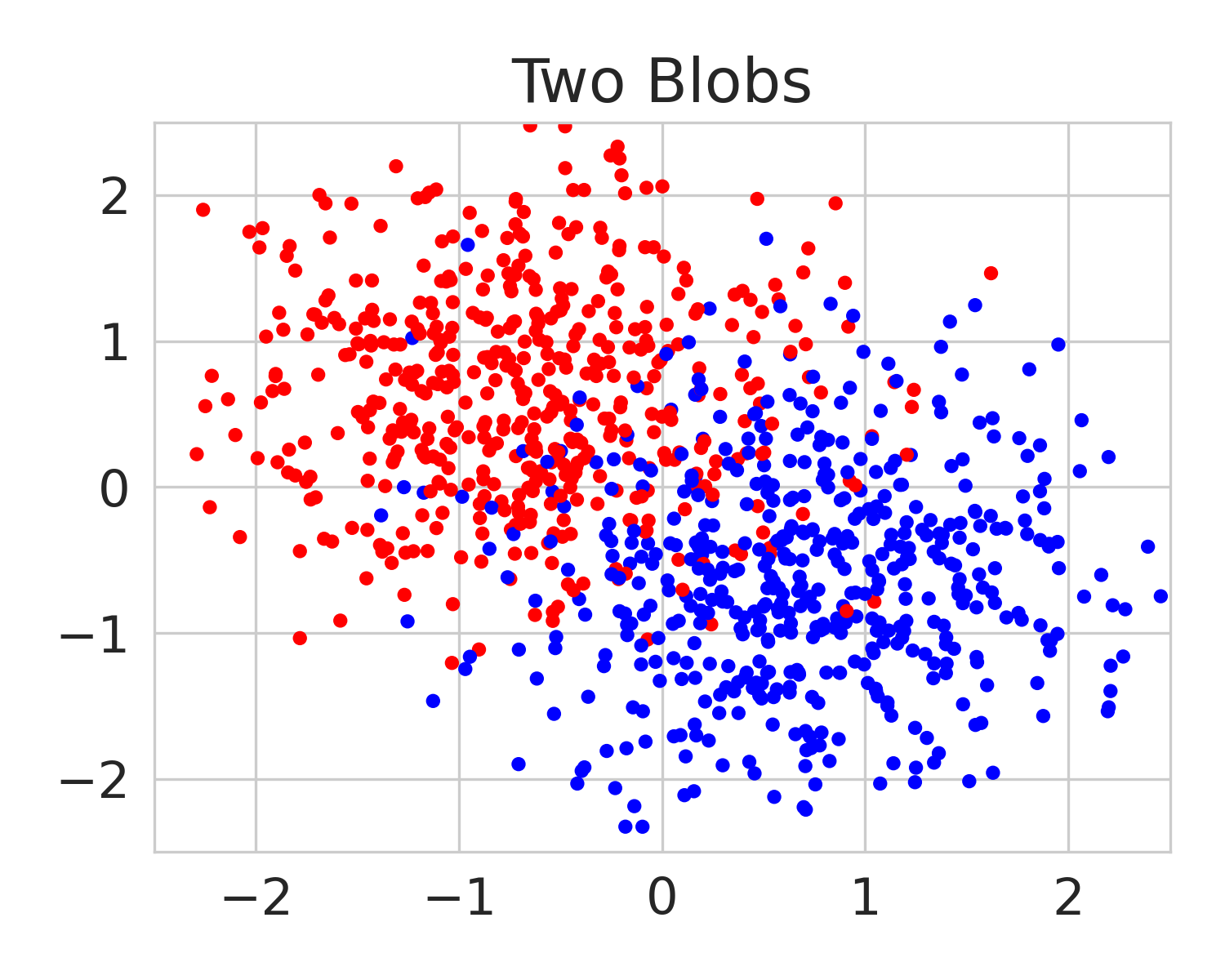
We provide experimental results from the US Census dataset FolkTables. We conduct 4 binary classification tasks, including ACSIncome, ACSPublicCoverage, ACSMobility, ACSEmployment, using two different states for each of these tasks. In addition, we generate four synthetic datasets using the sklearn.datasets class in Scikit-Learn [35] – moons, concentric circles, blobs with varied variance, and anisotropically distributed data.

4.2 Competing Methods

We benchmark our method against LSBoost¹²¹²12We use the official implementation of LSBoost available at https://github.com/Declancharrison/Level-Set-Boosting. by [15] and MCBoost¹³¹³13We use the official implementation of MCBoost available at https://osf.io/kfpr4/?view_only=adf843b070f54bde9f529f910944cd99. by [29], which are (to the best of our knowledge) the two existing algorithms of multi-group fairness with usable Python implementations.

The mechanism of LSBoost is the following: over a number of level set partitions, each called $v$ , LSBoost finds a function $c_{v}^{t+1}\in\mathcal{C}$ through a squared error regression oracle before updating a function $f_{t+1}$ as a rounding of the values to each level set using a successive updating of indicator values as to which set they lie in under the previous $f_{t}$ combined with the learned $c^{t+1}_{v}$ : $\hat{f}=\sum_{v\in[1/m]}\mathbf{1}[f_{t}(x)=v]\cdot c_{v}^{t+1}(x)$ , and $f=\text{Round}(\hat{f}_{t+1},m)$ . This updating continues so long as an error term measured by the expectation of the squared error continues to decrease at a rate above a parameterized value. $\mathcal{C}$ is taken to be linear regression or decision trees.

The MCBoost algorithm performs an iterative multiplicative weights update applied to successively learned functions. Starting with an initial predictor $p_{0}$ , it learns a series of grouping functions $c(x)\in\mathcal{C}$ , that maximize multiaccuracy error. The algorithm now stores a set of both calibration points $S$ and validation points $V$ , at each step generating the set $S_{t}$ by, $\forall(x,y)\in S$ , having $(x,y-p_{t}(x))\in S_{t}$ . Then, using the weak agnostic learner on $S_{t}$ , it produces a function $c$ which has its multiaccuracy checked on the validation set $V$ with the empirical estimate of the multiaccuracy error before enacting a multiplicative weights update $f_{t+1}(\boldsymbol{x})=e^{-\eta h_{t,S}(\boldsymbol{x})}\cdot f_{t}(% \boldsymbol{x})$ if the multiaccuracy error is large. There are three different classes $\cal{C}$ it might draw $c$ from – either taking sub-populations parameterized by some number of intersections of features, using ridge regression, or using shallow decision trees.

4.3 Performance Metrics

We evaluate the performance of baseline and multi-group fair models across three metrics: Kernel Multiaccuracy Error (KME, Definition 13), Area Under the ROC Curve (AUC), and Mean-Squared Calibration Error (MSCE), where MSCE is defined as follows.

Definition 19 (Mean-Squared Calibration Error (MSCE), [15]).

The Mean-Squared Calibration Error (MSCE) over a dataset $\mathcal{D}$ of a predictor $f:\mathcal{X}\to[0,1]$ with a countable range $R(f)$ is defined by

\displaystyle\textup{MSCE}(f,\mathcal{D})\coloneqq\sum_{v\in R(f)}\Pr_{(% \boldsymbol{X},Y)\sim\mathcal{D}}[f(\boldsymbol{X})=v]\cdot\left(\mathbb{E}_{(% \boldsymbol{X},Y)\sim\mathcal{D}}\left[(Y-v)\mid f(\boldsymbol{X})=v\right]% \right)^{2},

Our algorithm optimizes for KME and utility, while LSBoost [15] optimizes for MSCE. Hence, both of these metrics are reported. MCBoost [28] optimizes for multiaccuracy error (without considering calibration functions in the kernel space) and classification accuracy. We report AUC since it captures the models’ performance across all classification thresholds.

4.4 Methodology

To implement and benchmark KMAcc, we proceed through the following steps.

Data splits.

We assume access to a set of i.i.d. samples $\mathcal{D}^{\prime}$ drawn from $P_{\boldsymbol{X},Y}$ , where $P_{\boldsymbol{X},Y}$ is a distribution over $\mathcal{X}\times\mathcal{Y}=\mathbb{R}^{m}\times\{0,1\}$ . We randomly partition $\mathcal{D}^{\prime}$ into four disjoint subsets: $\mathcal{D}_{\text{train}}$ (for training the baseline predictor $f$ ), $\mathcal{D}_{0}$ for computing the witness function $c^{\star}_{k,\mathcal{D}_{0},f}$ , $\mathcal{D}_{\text{val}}$ for finding the proportionality constant $\lambda^{\star}$ ), and finally $\mathcal{D}_{\text{test}}$ for benchmarking the performance of KMAcc in a test set against the state-of-the-art methods.

Baseline predictor $𝒇$ .

Using the training data $\mathcal{D}_{\text{train}}$ , we learn a baseline classifier $f$ . Our algorithm treats this function $f$ as a black box. For our experiments, we use four distinct supervised learning classification models as a baseline: Logistic Regression, 2-layer Neural Network, Random Forests, and Gaussian Naive Bayes, all implemented by Scikit-learn [35]. We train these on $\mathcal{D}_{\text{train}}$ , values that are not used in learning our witness or in KMAcc.

Learning the witness function.

We take as our class of calibration functions the unit ball $\mathfrak{C}_{k}$ in the RKHS $\mathcal{H}_{k}$ (Equation 22) with the kernel $k$ being the RBF kernel, given explicitly for a parameter $\gamma>0$ by

k_{\gamma}(\boldsymbol{x},\boldsymbol{x}^{\prime})=\exp\left(-\gamma\|% \boldsymbol{x}-\boldsymbol{x}^{\prime}\|_{2}^{2}\right)

(40)

The value of $\gamma$ is a hyperparameter that we finetune using $\mathcal{D}_{0}$ . We conduct a grid search over the parameter $\gamma$ to find a $\gamma^{\star}$ such that $c^{\star}_{k,\mathcal{D}_{0},f}$ has maximal correlation with the errors $y-f(\boldsymbol{x})$ , thus obtaining $c^{\star}_{k,\mathcal{D}_{0},f}\in\mathfrak{C}_{k}$ in terms of $f$ , $\gamma$ , and $\mathcal{D}_{0}$ (see Proposition 11). To carry out this step, we run grid search on $\gamma$ using K-fold validation on the data $\mathcal{D}_{0}$ . The value of the normalizing constant $\theta$ in Proposition 11 (for attaining $\|c^{\star}_{k,\mathcal{D}_{0},f}\|_{\mathcal{H}_{k}}=1$ ) can be skipped in this step for the sake of finding the optimal multiaccurate predictor $g^{\star}$ solving (37), because $\theta$ can be subsumed in the value of the optimal parameter $\lambda^{\star}$ .

Performing KMAcc.

Using $\mathcal{D}_{\text{val}}$ , we perform a simple grid search to find the smallest $\lambda$ such that the multiaccuracy condition (Definition 13) is met (alternatively, one could solve the QP detailed in Theorem 18). Running KMAcc (Algorithm 1), we update $f$ using $\lambda$ and $c^{\star}_{k,\mathcal{D}_{0},f}$ to obtain the multi-group fair classifier $g^{\star}=f+\lambda c^{\star}_{k,\mathcal{D}_{0},f}$ .

4.5 Results

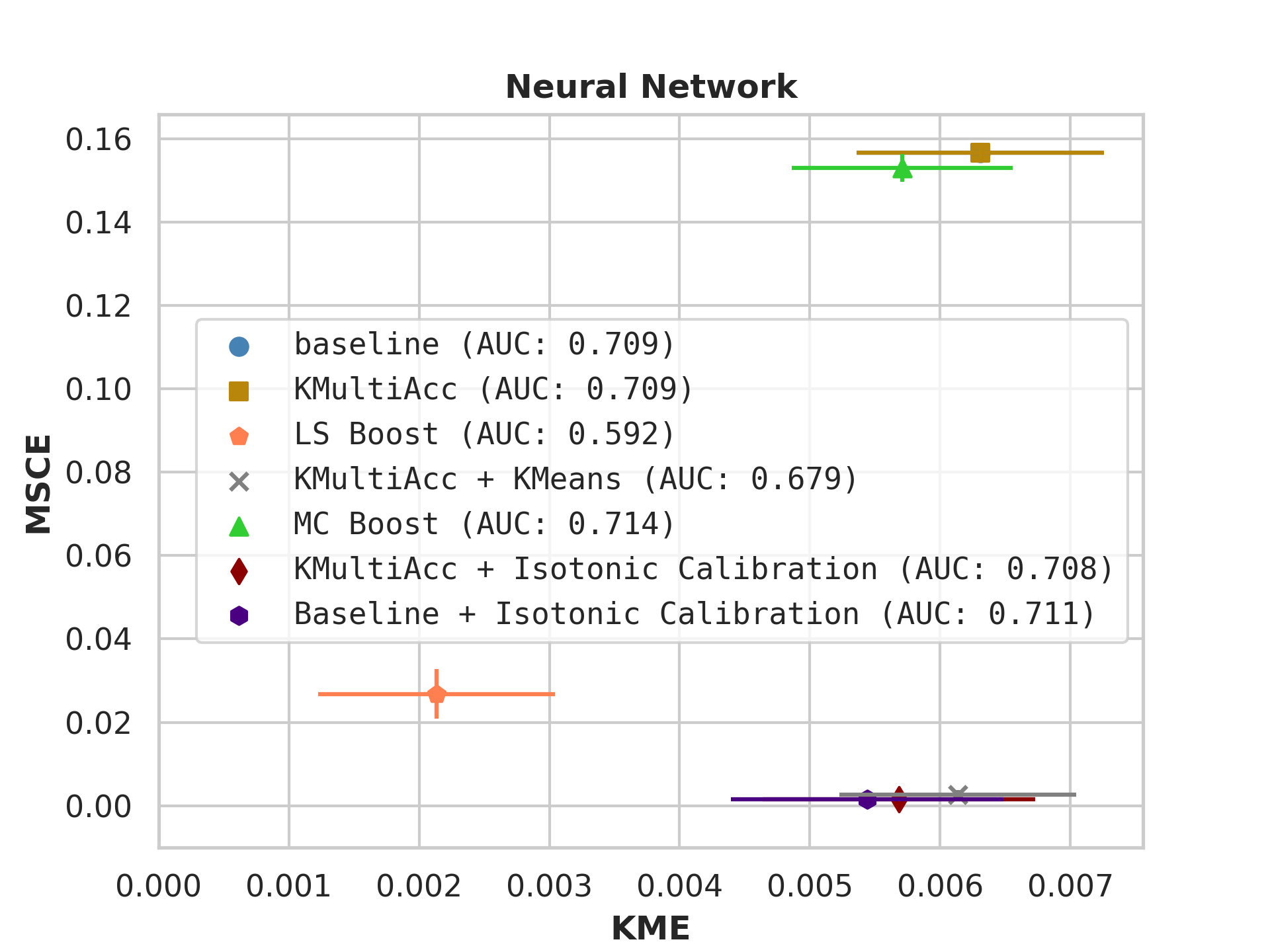
With the process described in Section 4.4, we test KMAccacross various baseline classifiers using implementations in Scikit-Learn [35]. In each US Census dataset, we execute five runs of each model on which we report, showing the mean value of each metric alongside error bars.

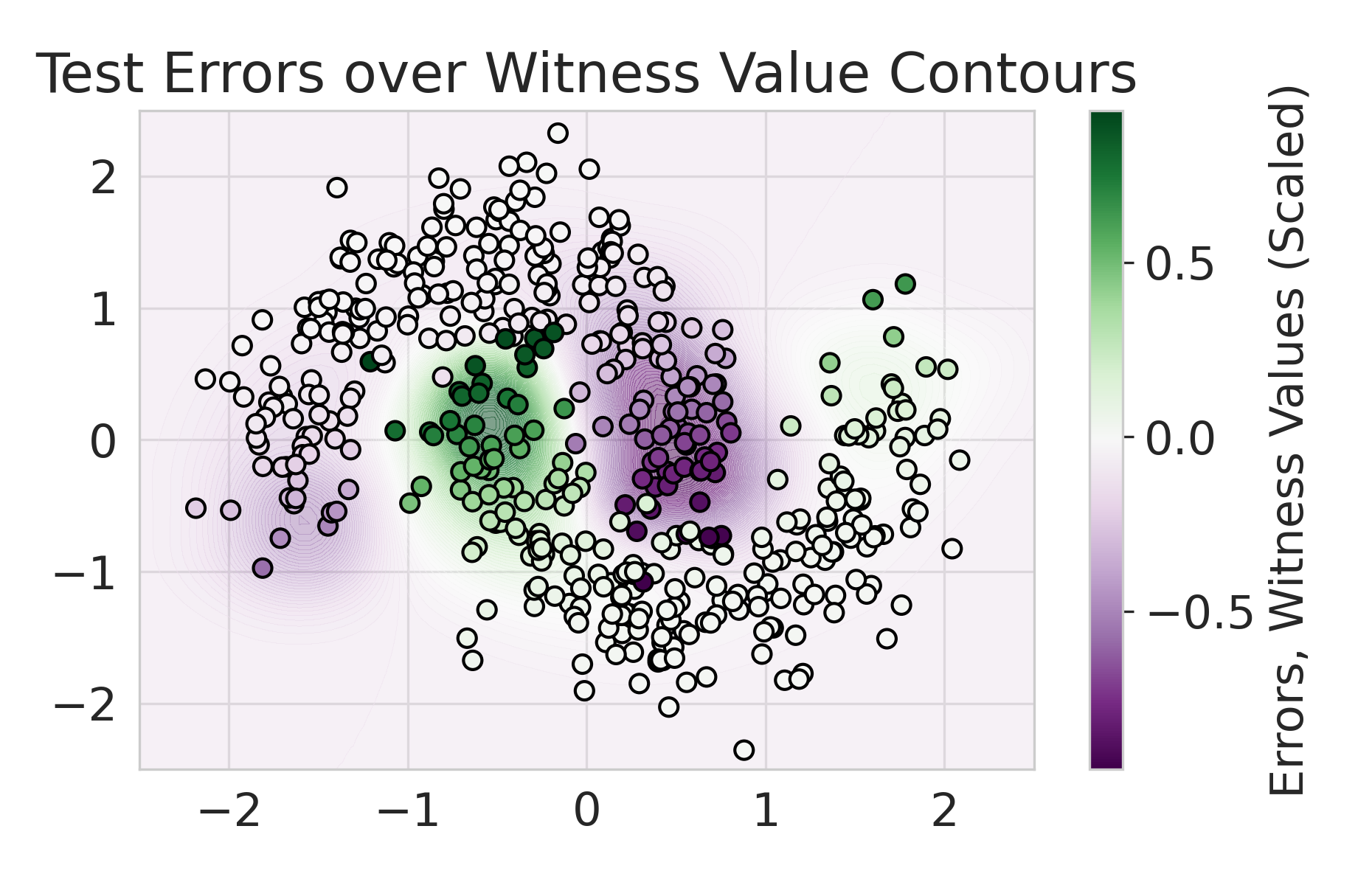
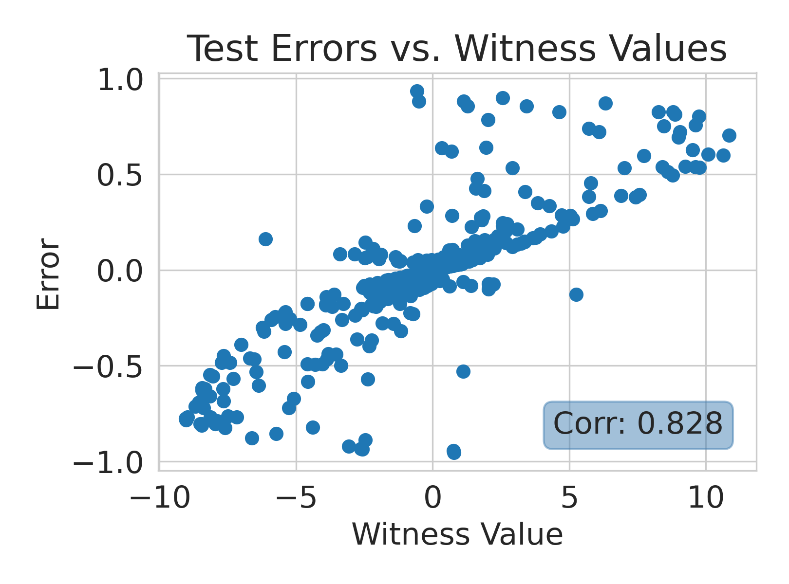
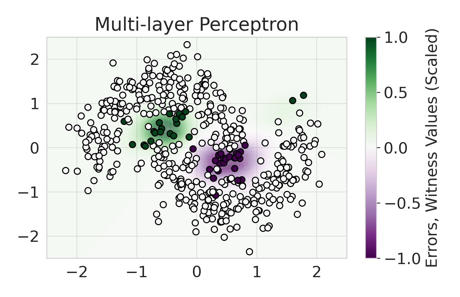
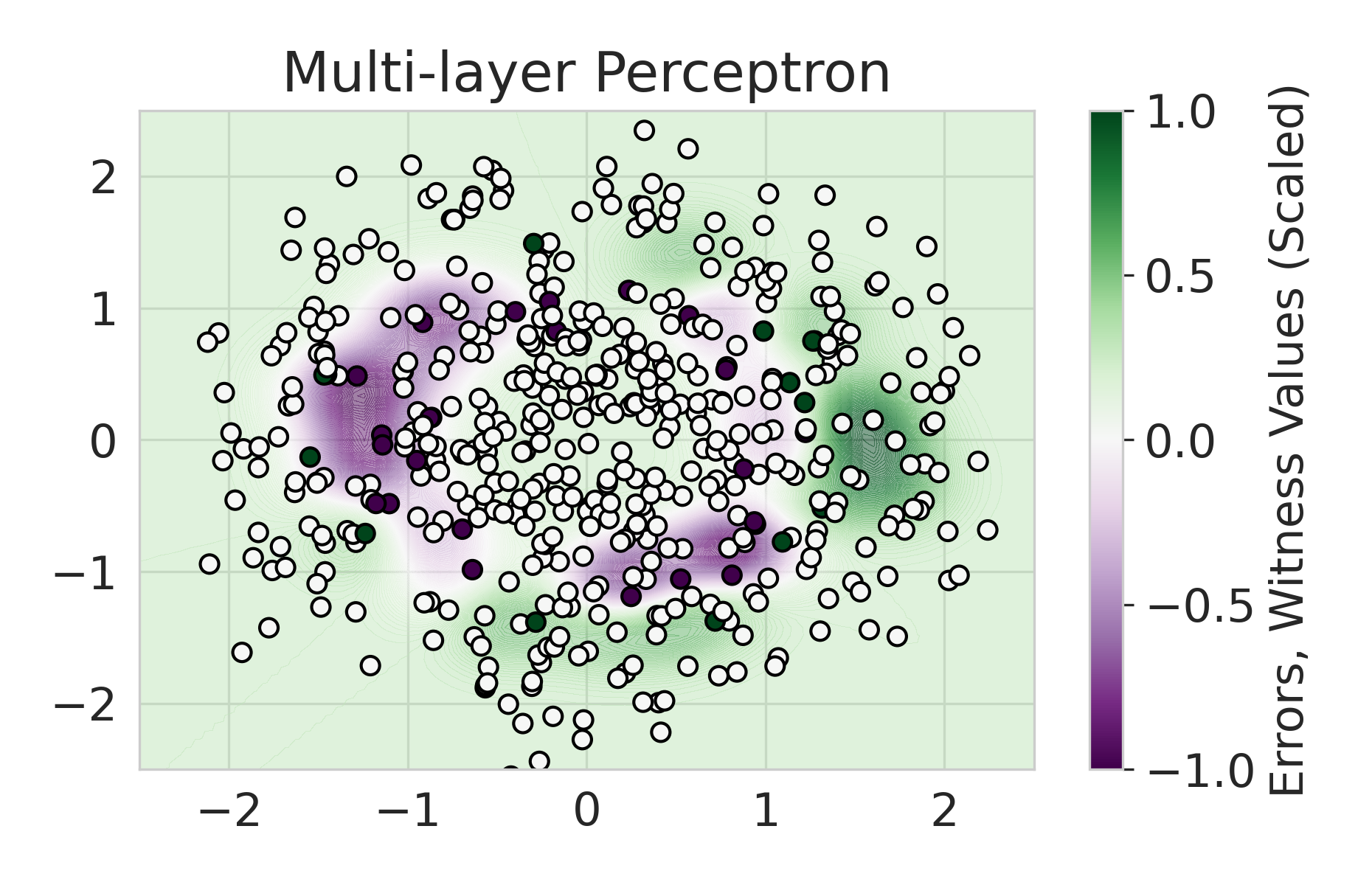
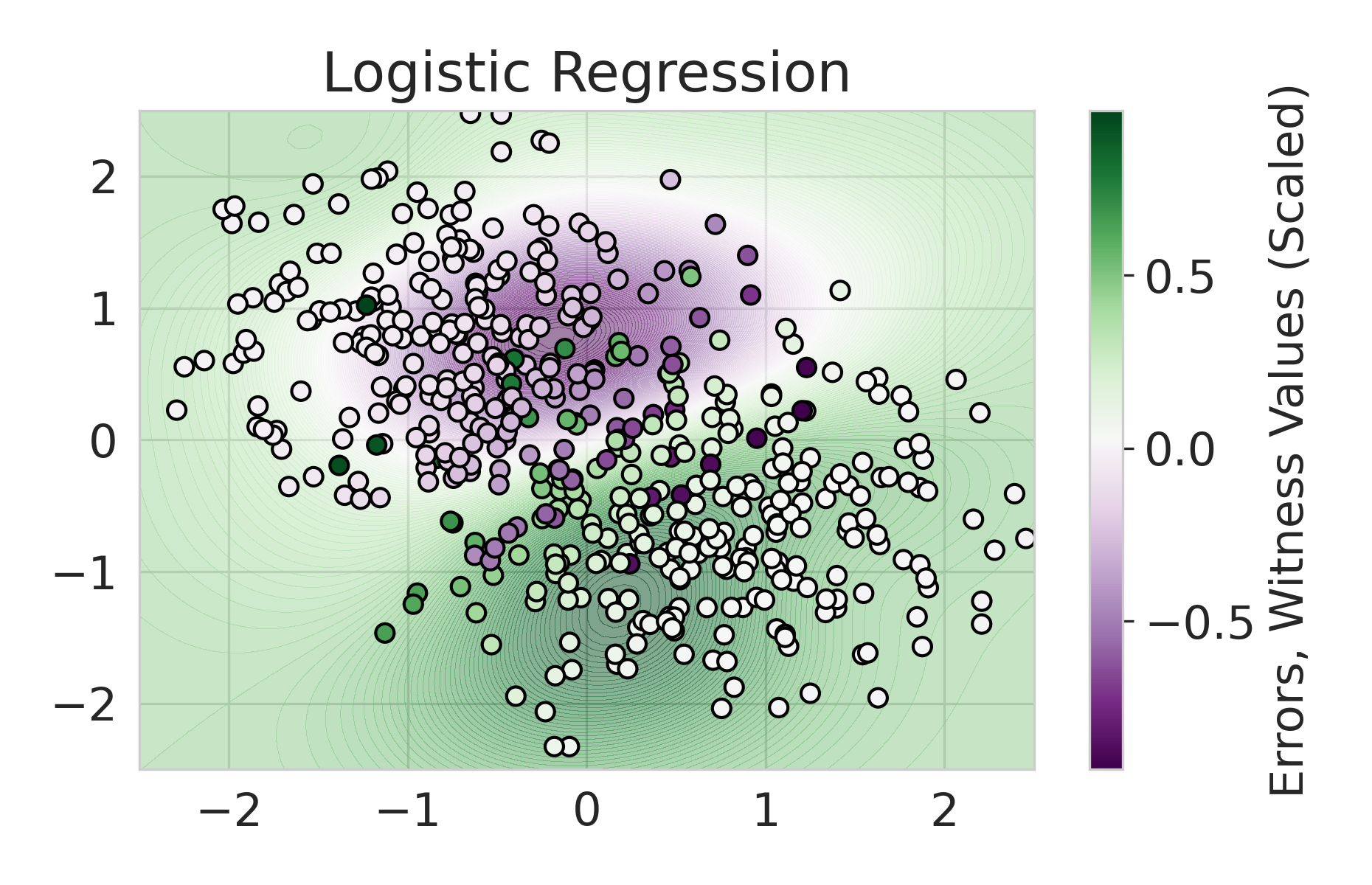
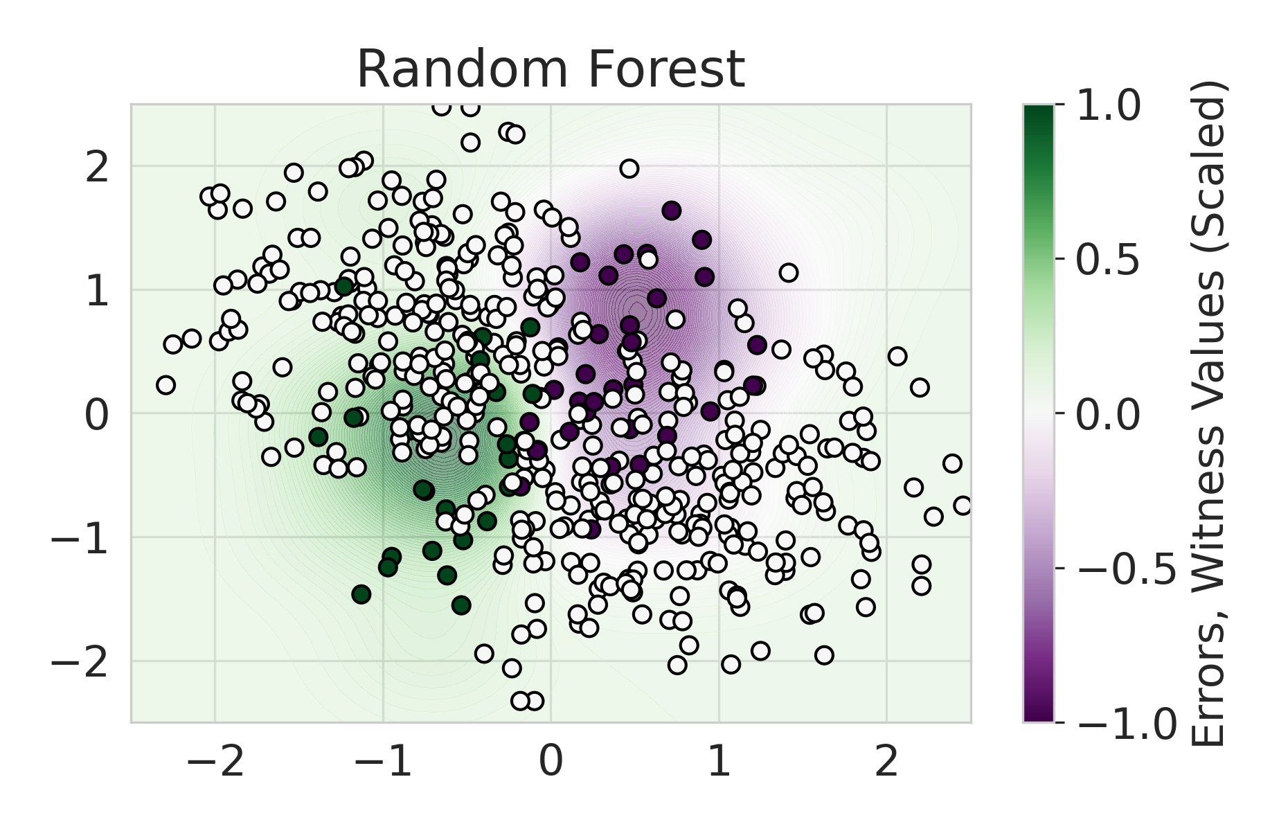
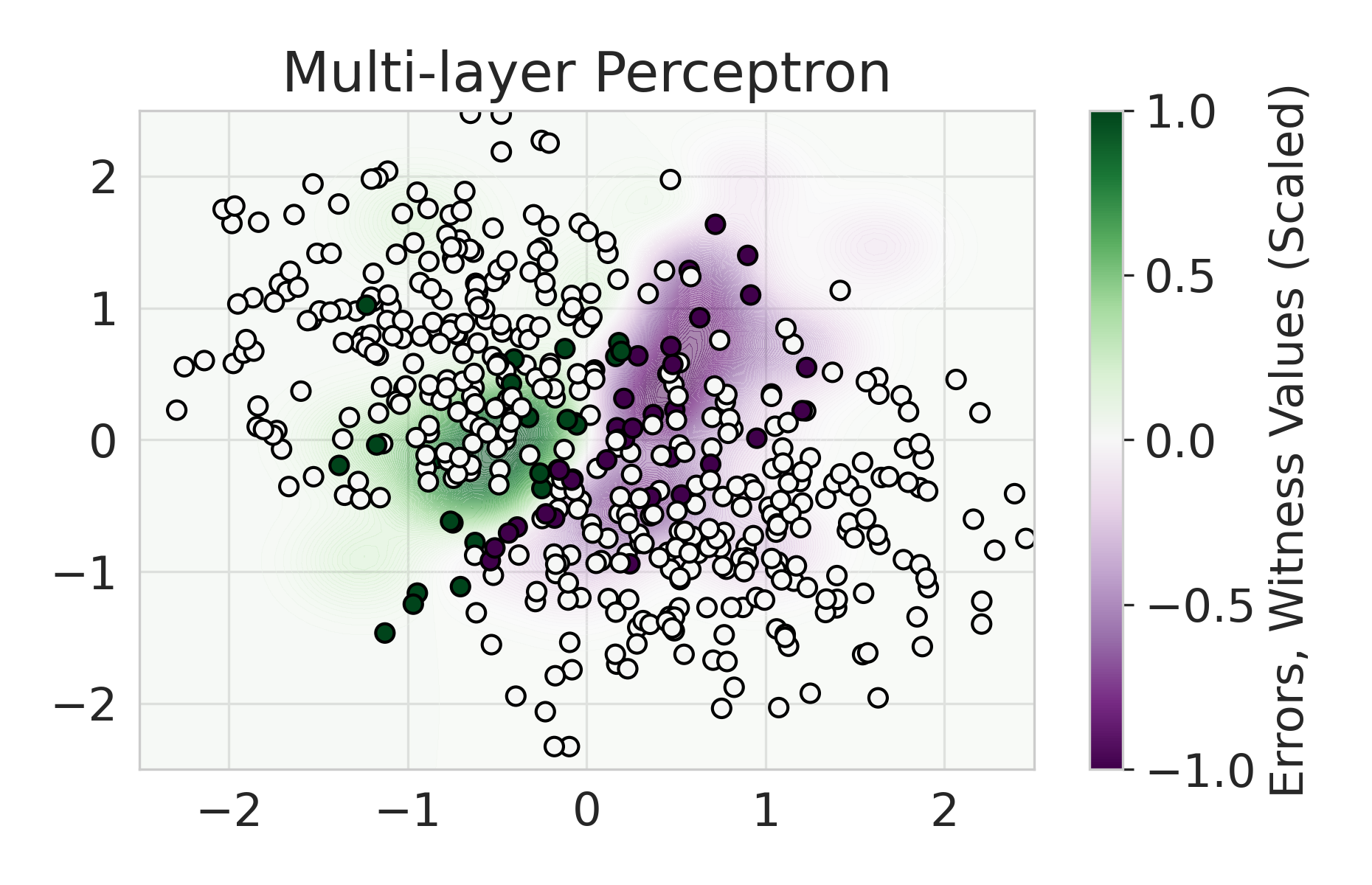
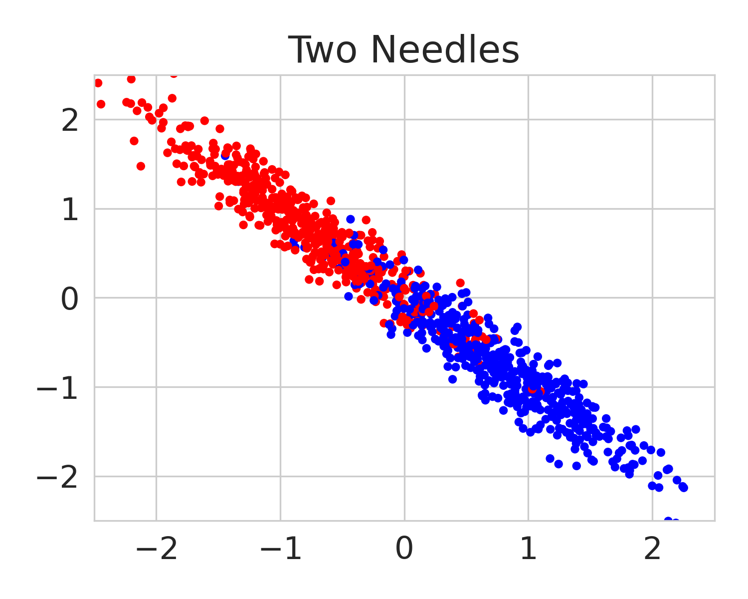
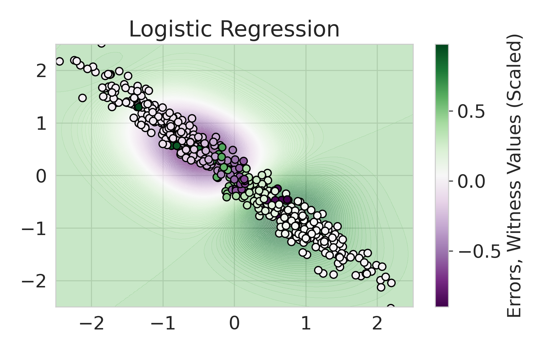
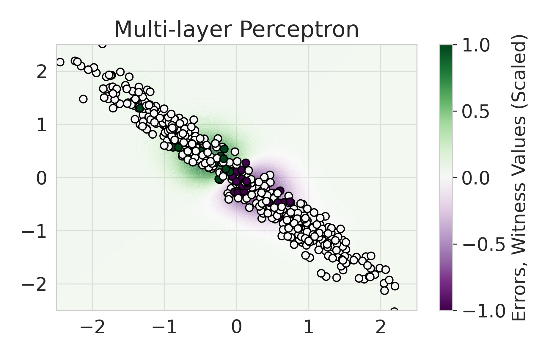
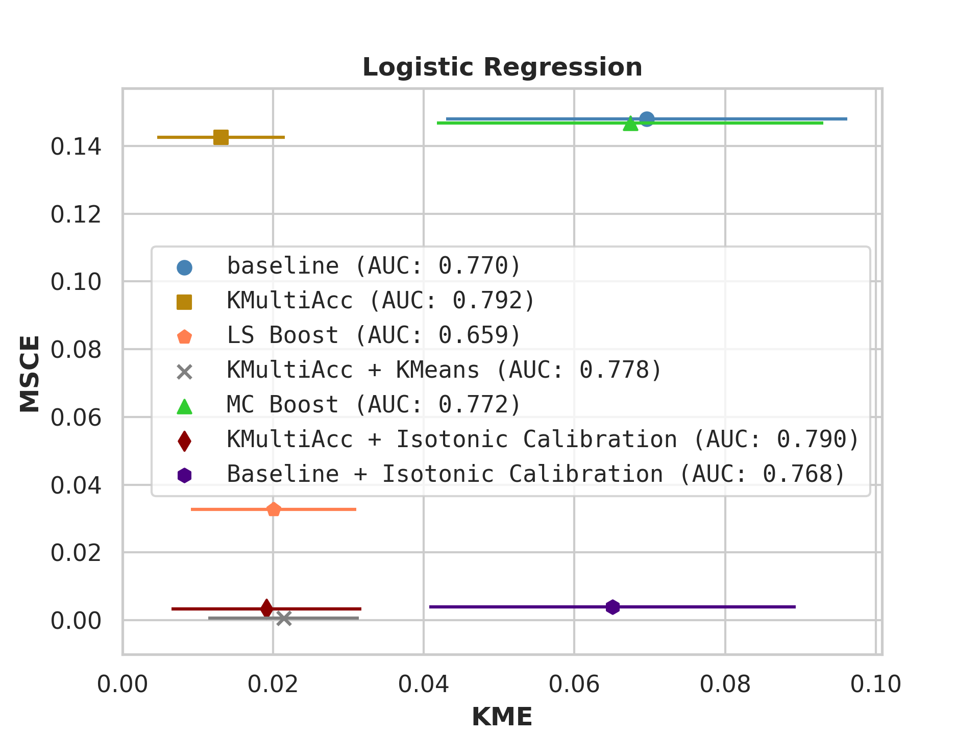
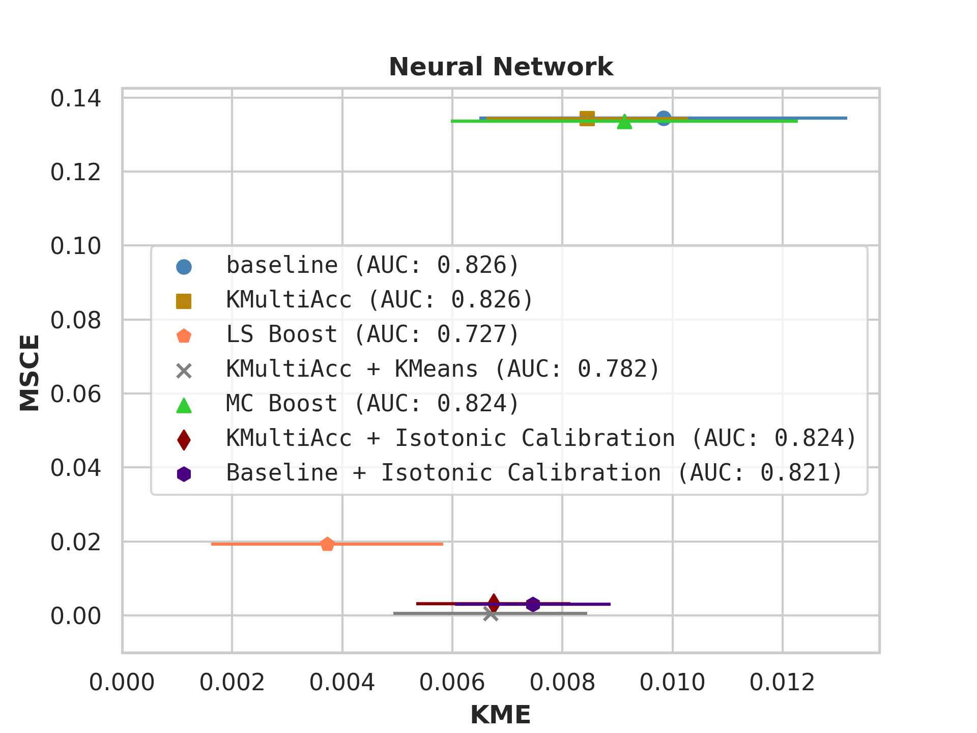
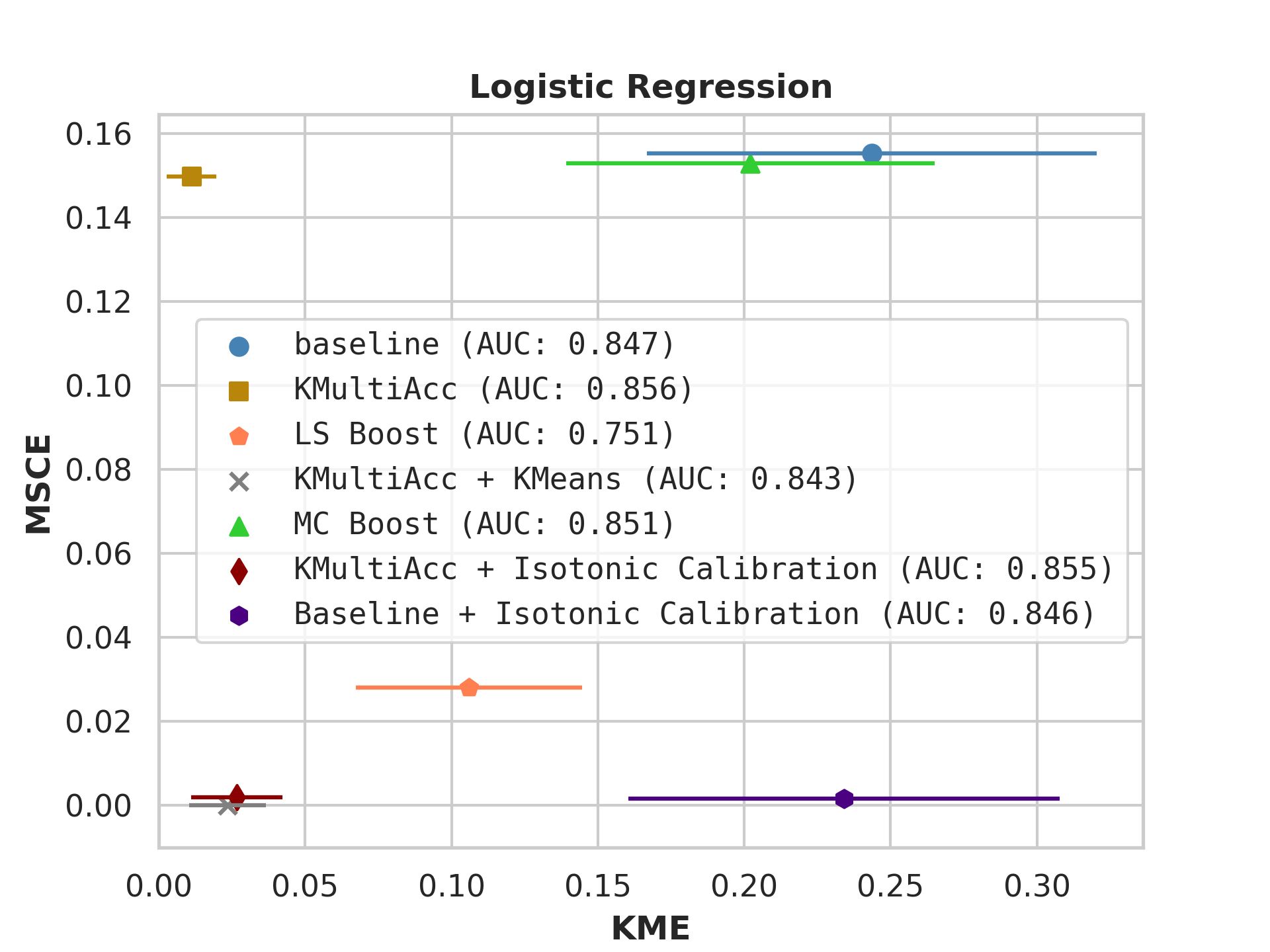
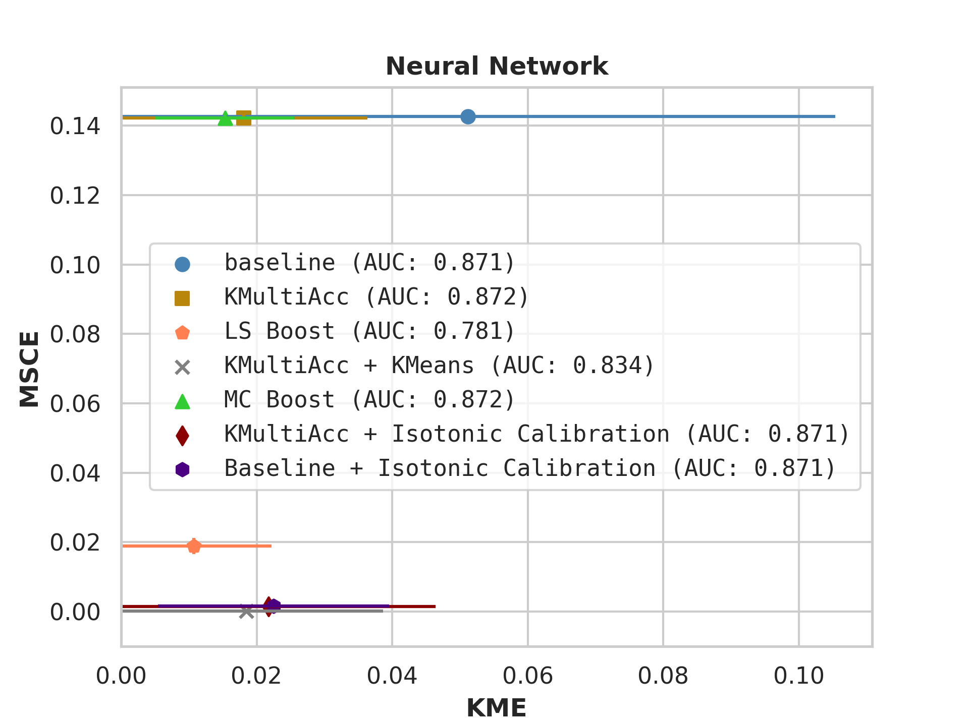
Firstly, on synthetic datasets, we demonstrate that the witness function is a good predictor of classifier error. In Figure 1, we train a logistic regression classifier on the moon and circle datasets to perform binary classification. The classifier has an accuracy of 0.85 and AUC of 0.94, and most errors occur in the middle where the red and blue classes are not linearly separable. Indeed, samples with high errors in scores $y-f(x)$ also receive high predicted errors in terms of witness function values. Indeed, the scatter plot (Right Column) illustrates the linear correlation between test error and witness value, with a high Pearson correlation coefficients of 0.828. Complete results using additional baseline models (Random Forest and Multi-layer Perceptron) are shown in Figure 3.

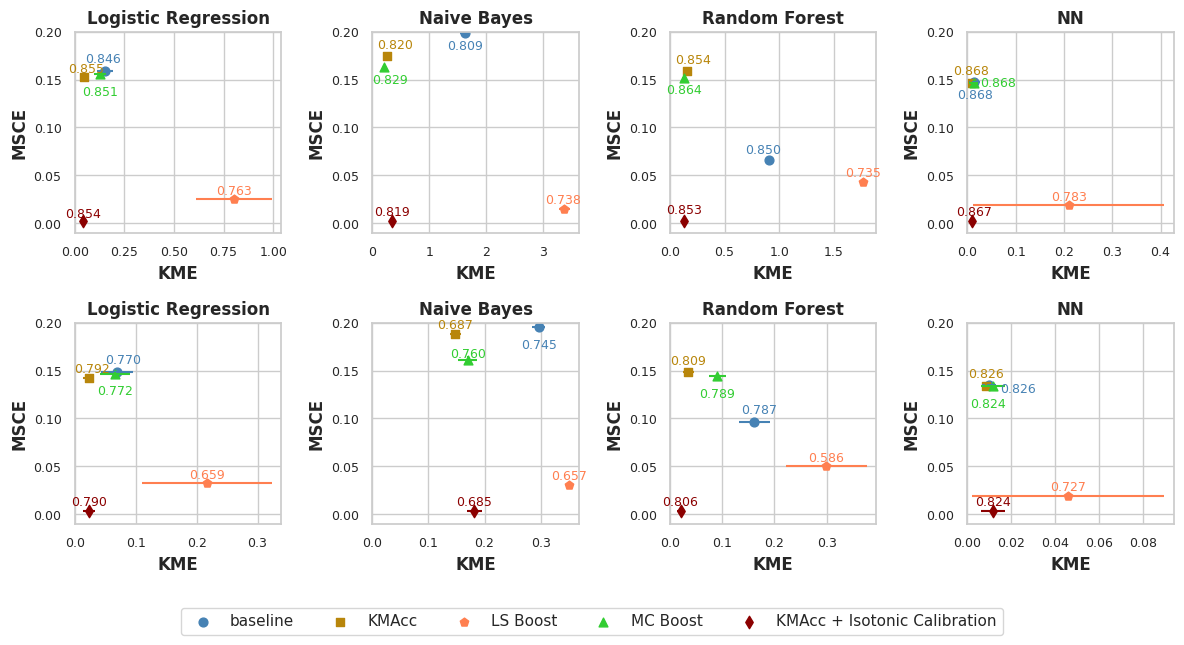
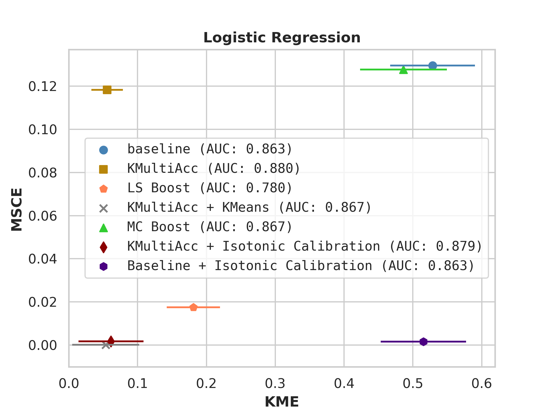
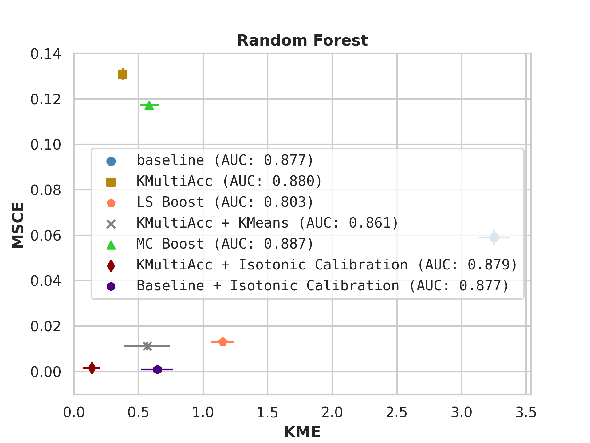
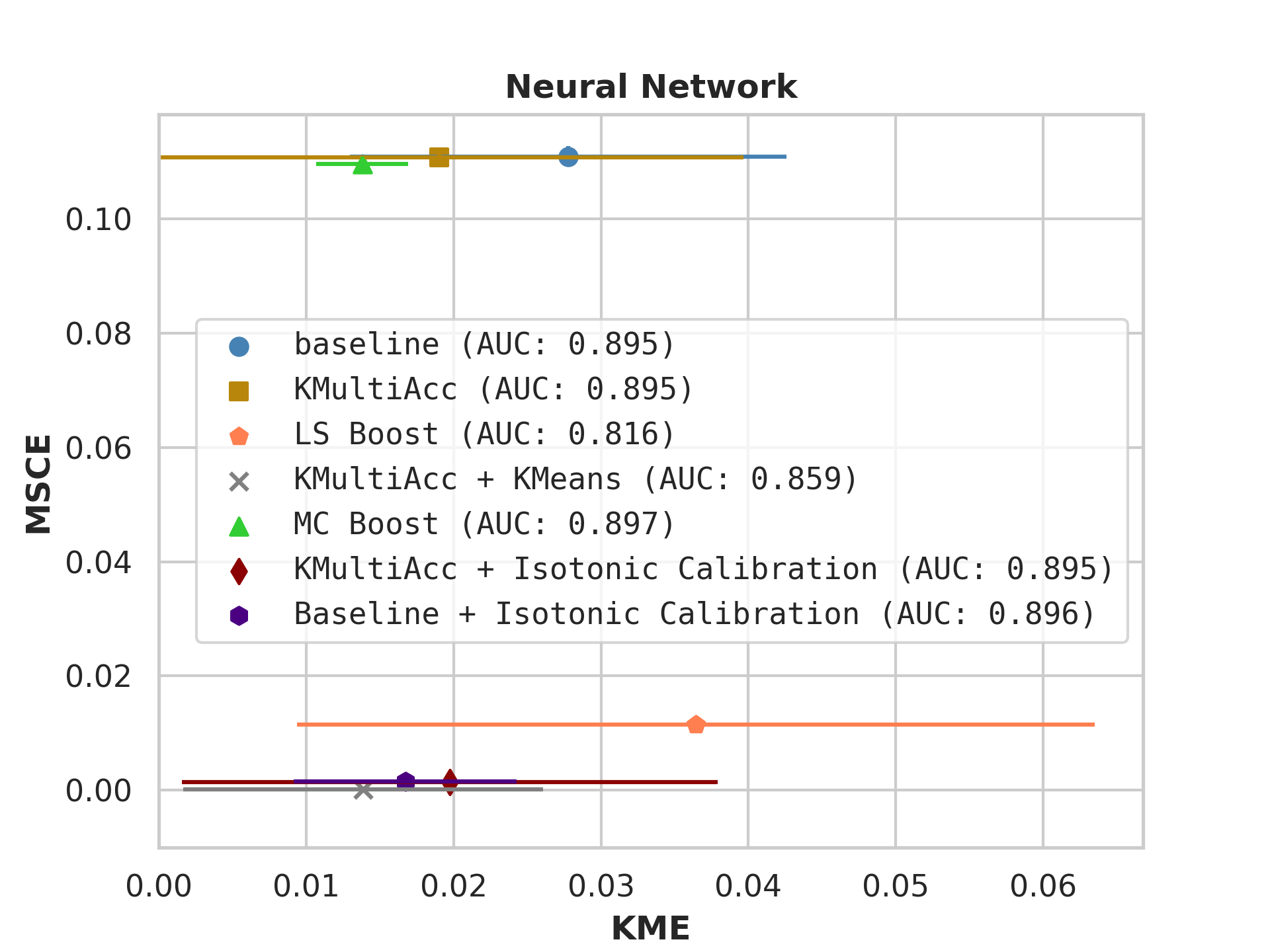
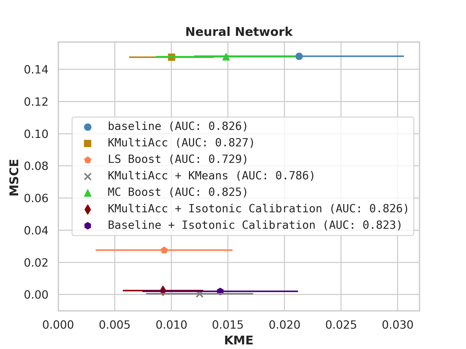
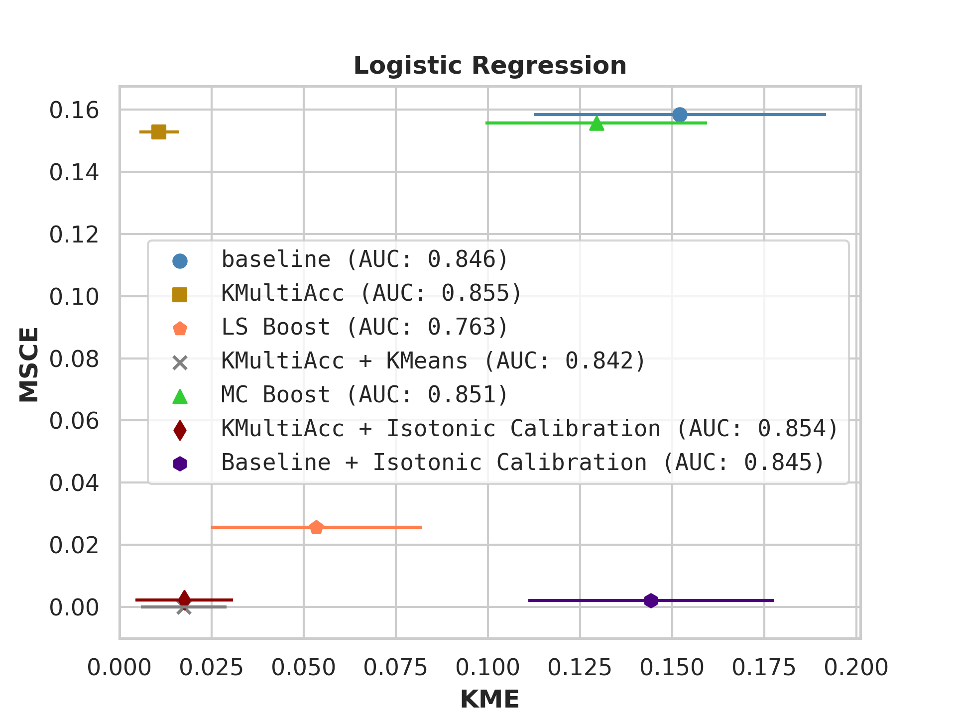
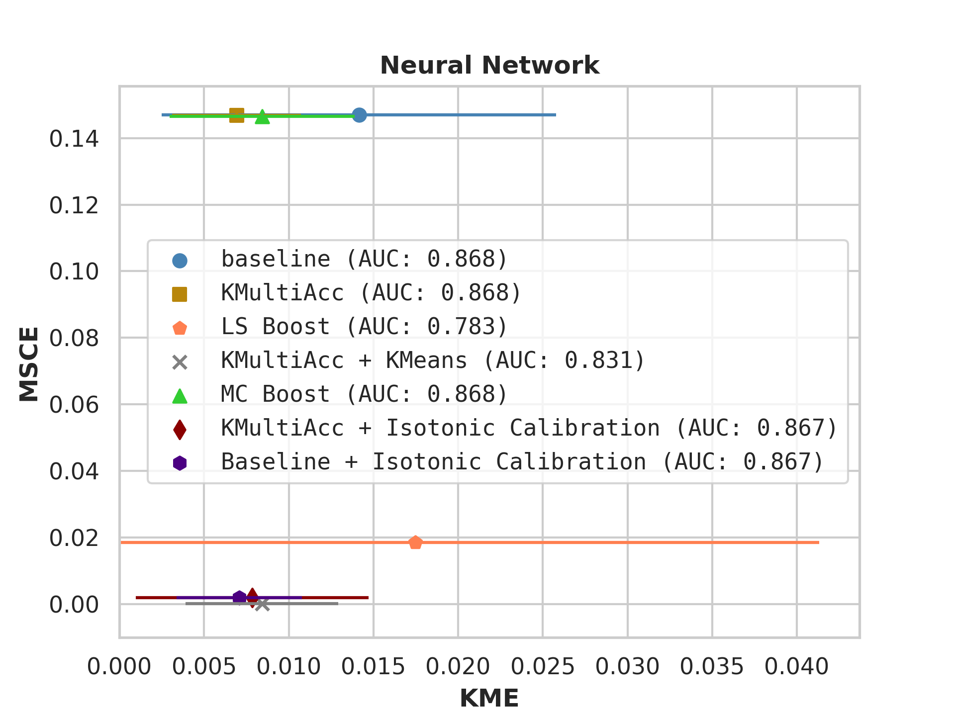
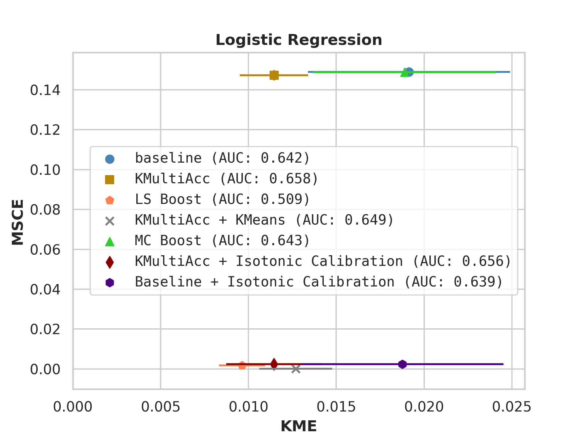
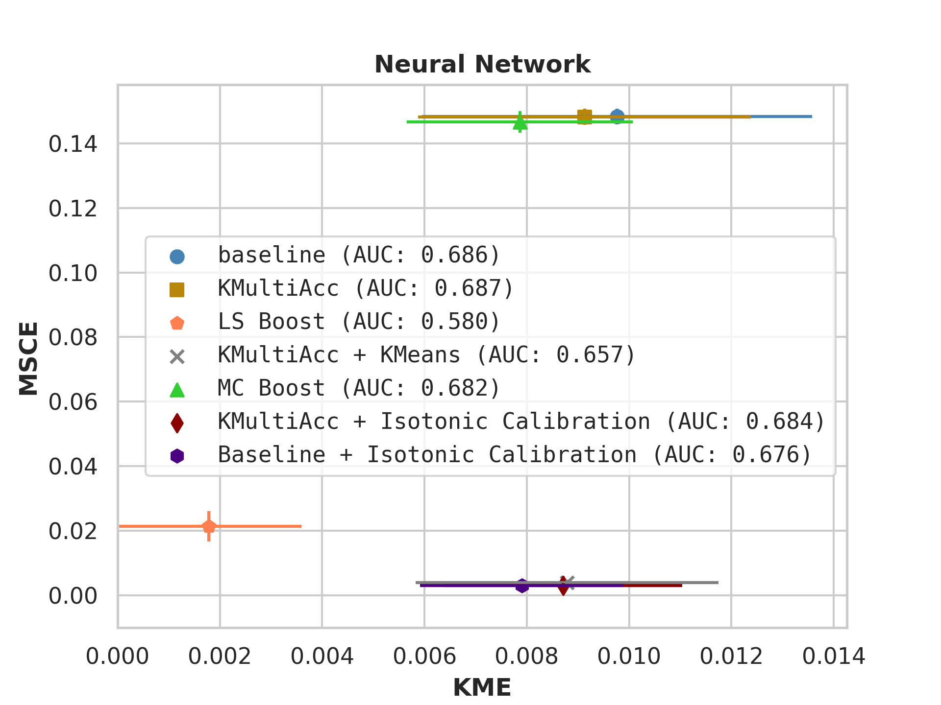
On US Census datasets and as demonstrated in Figure 10, KMAcc achieves the lowest KME relative to competing models without sacrificing AUC, and KMAcc paired with isotonic calibration achieves the lowest multi-group metrics (KME and MSCE) while maintaining competitive AUC. In Figure 10, baseline models (blue circle) have high MSCE, and most have non-negligible KME, with the exception of neural networks. Post-processing the baseline models using KMAcc (yellow rectangle), we see a significant reduction in KME from the baseline (shifting to the left of the plot), and in a majority of experiments, the post-processed models achieve, on the test set, the pre-specified KME constraint with $\gamma_{k}(g,P_{\boldsymbol{X},Y})<.01$ . To target low calibration error (measured by MSCE on the y-axis), we apply off-the-shelf isotonic calibration on top of KMAcc. We observe that applying KMAcc $+$ Isotonic Calibration (red diamond) to baseline results in low errors on both axes (KME and MSCE). Across all baselines and experiments, applying either KMAccor KMAcc $+$ Isotonic Calibration does not degrade the predictive power of the models – the AUCs (labeled next to each model) of models corrected by the proposed methods either stay relatively unchanged or improved.

Competing method MCBoost achieves effective reduction in KME with minimal improvement on MSCE, without sacrificing AUC. We note that KMAcc+Isotonic Calibration enjoys comparable or better performance with regards to MCBoost on KME and better performance on MSCE, while eliminating the need for iterative updates to minimize miscalibration that is required in MCBoost. LSBoost(orange polygon) achieves low MSCE while worsening both KME and AUC.

5 Discussion and Conclusion

We connect the multi-group notions to Integral Probability Measures (IPM), providing a unifying statistical perspective on Multiaccuracy, Multicalibration, and OI. This perspective leads us to a simple yet powerful algorithm (KMAcc) for achieving multiaccuracy with respect to a class of functions defined by an RKHS. KMAcc boils down to first predicting the error of the classifier using the witness function, and then subtracting the error away. This algorithm enjoys provable performance guarantees and empirically achieves favorable accuracy and multi-group metrics relative to competing methods.

A limitation of our empirical analysis in comparison to other methods is that we optimize over the calibration function class being the unit-ball RKHS with the RBF kernel, which may not be the set of calibration functions for which other benchmarks achieve the lowest multiaccuracy or multicalibration error on. Furthermore, while the proposed method achieves favorable multicalibration results, this algorithm does not have provable guarantees for multicalibration. Developing a multicalibration-ensuring algorithm through the IPM perspective is an exciting future direction.

To conclude, this work contributes to the greater effort of reducing embedded human bias in ML fairness. To this end, we adopt RKHS as the expressive group-denoting function class to ensure multi-group notions on, rather than using predefined groups. It remains an open question to explore the structure of the witness function – the most biased group-denoting function in the RKHS – and its relationship to the predefined group attributes, which may inform us of the intersectionality and the structure of errors in ML models.

References

[1] Alekh Agarwal, Alina Beygelzimer, Miroslav Dudík, John Langford, and Hanna Wallach. A reductions approach to fair classification. In International conference on machine learning, pages 60–69. PMLR, 2018. URL: http://proceedings.mlr.press/v80/agarwal18a.html.
[2] Wael Alghamdi, Hsiang Hsu, Haewon Jeong, Hao Wang, Peter Michalak, Shahab Asoodeh, and Flavio Calmon. Beyond adult and compas: Fair multi-class prediction via information projection. Advances in Neural Information Processing Systems, 35:38747–38760, 2022.
[3] Solon Barocas, Moritz Hardt, and Arvind Narayanan. Fairness and machine learning: Limitations and opportunities. MIT Press, 2023.
[4] Alain Berlinet and Christine Thomas-Agnan. Reproducing Kernel Hilbert Spaces in Probability and Statistics. Springer, 1 edition, 2004. doi:10.1007/9781441990969.
[5] Stephen P Boyd and Lieven Vandenberghe. Convex optimization. Cambridge university press, 2004.
[6] Peng Cui, Wenbo Hu, and Jun Zhu. Calibrated reliable regression using maximum mean discrepancy. In H. Larochelle, M. Ranzato, R. Hadsell, M.F. Balcan, and H. Lin, editors, Advances in Neural Information Processing Systems, volume 33, pages 17164–17175. Curran Associates, Inc., 2020. URL: https://proceedings.neurips.cc/paper_files/paper/2020/file/c74c4bf0dad9cbae3d80faa054b7d8ca-Paper.pdf.
[7] A Philip Dawid. The well-calibrated bayesian. Journal of the American Statistical Association, 77(379):605–610, 1982.
[8] Zhun Deng, Cynthia Dwork, and Linjun Zhang. Happymap: A generalized multi-calibration method. arXiv preprint arXiv:2303.04379, 2023. doi:10.48550/arXiv.2303.04379.
[9] Cynthia Dwork, Michael P Kim, Omer Reingold, Guy N Rothblum, and Gal Yona. Outcome indistinguishability. In Proceedings of the 53rd Annual ACM SIGACT Symposium on Theory of Computing, pages 1095–1108, 2021. doi:10.1145/3406325.3451064.
[10] Cynthia Dwork, Daniel Lee, Huijia Lin, and Pranay Tankala. From pseudorandomness to multi-group fairness and back. In The Thirty Sixth Annual Conference on Learning Theory, pages 3566–3614. PMLR, 2023. URL: https://proceedings.mlr.press/v195/dwork23a.html.
[11] Vitaly Feldman. Distribution-specific agnostic boosting. In International Conference on Supercomputing, 2009. URL: https://api.semanticscholar.org/CorpusID:2787595.
[12] Sorelle A Friedler, Carlos Scheidegger, Suresh Venkatasubramanian, Sonam Choudhary, Evan P Hamilton, and Derek Roth. A comparative study of fairness-enhancing interventions in machine learning. In Proceedings of the conference on fairness, accountability, and transparency, pages 329–338, 2019. doi:10.1145/3287560.3287589.
[13] Sumegha Garg, Christopher Jung, Omer Reingold, and Aaron Roth. Oracle efficient online multicalibration and omniprediction. In Proceedings of the 2024 Annual ACM-SIAM Symposium on Discrete Algorithms (SODA), pages 2725–2792. SIAM, 2024. doi:10.1137/1.9781611977912.98.
[14] Ira Globus-Harris, Varun Gupta, Christopher Jung, Michael Kearns, Jamie Morgenstern, and Aaron Roth. Multicalibrated regression for downstream fairness. arXiv preprint arXiv:2209.07312, 2022. doi:10.48550/arXiv.2209.07312.
[15] Ira Globus-Harris, Declan Harrison, Michael Kearns, Aaron Roth, and Jessica Sorrell. Multicalibration as boosting for regression. arXiv preprint arXiv:2301.13767, 2023. doi:10.48550/arXiv.2301.13767.
[16] Robert Kent Goodrich. A riesz representation theorem. In Proc. Amer. Math. Soc, volume 24, pages 629–636, 1970.
[17] Parikshit Gopalan, Lunjia Hu, Michael P Kim, Omer Reingold, and Udi Wieder. Loss minimization through the lens of outcome indistinguishability. arXiv preprint arXiv:2210.08649, 2022. doi:10.48550/arXiv.2210.08649.
[18] Parikshit Gopalan, Adam Tauman Kalai, Omer Reingold, Vatsal Sharan, and Udi Wieder. Omnipredictors. arXiv preprint arXiv:2109.05389, 2021. arXiv:2109.05389.
[19] Arthur Gretton, Karsten Borgwardt, Malte Rasch, Bernhard Schölkopf, and Alex Smola. A kernel method for the two-sample-problem. Advances in neural information processing systems, 19, 2006.
[20] Nika Haghtalab, Michael Jordan, and Eric Zhao. A unifying perspective on multi-calibration: Game dynamics for multi-objective learning. Advances in Neural Information Processing Systems, 36, 2024.
[21] Moritz Hardt, Eric Price, and Nati Srebro. Equality of opportunity in supervised learning. Advances in neural information processing systems, 29, 2016.
[22] Ursula Hébert-Johnson, Michael Kim, Omer Reingold, and Guy Rothblum. Multicalibration: Calibration for the (computationally-identifiable) masses. In International Conference on Machine Learning, pages 1939–1948. PMLR, 2018.
[23] Emmie Hine and Luciano Floridi. The blueprint for an ai bill of rights: in search of enaction, at risk of inaction. Minds and Machines, pages 1–8, 2023.
[24] Max Hort, Zhenpeng Chen, Jie M Zhang, Federica Sarro, and Mark Harman. Bia mitigation for machine learning classifiers: A comprehensive survey. arXiv preprint arXiv:2207.07068, 2022. doi:10.48550/arXiv.2207.07068.
[25] Faisal Kamiran, Asim Karim, and Xiangliang Zhang. Decision theory for discrimination-aware classification. In 2012 IEEE 12th international conference on data mining, pages 924–929. IEEE, 2012. doi:10.1109/ICDM.2012.45.
[26] Michael Kearns, Seth Neel, Aaron Roth, and Zhiwei Steven Wu. Preventing fairness gerrymandering: Auditing and learning for subgroup fairness. In International conference on machine learning, pages 2564–2572. PMLR, 2018.
[27] Been Kim, Rajiv Khanna, and Oluwasanmi O Koyejo. Examples are not enough, learn to criticize! criticism for interpretability. Advances in neural information processing systems, 29, 2016.
[28] Michael P Kim, Amirata Ghorbani, and James Zou. Multiaccuracy: Black-box post-processing for fairness in classification. In Proceedings of the 2019 AAAI/ACM Conference on AI, Ethics, and Society, pages 247–254, 2019. doi:10.1145/3306618.3314287.
[29] Michael P. Kim, Christoph Kern, Shafi Goldwasser, and Frauke Krueter. Universal adaptability: Target-independent inference that competes with propensity scoring. Proceedings of the National Academy of Sciences, page 119(4):e2108097119, 2022.
[30] Aviral Kumar, Sunita Sarawagi, and Ujjwal Jain. Trainable calibration measures for neural networks from kernel mean embeddings. In International Conference on Machine Learning, pages 2805–2814. PMLR, 2018.
[31] Carol Xuan Long, Hsiang Hsu, Wael Alghamdi, and Flavio Calmon. Individual arbitrariness and group fairness. In Thirty-seventh Conference on Neural Information Processing Systems, 2023.
[32] Charles Marx, Sofian Zalouk, and Stefano Ermon. Calibration by distribution matching: Trainable kernel calibration metrics. arXiv preprint arXiv:2310.20211, 2023. doi:10.48550/arXiv.2310.20211.
[33] Alfred Müller. Integral probability metrics and their generating classes of functions. Advances in applied probability, 29(2):429–443, 1997.
[34] Alexandru Niculescu-Mizil and Rich Caruana. Predicting good probabilities with supervised learning. In Proceedings of the 22nd international conference on Machine learning, pages 625–632, 2005. doi:10.1145/1102351.1102430.
[35] F. Pedregosa, G. Varoquaux, A. Gramfort, V. Michel, B. Thirion, O. Grisel, M. Blondel, P. Prettenhofer, R. Weiss, V. Dubourg, J. Vanderplas, A. Passos, D. Cournapeau, M. Brucher, M. Perrot, and E. Duchesnay. Scikit-learn: Machine learning in Python. Journal of Machine Learning Research, 12:2825–2830, 2011. doi:10.5555/1953048.2078195.
[36] Hao Song, Tom Diethe, Meelis Kull, and Peter Flach. Distribution calibration for regression. In International Conference on Machine Learning, pages 5897–5906. PMLR, 2019. URL: http://proceedings.mlr.press/v97/song19a.html.
[37] Bharath K Sriperumbudur, Kenji Fukumizu, Arthur Gretton, Bernhard Schölkopf, and Gert RG Lanckriet. On the empirical estimation of integral probability metrics, 2012.
[38] Bharath K Sriperumbudur, Kenji Fukumizu, and Gert RG Lanckriet. Universality, characteristic kernels and rkhs embedding of measures. Journal of Machine Learning Research, 12(7), 2011.
[39] David Widmann, Fredrik Lindsten, and Dave Zachariah. Calibration tests in multi-class classification: A unifying framework. Advances in neural information processing systems, 32, 2019.
[40] David Widmann, Fredrik Lindsten, and Dave Zachariah. Calibration tests beyond classification. arXiv preprint arXiv:2210.13355, 2022. doi:10.48550/arXiv.2210.13355.
[41] Lujing Zhang, Aaron Roth, and Linjun Zhang. Fair risk control: A generalized framework for calibrating multi-group fairness risks. arXiv preprint arXiv:2405.02225, 2024. doi:10.48550/arXiv.2405.02225.

Appendix

Appendix A Details of Theoretical Framework

From Equation (37), we show that it is a quadratic program (QP). To begin, writing $\mathcal{D}=\{(\boldsymbol{x}_{j},y_{j})\}_{j=1}^{n}$ and denoting

\boldsymbol{f}_{\mathcal{D}}=(f(\boldsymbol{x}_{1}),\cdots,f(\boldsymbol{x}_{n% }))^{T},\boldsymbol{g}=(g(\boldsymbol{x}_{1}),\cdots,g(\boldsymbol{x}_{n}))^{T},

(41)

the objective function becomes the quadratic function $\frac{1}{2}\|\boldsymbol{f}_{\mathcal{D}}-\boldsymbol{g}\|_{2}^{2}$ . Similarly, the constraint is a linear inequality in $\boldsymbol{g}$ , which we write as $\boldsymbol{A}_{\mathcal{D}_{0},\mathcal{D}}\ \boldsymbol{g}\leq\boldsymbol{b}% _{\mathcal{D}_{0},\mathcal{D}}$ , where $\boldsymbol{A}_{\mathcal{D}_{0},\mathcal{D}}\in\mathbb{R}^{(2n+2)\times n}$ and $\boldsymbol{b}_{{\mathcal{D}_{0},\mathcal{D}}}\in\mathbb{R}^{2n+2}$ are fixed and determined by $\mathcal{D}_{0}$ and $\mathcal{D}$ in view of equation (33) for the empirical witness function $c_{k,\mathcal{D}_{0},f}^{\star}$ . Explicitly, denoting $\mathcal{D}_{0}=\{(\widetilde{\boldsymbol{x}}_{i},\widetilde{y}_{i})\}_{i=1}^{m}$ , let us use the shorthands

\boldsymbol{y}_{\mathcal{D}}=(y_{1},\cdots,y_{n})^{T},\boldsymbol{c}_{\mathcal% {D}_{0},\mathcal{D}}=(c_{k,\mathcal{D}_{0},f}^{\star}(\boldsymbol{x}_{1}),% \cdots,c_{k,\mathcal{D}_{0},f}^{\star}(\boldsymbol{x}_{n}))^{T}.

(42)

Then, the multiaccuracy constraint in (37) can be written as $|\boldsymbol{c}_{\mathcal{D}_{0},\mathcal{D}}^{T}\boldsymbol{g}/n-\boldsymbol{% c}_{\mathcal{D}_{0},\mathcal{D}}^{T}\boldsymbol{y}_{\mathcal{D}}/n|\leq\alpha$ . Taking the search space into consideration (i.e., $g$ evaluates to $[0,1]$ ), we see that (37) may be rewritten as the the following QP:

	$\displaystyle\underset{\boldsymbol{g}\in\mathbb{R}^{n}}{\text{minimize}}$	$\displaystyle\quad\frac{1}{2}\left\\|\boldsymbol{f}_{\mathcal{D}}-\boldsymbol{g% }\right\\|_{2}^{2}$		(43)
	subject to	$\displaystyle\quad\boldsymbol{A}_{\mathcal{D}_{0},\mathcal{D}}\ \boldsymbol{g}% \leq\boldsymbol{b}_{\mathcal{D}_{0},\mathcal{D}},$

where we define the constraint’s matrix and vector by

\boldsymbol{A}_{\mathcal{D}_{0},\mathcal{D}}\coloneqq\begin{pmatrix}% \boldsymbol{c}_{\mathcal{D}_{0},\mathcal{D}}^{T}/n\\ -\boldsymbol{c}_{\mathcal{D}_{0},\mathcal{D}}^{T}/n\\ \boldsymbol{I}_{n}\\ -\boldsymbol{I}_{n}\end{pmatrix},\boldsymbol{b}_{\mathcal{D}_{0},\mathcal{D}}% \coloneqq\begin{pmatrix}\alpha+\boldsymbol{c}_{\mathcal{D}_{0},\mathcal{D}}^{T% }\boldsymbol{y}/n\\ \alpha-\boldsymbol{c}_{\mathcal{D}_{0},\mathcal{D}}^{T}\boldsymbol{y}/n\\ \boldsymbol{1}_{n}\\ \boldsymbol{0}_{n}\end{pmatrix}.

(44)

Note that the witness function for a kernel $k:\mathcal{X}^{2}\to\mathbb{R}$ , dataset $\mathcal{D}_{0}=\{(\widetilde{\boldsymbol{x}}_{j},\widetilde{y}_{j})\}_{j\in[m]}$ , and predictor $g:\mathcal{X}\to[0,1]$ is given by

c_{k,\mathcal{D}_{0},g}^{\star}(\boldsymbol{x})=\frac{\theta_{k,\mathcal{D}_{0% },g}}{m}(\widetilde{\boldsymbol{g}}-\widetilde{\boldsymbol{y}})^{T}\widetilde{% \boldsymbol{k}}(\boldsymbol{x}),

(45)

c_{k,\mathcal{D}_{0},g}^{\star}(\boldsymbol{x})=\frac{(\widetilde{\boldsymbol{% g}}-\widetilde{\boldsymbol{y}})^{T}\widetilde{\boldsymbol{k}}(\boldsymbol{x})}% {\sqrt{(\widetilde{\boldsymbol{g}}-\widetilde{\boldsymbol{y}})^{T}\widetilde{% \boldsymbol{K}}(\widetilde{\boldsymbol{g}}-\widetilde{\boldsymbol{y}})}}

(46)

where $\widetilde{\boldsymbol{k}}:\mathcal{X}\to\mathbb{R}^{m}$ is the vector-valued function defined by $\widetilde{\boldsymbol{k}}(\boldsymbol{x})\coloneqq(k(\boldsymbol{x},% \widetilde{\boldsymbol{x}}_{j}))_{j\in[m]}$ , $\widetilde{\boldsymbol{g}}\coloneqq(g(\widetilde{\boldsymbol{x}}_{j}))_{j\in[m]}$ and $\widetilde{\boldsymbol{y}}\coloneqq(\widetilde{y}_{j})_{j\in[m]}$ are fixed vectors, and $\theta_{k,\mathcal{D}_{0},g}$ is a normalizing constant that is unique up to sign. We may compute $\theta_{k,\mathcal{D}_{0},g}$ by setting $\|c_{k,\mathcal{D}_{0},g}^{\star}\|_{\mathcal{H}_{k}}=1$ , namely, we have

\theta_{k,\mathcal{D}_{0},g}^{2}=\frac{m^{2}}{(\widetilde{\boldsymbol{g}}-% \widetilde{\boldsymbol{y}})^{T}\widetilde{\boldsymbol{K}}(\widetilde{% \boldsymbol{g}}-\widetilde{\boldsymbol{y}})},

(47)

where $\widetilde{\boldsymbol{K}}\coloneqq(k(\widetilde{\boldsymbol{x}}_{i},% \widetilde{\boldsymbol{x}}_{j}))_{i,j\in[m]}$ is a fixed matrix. Thus, the multiaccuracy constraint becomes

\left|\overline{\boldsymbol{h}}^{T}\overline{\boldsymbol{K}}\widetilde{% \boldsymbol{h}}\right|\leq n\alpha\tau_{\widetilde{\boldsymbol{h}}}

(48)

where $\tau_{\widetilde{\boldsymbol{h}}}\coloneqq\sqrt{\widetilde{\boldsymbol{h}}^{T}% \widetilde{\boldsymbol{K}}\widetilde{\boldsymbol{h}}}$ and $\boldsymbol{h}=(\overline{\boldsymbol{h}}^{T},\widetilde{\boldsymbol{h}}^{T})^% {T}$ . With $\boldsymbol{h}=\boldsymbol{g}-\boldsymbol{y}$ and $\boldsymbol{r}=\boldsymbol{f}-\boldsymbol{y}$ , the objective becomes $\frac{1}{2n}\|\boldsymbol{r}-\boldsymbol{h}\|_{2}^{2}$ . At each iteration of $\tau$ , check if $\tau\leq\tau_{\widetilde{\boldsymbol{h}}}$ .

We may compute the KME of a predictor $g$ with respect to class $\mathfrak{C}_{k}$ and dataset $\mathcal{D}_{1}=\{(\boldsymbol{x}_{i},y_{i})\}_{i\in[n]}$ via the equation

\textup{KME}(k,\mathcal{D}_{1},\mathcal{D}_{0},g)=\frac{1}{n}\cdot\frac{\left|% (\boldsymbol{g}-\boldsymbol{y})^{T}\boldsymbol{K}(\widetilde{\boldsymbol{g}}-% \widetilde{\boldsymbol{y}})\right|}{\sqrt{(\widetilde{\boldsymbol{g}}-% \widetilde{\boldsymbol{y}})^{T}\widetilde{\boldsymbol{K}}(\widetilde{% \boldsymbol{g}}-\widetilde{\boldsymbol{y}})}},

(49)

where $\widetilde{\boldsymbol{g}},\widetilde{\boldsymbol{y}},\widetilde{\boldsymbol{K}}$ are computed on $\mathcal{D}_{0}$ as above, $\boldsymbol{g}\coloneqq(g(\boldsymbol{x}_{i}))_{i\in[n]}$ and $\boldsymbol{y}\coloneqq(y_{i})_{i\in[n]}$ are fixed vectors, and $\boldsymbol{K}\coloneqq(k(\boldsymbol{x}_{i},\widetilde{\boldsymbol{x}}_{j}))_% {(i,j)\in[|\mathcal{D}_{1}|]\times[|\mathcal{D}_{0}|]}$ is a fixed matrix. Note that if $\mathcal{D}_{0}$ is used for computing $c_{k,\mathcal{D}_{0},f}^{\star}$ for a given predictor $f$ and then $g$ is obtained using $c_{k,\mathcal{D}_{0},f}^{\star}$ (so $\mathcal{D}_{0}$ was used for deriving $g$ ), then one should report $\textup{KME}(k,\mathcal{D}_{1},\mathcal{D}_{0}^{\prime},g)$ for a freshly sampled $\mathcal{D}_{0}^{\prime}$ at the testing phase.

Appendix B Complete Experimental Results

Ablation.

As we have presented evidence that isotonic calibration plus KMAcc can be an effective post-processing method, for the purpose of ablation we now analyze isotonic calibration being applied directly to the baseline classifier. We note that isotonic calibration tends to maintain an equivalent or higher AUC because the monotonic function preserves ranking of the samples up to tie breaking (which rarely has an influence) [34]. Our ablation method frequently achieves a similar or better MSCE than LSBoost (as discussed, the baseline plus isotonic calibration achieves a MSCE less than $.02$ in all benchmarks, while LSBoost only achieves this in $23$ of $40$ benchmarks), and a better average MSCE than KMAcc alone in all benchmarks. However, isotonic calibration alone has a significantly lower KME than KMAcc in $20$ of $40$ benchmarchs, confirming the utility of an algorithm targeting optimizing for multiaccuracy error as well.

Appendix C KMAcc: Conditions for One-Step Sufficiency

A one-step update using the witness function in KMAccleads to a $0$ -multiaccurate predictor all functions in the RKHS $c\in\mathcal{H}_{k}$ for the linear kernel and very specific constructions of nonlinear kernel. Running KMAcc as an iterative procedure is redundant under these restricted settings. This is a property of RKHSs that follows from the Riesz Representation Theorem [16].

$\blacktriangleright$ Remark 20.

To gain an intuition on why multiaccuracy may be zero upon a one-step update, we can observe an analogous result in the Euclidean space $\mathbb{R}^{d}$ . Given a linear subspace $\mathcal{H}$ , a prediction vector $\mathbf{f}$ and true labels $\boldsymbol{y}$ , multiaccuracy can be similarly defined as

\max_{c\in\mathcal{H},\|c\|\leq 1}c^{T}(\boldsymbol{y}-\mathbf{f})

The error of a classifier $\mathbf{e}=(\boldsymbol{y}-\mathbf{f})$ can be decomposed into two components: the projection of $\mathbf{e}$ onto the subspace $\mathcal{H}$ and the residual. Hence, we have $\mathbf{e}=\mathbf{e}_{\mathcal{H}}+\mathbf{e}_{R}$ . Then, once we subtract away $\mathbf{e}_{\mathcal{H}}$ , multiaccuracy error boils down to the dot product $c^{T}\mathbf{e}_{R}$ , which equals 0. ∎

Next, we proceed with an RKHS $H_{k}\subset L^{1}$ . Given a base predictor $f:\mathcal{X}\to[0,1]$ , the kernel function $k$ w.r.t an RKHS $\mathcal{H}_{k}$ . Again, $L^{1}(\mathcal{X})$ denotes the space of real-valued functions that are integrable against $P_{\boldsymbol{X}}$ , i.e. $L^{1}(\mathcal{X})\coloneqq\left\{c:\mathcal{X}\to\mathbb{R}\ :\ \mathbb{E}% \left[\left|c(\boldsymbol{X})\right|\right]<\infty\right\}$ . Let the multiaccuracy error of one function $c\in\mathcal{H}_{k}$ be $L(c,f)=\mathbb{E}\left[c(X)(Y-f(X))\right]$ . By the reproducing property of $\mathcal{H}_{k}$ , we have $c(x)=\langle c,k(\cdot,x)\rangle_{k}$ for all $c\in\mathcal{H}_{k},x\in\mathcal{X}$ . We can thus rewrite the multiaccuracy error as the following:

	$\displaystyle L(c,f)$	$\displaystyle=\mathbb{E}\left[\langle c,k(\cdot,X)\rangle_{k}(Y-f(X))\right]$
		$\displaystyle=\langle c,\mathbb{E}\left[(Y-f(X))k(\cdot,X)\right]\rangle_{k}$
		$\displaystyle=\langle c,h\rangle_{k}$

where $h(x)=\mathbb{E}\left[(Y-f(X))k(x,X)\right]$ . For the second step, since $H_{k}\subset L^{1}$ , we can invoke the Fubini’s Theorem to interchange expectation and inner product. Under the assumption of integrability, $h\in\mathcal{H}_{k}$ . By the Riesz Representation Theorem, the linear functional $L(\cdot,f)$ has a unique representer $h\in\mathcal{H}_{k}$ , which is the function $h(x)$ defined above. Specifically, by the Riesz Representation Theorem, there exists a unique $c_{k,f}^{\star}\in\mathcal{H}_{k}$ such that for all $c\in\mathcal{H}_{k}$ ,

L(c,f)=\langle c,h\rangle_{k},

where the function $c_{k,f}^{*}$ is defined as the normalized direction of $h$ , i.e. $c_{k,f}^{\star}=\theta h$ , and $\theta=\frac{1}{\|h\|_{k}}$ This is identical to $c_{k,f}^{\star}(\boldsymbol{x})$ as defined in (25). From Proposition 11, $c_{k,f}^{\star}(\boldsymbol{x})$ achieves the supremum over $\mathcal{H}_{k}$ : $c_{k,f}^{\star}=\arg\sup_{c\in\mathcal{H}_{k},||c||\leq 1}L(c,f)$ . This simplifies $L(c_{k,f}^{\star},f)=\langle\theta h,h\rangle_{k}=\theta\|h\|^{2}_{k}=\|h\|$ , where we substitute $\theta=\frac{1}{\|h\|_{k}}$ . Let the updated predictor be: $g(x)=f(x)+\lambda c_{k,f}^{\star}(x)$ .

The multiaccuracy error after the one-step update is given by:

	$\displaystyle\mathbb{E}\left[c(X)(Y-g(X))\right]$	$\displaystyle=\mathbb{E}\left[c(X)(Y-(f(x)+\lambda c_{k,f}^{\star}(x)))\right]$
		$\displaystyle=\mathbb{E}\left[c(X)(Y-f(x))\right]-\lambda\mathbb{E}\left[c(X)c% _{k,f}^{\star}(x)\right]$
		$\displaystyle=\mathbb{E}\left[c(X)(Y-f(x))\right]-\lambda\mathbb{E}\left[c(X)% \theta h(X)\right]$
		$\displaystyle=L(c,f)-(\lambda\times\theta)\mathbb{E}\left[c(X)h(X)\right]$

For the linear kernel (as we have observed in the remark), we operate in the Euclidean space, and $L(c,f)=\mathbb{E}\left[c(X)h(X)\right]$ . Hence, By taking $\lambda=\frac{1}{\theta}$ , we have

\displaystyle\mathbb{E}\left[c(X)(Y-g(X))\right]=L(c)-(\lambda\times\theta)L(c% )=0.

For non-linear kernels, $L(c,f)\neq\mathbb{E}\left[c(X)h(X)\right]$ in general, and equality holds only when

\mathbb{E}_{X}[k(\cdot,X)k(X,X^{\prime})]=\kappa k(\cdot,X^{\prime})

where $\kappa=\mathbb{E}_{X}[k(X,X)]$ is a scalar constant.

To see this, we need to simplify $\mathbb{E}\left[c(X)h(X)\right]$ in the kernel space:

	$\displaystyle\mathbb{E}\left[c(X)h(X)\right]$	$\displaystyle=\mathbb{E}_{X}[c(X)\mathbb{E}_{X^{\prime}}[(Y^{\prime}-f(X^{% \prime}))k(X,X^{\prime})]]$
		$\displaystyle=\mathbb{E}_{X,X^{\prime}}[c(X)(Y^{\prime}-f(X^{\prime}))k(X,X^{% \prime})]$
		$\displaystyle=\mathbb{E}_{X,X^{\prime}}[\langle c,k(\cdot,X)\rangle_{k}(Y^{% \prime}-f(X^{\prime}))k(X,X^{\prime})]$
		$\displaystyle=\langle c,\mathbb{E}_{X,X^{\prime}}[(Y^{\prime}-f(X^{\prime}))k(% \cdot,X)k(X,X^{\prime})]\rangle_{k}$
		$\displaystyle=\langle c,\mathbb{E}_{X^{\prime}}[(Y^{\prime}-f(X^{\prime}))% \mathbb{E}_{X}[k(\cdot,X)k(X,X^{\prime})]]\rangle_{k}$

In the first equality, we substitute in the definition of $h(x)$ . In the second equality, we apply Fubini’s Theorem to swap the two expectations. In the third equality, we apply the reproducing property where $c(X)=\langle c,k(\cdot,X)\rangle$ . In the fourth equality, we interchange the expectation and inner product by Fubini’s theorem under integrability conditions. In the last equality, we expand into iterative expectations.

[bib.bib1] [1] Alekh Agarwal, Alina Beygelzimer, Miroslav Dudík, John Langford, and Hanna Wallach. A reductions approach to fair classification. In International conference on machine learning, pages 60–69. PMLR, 2018. URL: http://proceedings.mlr.press/v80/agarwal18a.html.

[bib.bib2] [2] Wael Alghamdi, Hsiang Hsu, Haewon Jeong, Hao Wang, Peter Michalak, Shahab Asoodeh, and Flavio Calmon. Beyond adult and compas: Fair multi-class prediction via information projection. Advances in Neural Information Processing Systems, 35:38747–38760, 2022.

[bib.bib3] [3] Solon Barocas, Moritz Hardt, and Arvind Narayanan. Fairness and machine learning: Limitations and opportunities. MIT Press, 2023.

[bib.bib4] [4] Alain Berlinet and Christine Thomas-Agnan. Reproducing Kernel Hilbert Spaces in Probability and Statistics. Springer, 1 edition, 2004. doi:10.1007/9781441990969.

[bib.bib5] [5] Stephen P Boyd and Lieven Vandenberghe. Convex optimization. Cambridge university press, 2004.

[bib.bib6] [6] Peng Cui, Wenbo Hu, and Jun Zhu. Calibrated reliable regression using maximum mean discrepancy. In H. Larochelle, M. Ranzato, R. Hadsell, M.F. Balcan, and H. Lin, editors, Advances in Neural Information Processing Systems, volume 33, pages 17164–17175. Curran Associates, Inc., 2020. URL: https://proceedings.neurips.cc/paper_files/paper/2020/file/c74c4bf0dad9cbae3d80faa054b7d8ca-Paper.pdf.

[bib.bib7] [7] A Philip Dawid. The well-calibrated bayesian. Journal of the American Statistical Association, 77(379):605–610, 1982.

[bib.bib8] [8] Zhun Deng, Cynthia Dwork, and Linjun Zhang. Happymap: A generalized multi-calibration method. arXiv preprint arXiv:2303.04379, 2023. doi:10.48550/arXiv.2303.04379.

[bib.bib9] [9] Cynthia Dwork, Michael P Kim, Omer Reingold, Guy N Rothblum, and Gal Yona. Outcome indistinguishability. In Proceedings of the 53rd Annual ACM SIGACT Symposium on Theory of Computing, pages 1095–1108, 2021. doi:10.1145/3406325.3451064.

[bib.bib10] [10] Cynthia Dwork, Daniel Lee, Huijia Lin, and Pranay Tankala. From pseudorandomness to multi-group fairness and back. In The Thirty Sixth Annual Conference on Learning Theory, pages 3566–3614. PMLR, 2023. URL: https://proceedings.mlr.press/v195/dwork23a.html.

[bib.bib11] [11] Vitaly Feldman. Distribution-specific agnostic boosting. In International Conference on Supercomputing, 2009. URL: https://api.semanticscholar.org/CorpusID:2787595.

[bib.bib12] [12] Sorelle A Friedler, Carlos Scheidegger, Suresh Venkatasubramanian, Sonam Choudhary, Evan P Hamilton, and Derek Roth. A comparative study of fairness-enhancing interventions in machine learning. In Proceedings of the conference on fairness, accountability, and transparency, pages 329–338, 2019. doi:10.1145/3287560.3287589.

[bib.bib13] [13] Sumegha Garg, Christopher Jung, Omer Reingold, and Aaron Roth. Oracle efficient online multicalibration and omniprediction. In Proceedings of the 2024 Annual ACM-SIAM Symposium on Discrete Algorithms (SODA), pages 2725–2792. SIAM, 2024. doi:10.1137/1.9781611977912.98.

[bib.bib14] [14] Ira Globus-Harris, Varun Gupta, Christopher Jung, Michael Kearns, Jamie Morgenstern, and Aaron Roth. Multicalibrated regression for downstream fairness. arXiv preprint arXiv:2209.07312, 2022. doi:10.48550/arXiv.2209.07312.

[bib.bib15] [15] Ira Globus-Harris, Declan Harrison, Michael Kearns, Aaron Roth, and Jessica Sorrell. Multicalibration as boosting for regression. arXiv preprint arXiv:2301.13767, 2023. doi:10.48550/arXiv.2301.13767.

[bib.bib16] [16] Robert Kent Goodrich. A riesz representation theorem. In Proc. Amer. Math. Soc, volume 24, pages 629–636, 1970.

[bib.bib17] [17] Parikshit Gopalan, Lunjia Hu, Michael P Kim, Omer Reingold, and Udi Wieder. Loss minimization through the lens of outcome indistinguishability. arXiv preprint arXiv:2210.08649, 2022. doi:10.48550/arXiv.2210.08649.

[bib.bib18] [18] Parikshit Gopalan, Adam Tauman Kalai, Omer Reingold, Vatsal Sharan, and Udi Wieder. Omnipredictors. arXiv preprint arXiv:2109.05389, 2021. arXiv:2109.05389.

[bib.bib19] [19] Arthur Gretton, Karsten Borgwardt, Malte Rasch, Bernhard Schölkopf, and Alex Smola. A kernel method for the two-sample-problem. Advances in neural information processing systems, 19, 2006.

[bib.bib20] [20] Nika Haghtalab, Michael Jordan, and Eric Zhao. A unifying perspective on multi-calibration: Game dynamics for multi-objective learning. Advances in Neural Information Processing Systems, 36, 2024.

[bib.bib21] [21] Moritz Hardt, Eric Price, and Nati Srebro. Equality of opportunity in supervised learning. Advances in neural information processing systems, 29, 2016.

[bib.bib22] [22] Ursula Hébert-Johnson, Michael Kim, Omer Reingold, and Guy Rothblum. Multicalibration: Calibration for the (computationally-identifiable) masses. In International Conference on Machine Learning, pages 1939–1948. PMLR, 2018.

[bib.bib23] [23] Emmie Hine and Luciano Floridi. The blueprint for an ai bill of rights: in search of enaction, at risk of inaction. Minds and Machines, pages 1–8, 2023.

[bib.bib24] [24] Max Hort, Zhenpeng Chen, Jie M Zhang, Federica Sarro, and Mark Harman. Bia mitigation for machine learning classifiers: A comprehensive survey. arXiv preprint arXiv:2207.07068, 2022. doi:10.48550/arXiv.2207.07068.

[bib.bib25] [25] Faisal Kamiran, Asim Karim, and Xiangliang Zhang. Decision theory for discrimination-aware classification. In 2012 IEEE 12th international conference on data mining, pages 924–929. IEEE, 2012. doi:10.1109/ICDM.2012.45.

[bib.bib26] [26] Michael Kearns, Seth Neel, Aaron Roth, and Zhiwei Steven Wu. Preventing fairness gerrymandering: Auditing and learning for subgroup fairness. In International conference on machine learning, pages 2564–2572. PMLR, 2018.

[bib.bib27] [27] Been Kim, Rajiv Khanna, and Oluwasanmi O Koyejo. Examples are not enough, learn to criticize! criticism for interpretability. Advances in neural information processing systems, 29, 2016.

[bib.bib28] [28] Michael P Kim, Amirata Ghorbani, and James Zou. Multiaccuracy: Black-box post-processing for fairness in classification. In Proceedings of the 2019 AAAI/ACM Conference on AI, Ethics, and Society, pages 247–254, 2019. doi:10.1145/3306618.3314287.

[bib.bib29] [29] Michael P. Kim, Christoph Kern, Shafi Goldwasser, and Frauke Krueter. Universal adaptability: Target-independent inference that competes with propensity scoring. Proceedings of the National Academy of Sciences, page 119(4):e2108097119, 2022.

[bib.bib30] [30] Aviral Kumar, Sunita Sarawagi, and Ujjwal Jain. Trainable calibration measures for neural networks from kernel mean embeddings. In International Conference on Machine Learning, pages 2805–2814. PMLR, 2018.

[bib.bib31] [31] Carol Xuan Long, Hsiang Hsu, Wael Alghamdi, and Flavio Calmon. Individual arbitrariness and group fairness. In Thirty-seventh Conference on Neural Information Processing Systems, 2023.

[bib.bib32] [32] Charles Marx, Sofian Zalouk, and Stefano Ermon. Calibration by distribution matching: Trainable kernel calibration metrics. arXiv preprint arXiv:2310.20211, 2023. doi:10.48550/arXiv.2310.20211.

[bib.bib33] [33] Alfred Müller. Integral probability metrics and their generating classes of functions. Advances in applied probability, 29(2):429–443, 1997.

[bib.bib34] [34] Alexandru Niculescu-Mizil and Rich Caruana. Predicting good probabilities with supervised learning. In Proceedings of the 22nd international conference on Machine learning, pages 625–632, 2005. doi:10.1145/1102351.1102430.

[bib.bib35] [35] F. Pedregosa, G. Varoquaux, A. Gramfort, V. Michel, B. Thirion, O. Grisel, M. Blondel, P. Prettenhofer, R. Weiss, V. Dubourg, J. Vanderplas, A. Passos, D. Cournapeau, M. Brucher, M. Perrot, and E. Duchesnay. Scikit-learn: Machine learning in Python. Journal of Machine Learning Research, 12:2825–2830, 2011. doi:10.5555/1953048.2078195.

[bib.bib36] [36] Hao Song, Tom Diethe, Meelis Kull, and Peter Flach. Distribution calibration for regression. In International Conference on Machine Learning, pages 5897–5906. PMLR, 2019. URL: http://proceedings.mlr.press/v97/song19a.html.

[bib.bib37] [37] Bharath K Sriperumbudur, Kenji Fukumizu, Arthur Gretton, Bernhard Schölkopf, and Gert RG Lanckriet. On the empirical estimation of integral probability metrics, 2012.

[bib.bib38] [38] Bharath K Sriperumbudur, Kenji Fukumizu, and Gert RG Lanckriet. Universality, characteristic kernels and rkhs embedding of measures. Journal of Machine Learning Research, 12(7), 2011.

[bib.bib39] [39] David Widmann, Fredrik Lindsten, and Dave Zachariah. Calibration tests in multi-class classification: A unifying framework. Advances in neural information processing systems, 32, 2019.

[bib.bib40] [40] David Widmann, Fredrik Lindsten, and Dave Zachariah. Calibration tests beyond classification. arXiv preprint arXiv:2210.13355, 2022. doi:10.48550/arXiv.2210.13355.

[bib.bib41] [41] Lujing Zhang, Aaron Roth, and Linjun Zhang. Fair risk control: A generalized framework for calibrating multi-group fairness risks. arXiv preprint arXiv:2405.02225, 2024. doi:10.48550/arXiv.2405.02225.

Kernel Multiaccuracy

Abstract

Keywords and phrases:

Copyright and License:

2012 ACM Subject Classification:

Supplementary Material:

Acknowledgements:

DOI:

Event:

Editors:

Series and Publisher:

1 Introduction

1.1 Related Literature

Multiaccuracy and Multicalibration.

Kernel-Based Calibration Metrics.

Integral Probability Measures (IPMs).

1.2 Notation

2 Multi-Group Fairness as Integral Probability Metrics

Definition 1 (Integral Probability Metric [33, 37]).

Example 2.

2.1 Multi-group Fairness Notions

Definition 3 (Multiaccuracy [28, 29]).

Definition 4 (Multicalibration [22, 29, 8]).

Definition 5 (Outcome Indistinguishability [9, 10]).

2.2 Equivalence Between Multi-group Fairness Notions and IPMs

Proposition 6 (Multiaccuracy as an IPM).

Proof.

Proposition 7 (Multicalibration as an IPM).

Proof.

Proposition 8 (OI as an IPM).

Proof.

3 Multiaccuracy in Hilbert Space

3.1 Calibration Functions in RKHS and its Witness Function for Multiaccuracy

Definition 9 (Reproducing kernel Hilbert space (RKHS)).

Definition 10 (Witness function for multiaccuracy).

Proposition 11 (Witness function for multiaccuracy).

Proof.

Definition 12 (Empirical Witness Function).

Definition 13 (Kernel Multiaccuracy Error (KME)).

Definition 14 (Empirical KME).

▶ Remark 15 (Overcoming the Curse of Dimensionality).

Theorem 16 (Consistency of the KME Estimator, [37, Corollary 3.5]).

3.2 KMAcc: Proposed Algorithm for Multiaccuracy

Learning the Proportionality Constant.

▶ Remark 17 (One-Step Update).

3.3 Theoretical Framework for KMAcc

Theorem 18.

4 Experiments

4.1 Datasets

4.2 Competing Methods

4.3 Performance Metrics

Definition 19 (Mean-Squared Calibration Error (MSCE), [15]).

4.4 Methodology

Data splits.

Baseline predictor 𝒇.

Learning the witness function.

Performing KMAcc.

4.5 Results

5 Discussion and Conclusion

References

Appendix

Appendix A Details of Theoretical Framework

Appendix B Complete Experimental Results

Ablation.

Appendix C KMAcc: Conditions for One-Step Sufficiency

▶ Remark 20.

$\blacktriangleright$ Remark 15 (Overcoming the Curse of Dimensionality).

$\blacktriangleright$ Remark 17 (One-Step Update).

Baseline predictor $𝒇$ .

$\blacktriangleright$ Remark 20.