Differential Privacy Under Multiple Selections

Goel, Ashish; Jiang, Zhihao; Korolova, Aleksandra; Munagala, Kamesh; Sarmasarkar, Sahasrajit

doi:10.4230/LIPIcs.FORC.2025.8

Differential Privacy Under Multiple Selections

Ashish Goel Stanford University, CA, USA Zhihao Jiang Stanford University, CA, USA Aleksandra Korolova Princeton University, NJ, USA Kamesh Munagala Duke University, Durham, NC, USA Sahasrajit Sarmasarkar

Stanford University, CA, USA

Abstract

We consider the setting where a user with sensitive features wishes to obtain a recommendation from a server in a differentially private fashion. We propose a “multi-selection” architecture where the server can send back multiple recommendations and the user chooses one from these that matches best with their private features. When the user feature is one-dimensional – on an infinite line – and the accuracy measure is defined w.r.t some increasing function $\mathfrak{h}(.)$ of the distance on the line, we precisely characterize the optimal mechanism that satisfies differential privacy. The specification of the optimal mechanism includes both the distribution of the noise that the user adds to its private value, and the algorithm used by the server to determine the set of results to send back as a response. We show that Laplace is an optimal noise distribution in this setting. Furthermore, we show that this optimal mechanism results in an error that is inversely proportional to the number of results returned when the function $\mathfrak{h}(.)$ is the identity function.

Keywords and phrases:

Differential Privacy, Mechanism Design and Multi-Selection

Funding:

Aleksandra Korolova: Supported by NSF award CNS-2344925.

Kamesh Munagala: Supported by NSF awards CCF-2113798 and IIS-2402823.

Copyright and License:

2012 ACM Subject Classification:

Security and privacy

\rightarrow

Privacy-preserving protocols

Related Version:

Full Version: https://arxiv.org/abs/2407.14641 [41]

Acknowledgements:

SS is grateful to Sanath Kumar Krishnamurthy for the helpful discussion on the weak-duality proof and to Mohak Goyal for an insightful conversation on the generalized privacy definition in Appendix A.1.

DOI:

10.4230/LIPIcs.FORC.2025.8

Event:

6th Symposium on Foundations of Responsible Computing (FORC 2025)

Editors:

Mark Bun

Series and Publisher:

Leibniz International Proceedings in Informatics, Schloss Dagstuhl – Leibniz-Zentrum für Informatik

1 Introduction

Consider a user who wants to issue a query to an online server (e.g. to retrieve a search result or an advertisement), but the query itself reveals private information about the user. One commonly studied approach to protect user privacy from the server in this context is for the user to send a perturbed query, satisfying differential privacy under the local trust model [13]. However, since the query itself is changed from the original, the server may not be able to return a result that is very accurate for the original query. Our key observation is that in many situations such as search or content recommendations, the server is free to return many results, and the user can choose the one that is the most appropriate, without revealing the choice to the server. In fact, if the server also returns a model for evaluating the quality of these results for the user, then this choice can be made by a software intermediary such as a client running on the user’s device. This software intermediary can also be the one that acts as the user’s privacy delegate and is the one ensuring local differential privacy.

We call this, new for the differential privacy (DP) literature system architecture, the “Multi-Selection” approach to privacy, and the key question we ask is: What is the precise trade-off that can be achieved between the number of returned results and quality under a fixed privacy goal? Of course, had the server simply returned all possible results, there would have been no loss in quality since the client could choose the optimal result. However, this approach is infeasible due to computation and communication costs, as well as due to potential server interest in not revealing proprietary information. We, therefore, restrict the server to return $k$ results for small $k$ , and study the trade-off between $k$ and the quality when the client sends privacy-preserving queries. Our algorithmic design space consists of choosing the client’s algorithm and the server’s algorithm, as well as the space of signals they will be sending.

Although variants of this approach have been suggested (particularly in cryptographic contexts [58]), to the best of our knowledge, no formal results are known on whether this approach does well in terms of reducing the “price of differential privacy”, or how to obtain the optimal privacy-quality trade-offs. Given the dramatic increase in network bandwidth and on-device compute capabilities of the last several decades, this approach has the potential to offer an attractive pathway to making differential privacy practical for personalized queries.

At a high level, in addition to the novel multi-selection framework for differential privacy, our main contributions are two-fold. First, under natural assumptions on the privacy model and the latent space of results and users, we show a tight trade-off between utility and number of returned results via a natural (yet a priori non-obvious) algorithm, with the error perceived by a user decreasing as $\Theta(1/k)$ for $k$ results. Secondly, at a technical level, our proof of optimality is via a dual fitting argument and is quite subtle, requiring us to develop a novel duality framework for linear programs over infinite dimensional function spaces, with constraints on both derivatives and integrals of the variables. This framework may be of independent interest for other applications where such linear programs arise.

1.1 System Architecture and Definitions

For simplicity and clarity, we assume that user queries lie on the real number line¹¹1We relax this one-dimensional assumption in Appendix A and provide a more detailed discussion in [41, Appendix B.6]. Thus, we denote the set of users by $\mathbb{R}$ . When referring to a user $u\in\mathbb{R}$ , we imply a user with a query value $u\in\mathbb{R}$ . Let $M$ represent the set of possible results, and let $\text{OPT}:\mathbb{R}\rightarrow M$ denote the function that maps user queries to optimal results. In practical applications, the function OPT may represent a machine learning model, such as a deep neural network or a random forest. This function OPT is available to the server but remains unknown to the users.

1.1.1 Privacy

We adopt a well-studied notion of differential privacy under the local trust model [47, 13]:

Definition 1 (adapted from [26, 49]).

Let $\epsilon>0$ be a desired level of privacy and let $\mathcal{U}$ be a set of input data and $\mathcal{Y}$ be the set of all possible responses and $\Delta(\mathcal{Y})$ be the set of all probability distributions (over a sufficiently rich $\sigma$ -algebra of $\mathcal{Y}$ given by $\sigma(\mathcal{Y})$ ). A mechanism $Q:\mathcal{U}\rightarrow\Delta(\mathcal{Y})$ is $\epsilon$ -differentially private if for all $S\in\sigma(\mathcal{Y})$ and $u_{1},u_{2}\in\mathcal{U}$ :

\mathbb{P}(Qu_{1}\in S)\leq e^{\epsilon}\mathbb{P}(Qu_{2}\in S).

We argue that a more relevant and justifiable notion of differential privacy in our context is geographic differential privacy [4, 1] (GDP), which allows the privacy guarantee to decay with the distance between users. Under GDP a user is indistinguishable from “close by” users in the query space, while it may be possible to localize the user to a coarser region in space. This notion has gained widespread adoption for anonymizing location data. In our context, it reflects, for instance, the intuition that the user is more interested in protecting the specifics of a medical query they are posing from the search engine rather than protecting whether they are posing a medical query or an entertainment query. GDP is thus appropriate in scenarios such as search. In [57], we demonstrate how geographical differential privacy applies to movie recommendation systems using $\ell_{1}$ distance between user feature vectors. We thus restate the formal definition of GDP from [49] and use it in the rest of the work.

Definition 2 (adapted from [49]).

Let $\epsilon>0$ be a desired level of privacy and let $\mathcal{U}$ (a normed vector space) be a set of input data and $\mathcal{Y}$ be the set of all possible responses and $\Delta(\mathcal{Y})$ be the set of all probability distributions (over a sufficiently rich $\sigma$ -algebra of $\mathcal{Y}$ given by $\sigma(\mathcal{Y})$ ). A mechanism $Q:\mathcal{U}\rightarrow\Delta(\mathcal{Y})$ is $\epsilon$ -geographic differentially private if for all $S\in\sigma(\mathcal{Y})$ and $u_{1},u_{2}\in\mathcal{U}$ :

\mathbb{P}(Qu_{1}\in S)\leq e^{\epsilon|u_{1}-u_{2}|}\mathbb{P}(Qu_{2}\in S).

1.1.2 “Multi-Selection” Architecture

Our “multi-selection” system architecture (shown in Figure 1) relies on the server returning a small set of results in response to the privatized user input, with the on-device software intermediary deciding, unknown to the server, which of these server responses to use.

Figure 1: Overall architecture for multi-selection.

The mechanisms we consider in this new architecture consists of a triplet $(Z,\mathbf{P},\mathbf{Q})$ :

1.

A set of signals $Z$ that can be sent by users.
2.

The actions of users, $\mathbf{P}$ , which involves a user sampling a signal from a distribution over signals. We use $P_{u}$ for $u\in\mathbb{R}$ to denote the distribution of the signals sent by user $u$ which is supported on $Z$ . The set of actions over all users is given by $\mathbf{P}=\{P_{u}\}_{u\in\real}$ .
3.

The distribution over actions of the server, $\mathbf{Q}$ . When the server receives a signal $s\in Z$ , it responds with $Q_{s}$ , which characterizes the distribution of the $k$ results that the server sends (it is supported in $M^{k}$ ). We denote the set of all such server actions by $\mathbf{Q}=\{Q_{s}\}_{s\in Z}$ .²²2We treat this distribution to be supported on $U^{k}$ instead of $k$ -sized subset of $U$ for ease of mathematical typesetting.

Our central question is to find the triplet over $(Z,\mathbf{P},\mathbf{Q})$ that satisfies $\epsilon$ -GDP constraints on $\mathbf{P}$ while ensuring the best-possible utility or the smallest-possible disutility.

1.1.3 The disutility model: Measuring the cost of privacy

We now define the disutility of a user $u\in\mathbb{R}$ from a result $m\in M$ . One approach would be to look at the difference between (or the ratio) of the cost of the optimum result for $u$ and the cost of the result $m$ returned by a privacy-preserving algorithm. However, we are looking for a general framework, and do not want to presume that this cost measure is known to the algorithm designer, or indeed, that it even exists. Hence, we will instead define the disutility of $u$ as the amount by which $u$ would have to be perturbed for the returned result $m$ to become optimum; this only requires a distance measure in the space in which $u$ resides, which is needed for the definition of the privacy guarantees anyway. For additional generality, we also allow the disutility to be any increasing function of this perturbation, as defined below.

Definition 3.

The disutility of a user $u\in\mathbb{R}$ from a result $m\in M$ w.r.t some continuously increasing function $\mathfrak{h}(.)$ is given by³³3If no such $u^{\prime}$ exists then the disutility is $\infty$ as infimum of a null set is $\infty$ .

{}\text{Dis-util}^{\mathfrak{h}(.)}(u,m):=\inf\limits_{u^{\prime}\in\mathbb{R}% :OPT(u^{\prime})=m}\mathfrak{h}(|u-u^{\prime}|).

(1)

We allow any function $\mathfrak{h}(.)$ that satisfies the following conditions:

	$\mathfrak{h}(.)$ is a continuously increasing function satisfying $\mathfrak{h}(0)=0$ .		(2)
	There exists $\mathcal{B}\in\real^{+}$ s.t. $\log\mathfrak{h}(.)$ is Lipschitz continuous in $[\mathcal{B},\infty)$ .		(3)

The first condition (2) captures the intuition that disutility for the optimal result is zero. The second condition (3), which bounds the growth of $\mathfrak{h}(.)$ by an exponential function, is a not very restrictive condition required for our mathematical analysis. Quite surprisingly, to show that our multi-selection framework provides a good trade-off in the above model for every $\mathfrak{h}$ as defined above, we only need to consider the case where the $\mathfrak{h}$ is the identity function. The following example further motivates our choice of the disutility measure:

Example 4.

Suppose, one assumes that the result set $M$ and the user set are embedded in the same metric space $(d,M\cup\real)$ . This setup is similar to the framework studied in the examination of metric distortion of ordinal rankings in social choice [5, 20, 40, 48]. Using triangle inequality, one may argue that $d(u,m^{\prime})-d(u,m)\leq 2d(u,u^{\prime})$ where $m$ is the optimal result for user $u$ (i.e. $m=\operatorname*{arg\,min}\limits_{m\in M}d(u,m)$ ) and $m^{\prime}$ is the optimal result for user $u^{\prime}$ .⁴⁴4This follows since $d(u,m^{\prime})-d(u,u^{\prime})\leq d(u^{\prime},m^{\prime})\leq d(u^{\prime},% m)\leq d(u,u^{\prime})+d(u,m)$ . Thus, $2d(u,u^{\prime})$ gives an upper bound on the disutility of user $u$ from result $\text{OPT}(u^{\prime})$ .

1.1.4 Restricting users and results to the same set

For ease of exposition, we study a simplified setup restricting the users and results to the same set . Specifically, since $\text{Dis-util}^{\mathfrak{h}(.)}(u,\text{OPT}(u^{\prime}))\leq\mathfrak{h}(|u% -u^{\prime}|)$ , our simplified setup restricts the users and results to the same set where the disutility of user $u\in\real$ from a result $a\in\real$ is given by $\mathfrak{h}(|u-a|)$ . Our results extend to the model where the users and results lie in different sets (see Appendix A.4). In the simplified setup, while we use $a\in\real$ to denote the result, what we mean is that the server sends back $\text{OPT}(a)\in M$ .

1.1.5 Definition of the cost function in the simplified setup

We use $\texttt{Set}(\textbf{a})$ to convert a vector $\textbf{a}=(a_{1},a_{2},\ldots,a_{k})^{T}\in\real^{k}$ to a set of at most $k$ elements, formally $\texttt{Set}(\textbf{a})=\{a_{i}:i\in[k]\}$ . Recall from Section 1.1.4, the disutility of user $u\in\real$ from a result $a\in\real$ in the simplified setup may be written as

{}\text{Dis-util}^{\mathfrak{h}(.)}_{sim}(u,a)=\mathfrak{h}(|u-a|)

(4)

Since we restrict the users and results to the same set, $Q_{s}$ is supported on ^k for every $s\in Z$ . Thus, the cost for a user $u$ from the mechanism $(Z,\mathbf{P},\mathbf{Q})$ is given by

	$\displaystyle{}\text{cost}^{\mathfrak{h}(.)}(u,(Z,\mathbf{P},\mathbf{Q}))$	$\displaystyle=\mathop{\operatorname{\mathbb{E}}}\limits_{s\sim P_{u}}\left[% \mathop{\operatorname{\mathbb{E}}}\limits_{\textbf{a}\sim Q_{s}}\left[\min_{a% \in\texttt{Set}(\textbf{a})}\text{Dis-util}^{\mathfrak{h}(.)}_{sim}(u,a)\right% ]\right]$
		$\displaystyle=\mathop{\operatorname{\mathbb{E}}}\limits_{s\sim P_{u}}\left[% \mathop{\operatorname{\mathbb{E}}}\limits_{\textbf{a}\sim Q_{s}}\left[\min_{a% \in\texttt{Set}(\textbf{a})}\mathfrak{h}(\|u-a\|)\right]\right],$		(5)

where the expectation is taken over the randomness in the action of user and the server.

We now define the cost of a mechanism by supremizing over all users $u\in\real$ . Since, we refrain from making any distributional assumptions over the users, supremization rather than mean over the users is the logical choice.

{}\text{cost}^{\mathfrak{h}(.)}(Z,\mathbf{P},\mathbf{Q}):=\sup_{u\in\mathbb{R}% }\text{cost}^{\mathfrak{h}(.)}(u,(Z,\mathbf{P},\mathbf{Q}))=\sup_{u\in\mathbb{% R}}\mathop{\operatorname{\mathbb{E}}}\limits_{s\sim P_{u}}\left[\mathop{% \operatorname{\mathbb{E}}}\limits_{\textbf{a}\sim Q_{s}}\left[\min_{a\in% \texttt{Set}(\textbf{a})}\mathfrak{h}(|u-a|)\right]\right]

(6)

We use $\mathds{1}(.)$ to denote the identity function, i.e. $\mathds{1}(x)=x$ for every $x\in\real$ and thus define the cost function when $\mathfrak{h}(.)$ is an identity function as follows:

{}\text{cost}^{\mathds{1}(.)}(Z,\mathbf{P},\mathbf{Q}):=\sup_{u\in\mathbb{R}}% \text{cost}^{\mathds{1}(.)}(u,(Z,\mathbf{P},\mathbf{Q}))=\sup_{u\in\mathbb{R}}% \mathop{\operatorname{\mathbb{E}}}\limits_{s\sim P_{u}}\left[\mathop{% \operatorname{\mathbb{E}}}\limits_{\textbf{a}\sim Q_{s}}\left[\min_{a\in% \texttt{Set}(\textbf{a})}|u-a|\right]\right]

(7)

Recall our central question is to find the triplet over $(Z,\mathbf{P},\mathbf{Q})$ that ensures the smallest possible disutility / cost while ensuring that $\mathbf{P}$ satisfies $\epsilon$ -geographic differential privacy. We denote the value of this cost by $f^{\mathfrak{h}(.)}(\epsilon,k)$ and it is formally defined as

	$\displaystyle{}f^{\mathfrak{h}(.)}(\epsilon,k):=$	$\displaystyle\inf_{Z}\inf_{\begin{subarray}{c}\mathbf{P}\in\mathcal{P}^{(% \epsilon)}_{Z}\end{subarray}}\inf_{\mathbf{Q}\in\mathcal{Q}_{Z}}\left(\text{% cost}^{\mathfrak{h}(.)}(Z,\mathbf{P},\mathbf{Q})\right)$
	$\displaystyle=$	$\displaystyle\inf_{Z}\inf_{\begin{subarray}{c}\mathbf{P}\in\mathcal{P}^{(% \epsilon)}_{Z}\end{subarray}}\inf_{\mathbf{Q}\in\mathcal{Q}_{Z}}\left(\sup_{u% \in\real}\mathop{\operatorname{\mathbb{E}}}\limits_{s\sim P_{u}}\left[\mathop{% \operatorname{\mathbb{E}}}\limits_{\textbf{a}\sim Q_{s}}\left[\min_{a\in% \texttt{Set}(\textbf{a})}\mathfrak{h}(\|u-a\|)\right]\right]\right),\text{where}$		(8)

$\mathcal{P}^{(\epsilon)}_{Z}:=\{\mathbf{P}|\forall u\in\real,P_{u}\text{% \leavevmode\nobreak\ is a distribution on $Z$,}\text{\leavevmode\nobreak\ and % $\mathbf{P}$ satisfies $\epsilon$-geographic differential}$ $\text{\qquad\qquad\qquad privacy}\}$ ,

$\mathcal{Q}_{Z}:=\{\mathbf{Q}|\forall s\in Z,Q_{s}\text{\leavevmode\nobreak\ % is a distribution on $\real{}^{k}$}\}$ .

1.2 Our results and key technical contributions

For any $\mathfrak{h}(.)$ satisfying (2) and (3) when the privacy goal is $\epsilon$ -GDP our main results are:

$\blacksquare$

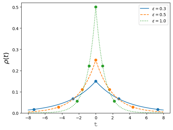
The optimal action $P_{u}$ for a user $u$ , is to add Laplace noise⁵⁵5We use $\mathcal{L}_{\epsilon}(u)$ to denote a Laplace distribution of scale $\frac{1}{\epsilon}$ centred at $u$ . Formally, a distribution $X\sim\mathcal{L}_{\epsilon}(u)$ has its probability density function given by $f_{X}(x)=\frac{\epsilon}{2}e^{-\epsilon|x-u|}$ . of scale $\frac{1}{\epsilon}$ to its value $u$ (result stated in Theorem 19 and proof sketch described in Sections 2.1, 2.2 and 2.3). Further, we emphasize that the optimality of adding Laplace noise is far from obvious⁶⁶6In fact, only a few optimal DP mechanisms are known [39, 43, 46, 25], and it is known that for certain scenarios, universally optimal mechanisms do not exist [17].. For instance, when users and results are located on a ring, Laplace noise is not optimal (see appendix A.2 for an analysis when $k=2$ ).
$\blacksquare$

The optimal server response $\mathbf{Q}$ could be different based on different $\mathfrak{h}$ . We give a recursive construction of $\mathbf{Q}$ for a general $\mathfrak{h}$ (Section 2.4). Furthermore, when $\mathfrak{h}(t)=t$ , we give an exact construction of $\mathbf{Q}$ (sketched in Fig. 2 for $k=5$ ) and show that $f^{\mathds{1}(.)}(\epsilon,k)=O(\frac{1}{\epsilon k})$ in Section 2.4 and [57, Appendix C.5].

Although we do not assume that distributions in $(\mathbf{P},\mathbf{Q})$ admit valid density functions, we prove in Lemma 13 that it suffices to consider only bounded density functions using ideas from mollifier theory [36]. In Appendix A, we generalize our results by allowing user queries to lie on a higher dimensional space and studying $\mathfrak{g}(.)$ -geographic differential privacy (defined in Definition 21) for an increasing convex differentiable function $\mathfrak{g}()$ . Formally, our main results can be stated as:

Theorem 5 (corresponds to Theorem 19 and Theorem C.3 in [41]).

For $\epsilon$ -geographic differential privacy, adding Laplace noise, that is, user $u$ sends a signal drawn from distribution $\mathcal{L}_{\epsilon}(u)$ , is one of the optimal choices of $\mathcal{P}^{(\epsilon)}_{Z}$ for users. Further, when $\mathfrak{h}(t)=t$ , we have $f^{\mathds{1}(.)}(\epsilon,k)=O(\frac{1}{\epsilon k})$ and the optimal mechanism $(Z,\mathbf{P},\mathbf{Q})$ (choice of actions of users and server) itself can be computed in closed form. For a generic $\mathfrak{h}(.)$ , the optimal server action $\mathbf{Q}$ may be computed recursively.

In addition to our overall framework and the tightness of the above theorem, a key contribution of our work is in the techniques developed. At a high level, our proof proceeds via constructing an infinite dimensional linear program to encode the optimal algorithm under DP constraints. We then use dual fitting to show the optimality of Laplace noise. Finally, the optimal set of results being computable by a simple dynamic program given such noise.

The technical hurdles arise because the linear program for encoding the optimal mechanism is over infinite-dimensional function spaces with linear constraints on both derivatives and integrals, since the privacy constraint translates to constraints on the derivative of the density encoding the optimal mechanism, while capturing the density itself requires an integral. We call it Differential Integral Linear Program (DILP); see Section 2.2. However, there is no weak duality theory for such linear programs in infinite dimensional function spaces, such results only existing for linear programs with integral constraints [3]. We, therefore, develop a weak duality theory for DILPs (see Section 2.2 with a detailed proof in [41, Appendix C.6]), which to the best of our knowledge is novel. The proof of this result is quite technical and involves a careful application of Fatou’s lemma [56] and the monotone convergence theorem to interchange integrals with limits, and integration by parts to translate the derivative constraints on the primal variables to derivatives constraint on the dual variables. We believe our weak duality framework is of independent interest and has broader implications beyond differential privacy; see [41, Appendix B.7] for two such applications.

Refer to caption — Figure 2: Optimal mechanisms in geographic differential privacy setting when $k=5$ and $\epsilon\in\{0.3,0.5,1.0\}$ . Suppose the user has a private value $u$ . Then the user sends a signal $s$ drawn from distribution $\mathcal{L}_{\epsilon}(u)$ to the server, meaning the user sends $s=v+x$ where $x$ is drawn from the density function $\rho(t)$ in this figure. Suppose the server receives $s$ . Then the server responds $\{s+a_{1},...,s+a_{5}\}$ , where the values of $a_{1},a_{2},...,a_{5}$ are the $t$ -axis values of dots on the density functions.

1.3 Related Work

1.3.1 Differential Privacy

The notion of differential privacy in the trusted curator model is introduced in [27]; see [29] for a survey of foundational results in this model. The idea of local differential privacy dates back to [47], and the algorithms for satisfying it have been studied extensively following the deployment of DP in this model by Google [31] and Apple [6]; see, e.g. [18, 21, 60, 11] and Bebensee [13] for a survey. Geographic differential privacy was introduced by [4] and has gained widespread adoption for location data. Since GDP utilizes the trust assumptions of the local model, it is only a slight relaxation of the traditional local model of DP.

1.3.2 Multi-Selection

An architecture for multi-selection, particularly with the goal of privacy-preserving advertising, was introduced in Adnostic by [58]. Their proposal was to have a browser extension that would run the targeting and ad selection on the user’s behalf, reporting to the server only click information using cryptographic techniques. Similarly, Privad by [42] propose to use an anonymizing proxy that operates between the client that sends broad interest categories to the proxy and the advertising broker, that transmits all ads matching the broad categories, with the client making appropriate selections from those ads locally. Although both Adnostic and Privad reason about the privacy properties of their proposed systems, unlike our work, neither provides DP guarantees.

Two lines of work in the DP literature can be seen as related to the multi-selection paradigm – the exponential mechanism (see e.g. [52, 16, 50]) and amplification by shuffling (see e.g. [30, 22, 33]). The exponential mechanism focuses on high-utility private selection from multiple alternatives and is usually deployed in the Trusted Curator Model (TCM). Amplification by shuffling analyzes the improvement in the DP guarantees that can be achieved if the locally privatized data is shuffled by an entity before being shared with the server. As far as we are aware, neither of the results from these lines of work can be directly applied to our version of multi-selection, although combining them is an interesting avenue for future work.

Several additional directions within DP research can be viewed as exploring novel system architectures in order to improve privacy-utility trade-offs, e.g., using public data to augment private training [53, 10], combining data from TCM and LM models [8, 7, 14], and others. Our proposed architecture is distinct from all of these. Finally, our work is different from how privacy is applied in federated learning [38] – there, the goal is for a centralized entity to be able to build a machine learning model based on distributed data; whereas our goal is to enable personalized, privacy-preserving retrieval from a global ML model.

The closest work we are aware of is Apple’s very recent system using multiple options presented to users to improve its generation of synthetic data using DP-user feedback [55].

1.3.3 Optimal DP mechanisms

To some extent, previous work in DP can be viewed as searching for the optimal DP mechanism, i.e. one that would achieve the best possible utility given a fixed desired DP level. Only a few optimal mechanisms are known [39, 43, 46, 25], and it is known that for certain scenarios, universally optimal mechanisms do not exist [17]. Most closely related to our work is the foundational work of [39] that derives the optimal mechanism for counting queries via a linear programming formulation; the optimal mechanism turns out to be the discrete version of the Laplace mechanism. Its continuous version was studied in [34], where the Laplace mechanism was shown to be optimal. These works focused on the trusted curator model of differential privacy unlike the local trust model which we study.

In the local model, [49] show Laplace noise to be optimal for $\epsilon$ -geographic DP. Their proof relies on formulating an infinite dimensional linear program over noise distributions and looking at its dual. Although their proof technique bears a slight resemblance to ours, our proof is different and intricate since it involves the minimisation over the set of returned results in the cost function. A variation of local DP is considered in [37], in which DP constraints are imposed only when the distance between two users is smaller than a threshold. For that setting, the optimal noise is piece-wise constant. However, our setting of choosing from multiple options makes the problems very different.

1.3.4 Homomorphic encryption

Recent work of [45] presents a private web browser where users submit homomorphically encrypted queries, including the cluster center $i^{*}$ and search text $q$ . The server computes the cosine similarity between $q$ and every document in cluster $i^{*}$ , allowing the user to select the index of the most similar document. To retrieve the URL, private information retrieval [24] is used. This approach requires making all cluster centers public and having the user identify the closest $i^{*}$ , which differs significantly from our multi-selection model.

Additionally, homomorphic encryption for machine learning models [51, 23] faces practical challenges, such as high computational overhead and reduced utility, limiting real-world deployment. While our multi-selection framework provides a weaker privacy guarantee than homomorphic encryption, it avoids requiring the recommendation service to publish its full data or index, which in certain context may be viewed as proprietary information by the service. We thus argue that homomorphic encryption-based and multi-selection based approaches offer distinct trade-offs, making them complementary tools for private recommendation systems.

1.3.5 Related work on duality theory for infinite dimensional LPs

Strong duality is known to hold for finite dimensional linear programs [19]. However, for infinite dimensional linear programs, strong duality may not always hold (see [3] for a survey). Sufficient conditions for strong duality are presented and discussed in [59, 12] for generalized vector spaces. A class of linear programs (called SCLPs) over bounded measurable function spaces have been studied in [54, 15] with integral constraints on the functions. However, these works do not consider the case with derivative constraints on the functional variables. In [49, Equation 7] a linear program with derivative and integral constraints (DILPs) is formulated to show the optimality of Laplace noise for geographic differential privacy. However, their duality result does not directly generalize to our case since our objective function and constraints are far more complex as it involves minimization over a set of results.

We thus need to reprove the weak-duality theorem for our DILPs, the proof of which is technical and involves a careful application of integration by parts to translate the derivative constraint on the primal variable to a derivative constraint on the dual variable. Further, we require a careful application of Fatou’s lemma [56] and monotone convergence theorem to exchange limits and integrals. Our weak duality result generalizes beyond our specific example and is applicable to a broader class of DILPs. Furthermore, we discuss two problems (one from job scheduling [2] and one from control theory [32]) in [41, Appendix B.7] which may be formulated as a DILP.

2 Characterizing the Optimal Mechanism: Proof Sketch of Theorem 5

We now present a sketch of the proof of Theorem 5; the full proof involving the many technical details is presented in the Appendix. We first show that for the sake of analysis, the server can be removed by making the signal set coincide with result sets (Section 2.1) assuming that the function OPT is publicly known both to the user and server.⁷⁷7One should note that this removal is just for analysis and the server is needed since the OPT function is unknown to the user. Then in Section 2.2 we construct a primal linear program $\mathcal{O}$ for encoding the optimal mechanism, and show that it falls in a class of infinite dimensional linear programs that we call DILPs, as defined below.

Definition 6.

Differential-integral linear program (DILP) is a linear program over Riemann integrable function spaces involving constraints on both derivatives and integrals.

A simple example is given in Equation (9). Observe that in equation (9), we define $\mathcal{C}_{1}$ to be a continuously differentiable function.

{}\text{\Large{$\tilde{\mathcal{O}}=$} }\left\{\begin{aligned} \inf_{g(.):% \mathcal{C}^{1}(\mathbb{R}\rightarrow\mathbb{R}^{+})}&\int_{\mathbb{R}}|v|g(v)% dv\\ \textrm{s.t.}\quad&\int_{\mathbb{R}}g(v)dv=1\\ &-\epsilon g(v)\leq g^{\prime}(v)\leq\epsilon g(v)\text{ }\forall v\in\mathbb{% R}\end{aligned}\right.

(9)

We next construct a dual DILP formulation $\mathcal{E}$ in Section 2.2, and show that the formulation satisfies weak duality. As mentioned before, this is the most technically intricate result since we need to develop a duality theory for DILPs. We relegate the details of the proof here to the Appendix.

Next, in Section 2.3, we show the optimality of the Laplace noise mechanism via dual-fitting, i.e., by constructing a feasible solution to DILP $\mathcal{E}$ with objective identical to that of the Laplace noise mechanism. Finally, in Section 2.4, we show how to find the optimal set of $k$ results given Laplace noise. We give a construction for general functions $\mathfrak{h}(.)$ as well as a closed form for the canonical case of $\mathfrak{h}(t)=t$ . This establishes the error bound and concludes the proof of Theorem 5.

2.1 Restricting the signal set $𝒁$ to $\mathbb{R}^{k}$

We first show that it is sufficient to consider a more simplified setup where the user sends a signal set in ^k and the server sends back the results corresponding to the signal set. Since we assumed users and results lie in the same set, for the purpose of analysis, this removes the server from the picture. To see this, note that for the setting discussed in Section 1.1.4, the optimal result for user $u$ is the result $u$ itself, where when we refer to “result $u$ ”, we refer to the result $\text{OPT}(u)\in M$ .

Thus, this approach is used only for a simplified analysis as the OPT function is not known to the user and our final mechanism will actually split the computation between the user and the server.

Therefore a user can draw a result set directly from the distribution over the server’s action and send the set as the signal. The server returns the received signal, hence removing it from the picture. In other words, it is sufficient to consider mechanisms in $\mathcal{P}^{(\epsilon)}_{\real{}^{k}}$ , which are in the following form (corresponding to Theorem 8).

1.

User $v\in\real$ reports $s$ that is drawn from a distribution $P_{v}$ over ^k.
2.

The server receives $s$ and returns $s$ .

We give an example to illustrate this statement below.

Example 7.

Fix a user $u$ and let $Z=\{s_{1},s_{2}\}$ and $\{\textbf{a}^{(1)},\textbf{a}^{(2)}\}\subseteq\mathbb{R}^{k}$ and consider a mechanism $\mathcal{M}_{1}$ where user $u$ sends $s_{1}$ and $s_{2}$ with equal probability. The server returns $\textbf{a}\in\real^{k}$ on receiving signal $s$ , with the following probability.

	$\displaystyle\operatorname{\mathbb{P}}\left(\textbf{a}=\textbf{a}^{(1)}\|s=s_{1% }\right)=0.2,\quad\operatorname{\mathbb{P}}\left(\textbf{a}=\textbf{a}^{(2)}\|s% =s_{1}\right)=0.8,$
	$\displaystyle\operatorname{\mathbb{P}}\left(\textbf{a}=\textbf{a}^{(1)}\|s=s_{2% }\right)=0.4,\quad\operatorname{\mathbb{P}}\left(\textbf{a}=\textbf{a}^{(2)}\|s% =s_{2}\right)=0.6.$

Then the probability that $u$ receives $\textbf{a}^{(1)}$ is 0.3 and it receives $\textbf{a}^{(2)}$ is 0.7. Now consider another mechanism $\mathcal{M}_{2}$ with the same cost satisfying differential privacy constraints, where $Z=\{\textbf{a}^{(1)},\textbf{a}^{(2)}\}$ , with user $u$ sending signal $\textbf{a}^{(1)}$ and $\textbf{a}^{(2)}$ with probabilities 0.3 and 0.7. When the server receives $\textbf{a}\in\real^{k}$ , it returns a.

We show the new mechanism $\mathcal{M}_{2}$ satisfies differential privacy assuming the original mechanism $\mathcal{M}_{1}$ satisfies it. As a result, we can assume $Z=\real^{k}$ when finding the optimal mechanism.

The following theorem states that it is sufficient to study a setup removing the server from the picture and consider mechanisms in set of probability distributions supported on ^k satisfying $\epsilon$ -geographic differential privacy ( $\mathcal{P}^{(\epsilon)}_{\real{}^{k}}$ as defined in Section 1.1.5).

Theorem 8 (detailed proof in Appendix C.1 of [41]).

It is sufficient to remove the server $(\mathbf{Q})$ from the cost function $f^{\mathfrak{h}(.)}(\epsilon,k)$ and pretend the user has full-information. Mathematically, it maybe stated as follows.

{}f^{\mathfrak{h}(.)}(\epsilon,k)=\inf_{\mathbf{P}\in\mathcal{P}^{(\epsilon)}_% {\real{}^{k}}}\sup_{u\in\real}\mathop{\operatorname{\mathbb{E}}}\limits_{% \textbf{a}\sim P_{u}}\left[\min_{a\in\texttt{Set}(\textbf{a})}\mathfrak{h}(|u-% a|)\right].

(10)

Proof Sketch.

Fix $Z,\mathbf{P}\in\mathcal{P}^{(\epsilon)}_{Z},\mathbf{Q}\in\mathcal{Q}_{Z}$ . For $u\in\real$ and $S\subseteq\real^{k}$ , let $\tilde{P}_{u}\left(S\right)$ be the probability that the server returns a set in $S$ to user $u$ . Then for any $u_{1},u_{2}\in\real,S\subseteq\real^{k}$ , we can show that $\tilde{P}_{u_{1}}\left(S\right)\leq e^{\epsilon\cdot|u_{1}-u_{2}|}\tilde{P}_{u% _{2}}\left(S\right)$ using post-processing theorem, and thus $\tilde{\mathbf{P}}=\{\tilde{P}_{u}\}_{u\in\real}\in\mathcal{P}^{(\epsilon)}_{% \real{}^{k}}$ because $\tilde{P}_{u}$ is a distribution on ^k for any $u\in\real$ . At the same time,

\displaystyle\mathop{\operatorname{\mathbb{E}}}\limits_{s\sim P_{u}}\left[% \mathop{\operatorname{\mathbb{E}}}\limits_{\textbf{a}\sim Q_{s}}\left[\min_{a% \in\texttt{Set}(\textbf{a})}\mathfrak{h}(|u-a|)\right]\right]=\mathop{% \operatorname{\mathbb{E}}}\limits_{\textbf{a}\sim\tilde{P}_{u}}\left[\min_{a% \in\texttt{Set}(\textbf{a})}\mathfrak{h}(|u-a|)),\right]\text{ so we have}

\displaystyle f^{\mathfrak{h}(.)}(\epsilon,k)=\inf_{\mathbf{P}\in\mathcal{P}^{% (\epsilon)}_{\real{}^{k}}}\sup_{u\in\real}\mathop{\operatorname{\mathbb{E}}}% \limits_{\textbf{a}\sim P_{u}}\left[\min_{a\in\texttt{Set}(\textbf{a})}% \mathfrak{h}(|u-a|)\right].

$\hfill\blacktriangleleft$

2.2 Differential integral linear programs to represent $f(\epsilon,k)$ and a weak duality result

Recall the definition of DILP from Definition 6. In this section, we construct an infimizing DILP $\mathcal{O}$ to represent the constraints and the objective in the cost function $f(\epsilon,k)$ . We then construct a dual DILP $\mathcal{E}$ , and provide some intuition for this formulation. The proof of weak duality is our main technical result, and its proof is defered to the Appendix.

2.2.1 Construction of DILP $\mathcal{O}$ to represent cost function $f(\epsilon,k)$

We now define the cost of a mechanism $\mathbf{P}$ which overloads the cost definition in Equation 6

Definition 9.

Cost of mechanism $\textbf{P}\in\mathcal{P}^{(\epsilon)}_{\mathbb{R}^{k}}$ : We define the cost of mechanism P as

{}\textit{cost}(\textbf{P}):=\sup_{u\in\mathbb{R}}\underset{\textbf{a}\sim P_{% u}}{\mathbb{E}}\left[\min_{a\in\texttt{Set}(\textbf{a})}\mathfrak{h}(|u-a|)\right]

(11)

Observe that in Definition 9 we just use $\mathbf{P}$ instead of the tuple $(Z,\mathbf{P},\mathbf{Q})$ as in Equation (6). Observe that it is sufficient to consider $\mathbf{P}$ in the cost since $\mathbf{P}$ simulates the entire combined action of the user and the server as shown in Theorem 10 in Section 2.1. We now define the notion of approximation using cost of mechanism by a sequence of mechanisms which is used in the construction of DILP $\mathcal{O}$ .

Definition 10.

Arbitrary cost approximation: We call mechanisms $\textbf{P}^{(\eta)}\in\mathcal{P}^{(\epsilon)}_{\mathbb{R}^{k}}$ an arbitrary cost approximation of mechanisms $\textbf{P}\in\mathcal{P}^{(\epsilon)}_{\mathbb{R}^{k}}$ if $\lim\limits_{\eta\to 0}\textit{cost}(\textbf{P}^{(\eta)})=\textit{cost}(% \textbf{P})$

Now we define the DILP $\mathcal{O}$ to characterise ${f}(\epsilon,k)$ in Equation (10). In this formulation, the variables are $g(.,.):\mathcal{I}^{B}(\mathbb{R}\times\mathbb{R}^{k}\rightarrow\mathbb{R}^{+})$ , which we assume are non-negative Riemann integrable bounded functions. These variables capture the density function $P_{u}$ .

{}\text{ \Large{$\mathcal{O}=$}}\left\{\begin{aligned} \inf_{g(.,.):\mathcal{I% }^{B}(\mathbb{R}\times\mathbb{R}^{k}\rightarrow\mathbb{R}^{+}),\kappa\in% \mathbb{R}}\quad&\kappa\\ \textrm{s.t.}\quad&\kappa-\int\limits_{\textbf{x}\in\mathbb{R}^{k}}\left[\min_% {a\in\texttt{Set}(\textbf{x})}\mathfrak{h}(|u-a|)\right]g(u,\textbf{x})d\left(% \prod_{i=1}^{k}x_{i}\right)\geq 0\text{ }\forall u\in\mathbb{R}\\ &\int\limits_{\textbf{x}\in\mathbb{R}^{k}}g(u,\textbf{x})d\left(\prod_{i=1}^{k% }x_{i}\right)=1\text{ }\forall u\in\mathbb{R}\\ &\epsilon g(u,\textbf{x})+\underline{g}_{u}(u,\textbf{x})\geq 0;\text{ }% \forall u\in\mathbb{R};\textbf{x}\in\mathbb{R}^{k}\\ &\epsilon g(u,\textbf{x})-\overline{g}_{u}(u,\textbf{x})\geq 0;\text{ }\forall u% \in\mathbb{R};\textbf{x}\in\mathbb{R}^{k}\end{aligned}\right.

(12)

In DILP $\mathcal{O}$ , we define $\underline{g}_{u}(u,\textbf{x})$ and $\overline{g}_{u}(u,\textbf{x})$ to be the lower and upper partial derivative of $g(u,\textbf{x})$ at $u$ . Now observe that, we use lower and upper derivatives instead of directly using derivatives as the derivatives of a probability density function may not always be defined (for example, the left and right derivatives are unequal in the Laplace distribution at origin).

Note that the DILP $\mathcal{O}$ involves integrals and thus requires mechanisms to have a valid probability density function, however not every distribution is continuous, and, as a result, may not have a density function (e.g. point mass distributions like $\hat{P}^{\mathcal{L}_{\epsilon}}_{u}$ defined in Definition 15). Using ideas from mollifier theory [35] we construct mechanisms $\textbf{P}^{(\eta)}$ with a valid probability density function that are an arbitrary good approximation of mechanism P in Lemma 13, hence showing that it suffices to define $\mathcal{O}$ over bounded, non-negative Reimann integrable functions $g$ . We now prove that the DILP constructed above captures the optimal mechanism, in other words, $\text{opt}(\mathcal{O})=f(\epsilon,k)$ .

Lemma 11.

Let $\text{opt}(\mathcal{O})$ denote the optimal value of DILP (12), then $f(\epsilon,k)=\text{opt}(\mathcal{O})$ .

To prove this lemma, we show Lemma 12, which relates the last two constraints of the DILP $\mathcal{O}$ to $\epsilon$ -geographic differential privacy, and Lemma 13, which shows that an arbitrary cost approximation of mechanism P can be constructed with valid probability density functions.

Lemma 12.

Let $P_{u}$ have a probability density function given by $g(u,.):\mathbb{R}^{k}\rightarrow\mathbb{R}$ for every $u\in\mathbb{R}$ . Then, $\mathbf{P}$ satisfies $\epsilon$ -geographic differential privacy iff $\max(|\overline{g}_{u}(u,\textbf{x})|,|\underline{g}_{u}(u,\textbf{x})|)\leq% \epsilon g(u,\textbf{x})\text{ }\forall u\in\mathbb{R};\forall\textbf{x}\in% \mathbb{R}^{k}$ ⁸⁸8 $\underline{g}_{u}(u,\textbf{x})$ , $\overline{g}_{u}(u,\textbf{x})$ denote the lower and upper partial derivative w.r.t. $u$

The proof of this lemma ([41, Appendix C.2.1]) proceeds by showing that $\epsilon$ -geographic differential privacy is equivalent to Lipschitz continuity of $\log g(u,\textbf{x})$ in $u$ .⁹⁹9We handle the case when the $\log$ is not defined as the density is zero at some point separately in the proof.

Lemma 13.

(Proven in [41, Appendix C.2.5]) Given any mechanism $\textbf{P}\in\mathcal{P}^{(\epsilon)}_{\textbf{R}^{k}}$ (satisfying $\epsilon$ -geographic differential privacy), we can construct a sequence of mechanisms $\textbf{P}^{(\eta)}$ with bounded probability density functions such that $\textbf{P}^{(\eta)}$ is an arbitrary cost approximation of mechanism $\textbf{P}\in\mathcal{P}^{(\epsilon)}_{\textbf{R}^{k}}$ .

Using Lemmas 13 and 12, we give the proof of Lemma 11.

Proof of Lemma 11.

Consider any $\zeta>0$ . As established in Lemma 13, it follows for every mechanism $\textbf{P}\in\mathcal{P}^{(\epsilon)}_{\textbf{R}^{k}}$ , we can construct another mechanism $\textbf{P}^{(\eta)}$ with bounded probability density functions whose cost is a $\zeta$ approximation of the cost of mechanism P. Thus, we can use Lemma 12 to conclude that the optimum value of DILP $\mathcal{O}$ is precisely $f(\epsilon,k)$ . $\hfill\blacktriangleleft$

2.2.2 Dual DILP $\mathcal{E}$ and statement of weak duality theorem

Now, we write the dual of the DILP $\mathcal{O}$ as the DILP $\mathcal{E}$ in Equation (13). Observe that, we have the constraint that $\delta(.)$ and $\lambda(.)$ is non-negative, $\mathcal{C}^{0}$ (continuous) and $\nu(.,.)$ is a $\mathcal{C}^{1}$ function i.e. $\nu(r,\textbf{v})$ is continuously differentiable in $r$ and continuous in v. Thus, we may rewrite the equations as

{}\text{\Large{$\mathcal{E}=$} }\left\{\begin{aligned} \sup_{\begin{subarray}{% c}\delta(.),\lambda(.):\mathcal{C}^{0}(\mathbb{R}\rightarrow\mathbb{R}^{+});\\ \nu(.,.):\mathcal{C}^{1}(\mathbb{R}\times(\mathbb{R})^{k}\rightarrow\mathbb{R}% )\end{subarray}}&\int_{r\in\mathbb{R}}\lambda(r)dr\\ \textrm{s.t. }\quad&\int_{r\in\mathbb{R}}\delta(r)dr\leq 1\\ &\hskip-27.00005pt-\left[\min_{a\in\texttt{Set}(\textbf{v})}\mathfrak{h}(|r-a|% )\right]\delta(r)+\lambda(r)+\nu_{r}(r,\textbf{v})+\epsilon|\nu(r,\textbf{v})|% \leq 0\text{ }\forall r\in\mathbb{R};\textbf{v}\in(\mathbb{R})^{k}\\ &\exists U:\mathcal{C}^{0}(\mathbb{R}^{k}\rightarrow\mathbb{R})\textrm{ s.t. }% \nu(r,\textbf{v})\geq 0\text{ }\forall r\geq U(\textbf{v})\text{ }\forall% \textbf{v}\in(\mathbb{R})^{k}\\ &\exists L:\mathcal{C}^{0}(\mathbb{R}^{k}\rightarrow\mathbb{R})\textrm{ s.t. }% \nu(r,\textbf{v})\leq 0\text{ }\forall r\leq L(\textbf{v})\text{ }\forall% \textbf{v}\in(\mathbb{R})^{k}\end{aligned}\right.

(13)

To get intuition behind the construction of our dual DILP $\mathcal{E}$ , relate the equations in DILP $\mathcal{O}$ to the dual variables of DILP $\mathcal{E}$ as follows. The first equation denoted by $\{\delta(r)\}_{r\in\mathbb{R}}$ , second equation denoted by $\{\lambda(r)\}_{r\in\mathbb{R}}$ and the last two equations are jointly denoted by $\{\nu(r,\textbf{v})\}_{r\in\mathbb{R};\textbf{v}\in(\mathbb{R})^{k}}$ ¹⁰¹⁰10Note that the variable $\nu(r,\textbf{v})$ is constructed from the difference of two non-negative variables corresponding to third and fourth equations, respectively. The detailed proof is in [41, Appendix C.6]. The last two terms in the second constraint of DILP $\mathcal{E}$ are a consequence of the last two equations on DILP $\mathcal{O}$ and observe that it involves a derivative of the dual variable $\nu(u,\textbf{v})$ . The linear constraint on the derivative of the primal variable translates to a derivative constraint on the dual variable by a careful application of integration by parts, discussed in detail in [41, Appendix C.6].

Observe that in our framework we have to prove the weak-duality result as, to the best of our knowledge, existing duality of linear programs in infinite dimensional spaces work for cases involving just integrals. The proof of this Theorem 14 is technical and we defer the details to [41, Appendix C.6].

Theorem 14.

$\text{opt}(\mathcal{O})\geq\text{opt}(\mathcal{E})$ .

2.3 Dual fitting to show the optimality of Laplace noise addition

Before starting this section, we first define a function $\hat{f}(\epsilon,k)$ which characterises the optimal placement of $k$ points in to minimise the expected minimum disutility among these $k$ points measured with respect to some user $u$ sampled from a Laplace distribution. As we shall prove in Theorem 16 that it bounds the cost of the Laplace noise addition mechanism.

{}\hat{f}(\epsilon,k)=\min_{\textbf{a}\in\mathbb{R}^{k}}\mathop{\operatorname{% \mathbb{E}}}\limits_{y\sim\mathcal{L}_{\epsilon}(0)}\left[\min_{a\in\texttt{% Set}(\textbf{a})}\mathfrak{h}(|y-a|)\right]

(14)

In this section, we first define a mechanism in Definition 15 which simulates the action of the server corresponding to the Laplace noise addition mechanism in Section 2.3.1 and show that the cost of Laplace noise addition mechanism is $\hat{f}(\epsilon,k)$ . We finally show the optimality of Laplace noise addition mechanism via dual fitting i.e. constructing a feasible solution to the dual DILP $\mathcal{E}$ with an objective function $\hat{f}(\epsilon,k)$ in Section 2.3.2.

2.3.1 Bounding cost function $f(\epsilon,k)$ by the cost of Laplace noise adding mechanism

We now define the mechanism $\hat{\textbf{P}}^{\mathcal{L}_{\epsilon}}=\{\hat{P}_{u}^{\mathcal{L}_{\epsilon% }}\}_{u\in\real}$ which corresponds to simulating the action of the server on receiving signal $S_{u}\sim\mathcal{L}_{\epsilon}(u)$ from user $u$ . We often call this in short as the Laplace noise addition mechanism.

Definition 15.

The distribution $\hat{P}^{\mathcal{L}_{\epsilon}}_{u}$ is defined as follows for every $u\in\real$ .

	$\displaystyle{}\hat{\textbf{a}}\sim\hat{P}^{\mathcal{L}_{\epsilon}}_{u}\iff% \hat{\textbf{a}}=$	$\displaystyle\operatorname*{arg\,min}_{\textbf{a}\in\mathbb{R}^{k}}\mathop{% \operatorname{\mathbb{E}}}\limits_{y\sim\mathcal{L}_{\epsilon}(S_{u})}\left[% \min_{a\in\texttt{Set}(\textbf{a})}\mathfrak{h}(\|y-a\|)\right]\text{ where }S_{% u}\sim\mathcal{L}_{\epsilon}(u)$		(15)
	$\displaystyle\overset{(a)}{=}$	$\displaystyle\operatorname*{arg\,min}_{\textbf{a}\in\mathbb{R}^{k}}\mathop{% \operatorname{\mathbb{E}}}\limits_{y\sim\mathcal{L}_{\epsilon}(0)}\left[\min_{% a\in\texttt{Set}(\textbf{a})}\mathfrak{h}(\|y-a\|)\right]+S_{u}\text{where }S_{u% }\sim\mathcal{L}_{\epsilon}(u)$		(16)

Equality $(a)$ follows from the fact that $y\sim\mathcal{L}_{\epsilon}(z)\implies y-z\sim\mathcal{L}_{\epsilon}(0)$ for every $z\in\mathbb{R}$ .

Observe that the server responds with set of points $\texttt{Set}(\textbf{a})$ for some $\textbf{a}\in\mathbb{R}^{k}$ so as to minimise the expected cost with respect to some user sampled from a Laplace distribution centred at $S_{u}$ . We show that the following lemma which states that $\hat{P}^{\mathcal{L}_{\epsilon}}$ satisfies $\epsilon$ -geographic differential privacy constraints and bound $f(\epsilon,k)$ by $\hat{f}(\epsilon,k)$ .

Lemma 16 (detailed proof in Appendix C.3 of [41]).

$\hat{\textbf{P}}^{\mathcal{L}_{\epsilon}}$ satisfies $\epsilon$ -geographic differential-privacy constraints i.e. $\hat{\textbf{P}}^{\mathcal{L}_{\epsilon}}\in\mathcal{P}^{(\epsilon)}_{\mathbb{% R}^{k}}$ and thus, we have $f(\epsilon,k)\leq\textit{cost}(\hat{{P}}^{\mathcal{L}_{\epsilon}})=\hat{f}(% \epsilon,k)$

Proof Sketch.

Observe that $\hat{P}^{\mathcal{L}_{\epsilon}}\in\mathcal{P}^{(\epsilon)}_{\mathbb{R}^{k}}$ from the post processing theorem, refer to [28] since $S_{u}\sim\mathcal{L}_{\epsilon}(u)$ satisfies $\epsilon$ -geographic differential privacy constraints.¹²¹²12Post processing theorem can be proven even for $\epsilon$ -geographic differential privacy similarly.. Thus, we prove $f(\epsilon,k)\leq\text{cost}(\hat{{P}}^{\mathcal{L}_{\epsilon}})$ . The equality is fully proven in [57, Appendix C.3]. $\hfill\blacktriangleleft$

2.3.2 Obtaining a feasible solution to DILP $\mathcal{E}$

We now construct feasible solutions to DILP $\mathcal{E}$ . For some $\zeta>0$ and $\hat{\lambda}>0$ , we define

{}\delta^{(c)}(r)=(\zeta/2)e^{-\zeta|r|}\text{ and }\lambda^{(c)}(r)=\hat{% \lambda}\cdot(\zeta/2)e^{-\zeta|r|}\text{ }\forall r\in\mathbb{R}

(17)

Now define $v_{med}=\text{Median}(\texttt{Set}(\textbf{v}))$ and for every $\textbf{v}\in\mathbbm{R}^{k}$ , we consider the following Differential Equation (18) in $\hat{\nu}(.)$ .

{}-\left[\min_{a\in\texttt{Set}(\textbf{v})}\mathfrak{h}(|r-a|)\right]\delta^{% (c)}(r)+\lambda^{(c)}(r)+\frac{d\hat{\nu}(r)}{dr}+\epsilon|\hat{\nu}(r)|=0;% \text{ with $\hat{\nu}(v_{med})=0$}

(18)

Observe that this equation precisely corresponds to the second constraint of DILP $\mathcal{E}$ (inequality replaced by equality) with an initial value. We now show that a solution $\hat{\nu}(.)$ to differential equation (18) exists such that $\hat{\nu}(r)$ is non-negative for sufficiently large $r$ and non-positive for sufficiently small $r$ to satisfy the last two constraints of DILP $\mathcal{E}$ in Lemma 17. Observe that the structure of our differential equation is similar to that in [49, Equation 19]. However, our differential equation has significantly more complexity since we are minimising over a set of points $\textbf{v}\in\mathbb{R}^{k}$ and also our equation has to be solved for every $\textbf{v}\in\mathbb{R}^{k}$ making it more complex.

Lemma 17 (Proof in Appendix C.4.2 of [41]).

Choose $\zeta<\epsilon$ and $0<\hat{\lambda}\leq\frac{\epsilon-\zeta}{\epsilon+\zeta}\hat{f}(\epsilon+\zeta% ,k)$ , then equation $\eqref{eqn:diff_eqn_nu}$ has a unique $\mathcal{C}^{1}$ solution $\nu^{(c)}(.)$ and there exists $U,L\in\mathbb{R}$ satisfying $\nu^{(c)}(r)\geq 0\text{ }\forall r\geq U$ and $\nu^{(c)}(r)\leq 0\text{ }\forall r\leq L$ .

Intuitive explanation.

We just give an intuition for this proof for the case where $\hat{\lambda}$ exceeds $\frac{\epsilon-\zeta}{\epsilon+\zeta}\hat{f}(\epsilon,k)$ by showing two plots in Figure 3(a) and 3(b) for the two cases where $\hat{\lambda}<\frac{\epsilon-\zeta}{\epsilon+\zeta}\hat{f}(\epsilon,k)$ and $\hat{\lambda}>\frac{\epsilon-\zeta}{\epsilon+\zeta}\hat{f}(\epsilon,k)$ respectively. In the first case, $\nu^{(c)}(r)$ is positive for sufficiently large $r$ and in second case, it goes negative for large $r$ demonstrating the requirement of the bound $\frac{\epsilon-\zeta}{\epsilon+\zeta}\hat{f}(\epsilon,k)$ on $\hat{\lambda}$ . The two plots are for the case when $\epsilon=1$ , $\zeta=0.1$ , $\mathfrak{h}(z)=z$ and thus $\frac{\epsilon-\zeta}{\epsilon+\zeta}\hat{f}(\epsilon,k)$ may be approximately by $\frac{9}{11}\times\frac{1}{2}=0.44$ as shown in Section 2.4. For the purpose of the plots, we choose $\textbf{v}=[-\log 4;\text{ }0;\text{ }\log 4]^{T}$ ¹³¹³13We choose this vector as it minimises equation (14) with detailed calculation is given in Section 2.4. and demonstrate the point in the Lemma.

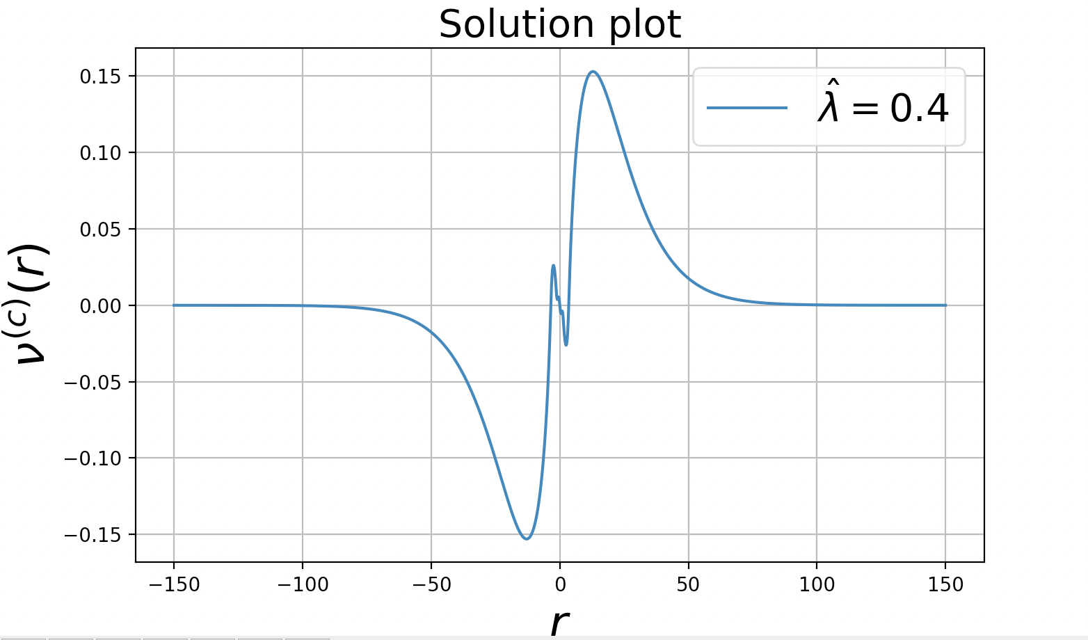
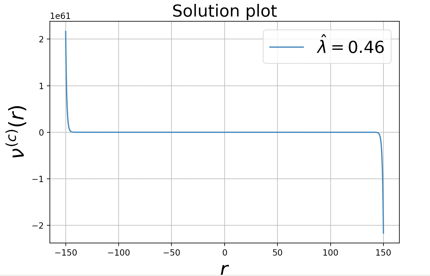
These spikes in the solution may be observed due to the selection of $\textbf{v}\in\mathbb{R}^{3}$ due to the term $\left[\min\limits_{a\in\texttt{Set}(\textbf{v})}\mathfrak{h}(|r-a|)\right]$ in the differential equation. $\hfill\blacktriangleleft$

Lemma 18 (detailed proof in Appendix C.4.2 of [41]).

$\text{opt}(\mathcal{E})\geq\hat{f}(\epsilon,k)$ .

We present a proof sketch where we do not explicitly show the continuity of the bounds $U(.)$ and $L(.)$ . In [41, Appendix C.7], we prove a claim showing such an existence.

Proof Sketch.

Recall the functions $\lambda^{(c)}(.),\delta^{(c)}(.)$ defined in (17). Also for every $\textbf{v}\in\mathbb{R}^{k}$ , we obtain a function $\nu^{(c)}(.,\textbf{v})$ [solution of Equation (18)] with bounds $U(\textbf{v})$ and $L(\textbf{v})$ satisfying $\nu^{(c)}(r,\textbf{v})\geq 0\text{ }\forall u\geq U(\textbf{v})$ and $\nu^{(c)}(r,\textbf{v})\leq 0\text{ }\forall u\leq L(\textbf{v})$ and this solution is feasible.

The objective value of this feasible solution is $\hat{\lambda}$ and the constructed solution is feasible for any $\hat{\lambda}\leq\frac{\epsilon-\zeta}{\epsilon+\zeta}\hat{f}(\epsilon+\zeta,k)$ and $\zeta>0$ . Now, since $\hat{f}(\epsilon,k)$ is continuous in $\epsilon$ , choosing $\zeta$ to be arbitrarily small enables us to obtain the objective value of the solution arbitrarily close to $\hat{f}(\epsilon,k)$ and thus, $\text{opt}(\mathcal{E})\geq\hat{f}(\epsilon,k)$ . $\hfill\blacktriangleleft$

Observe that although we defined the Laplace noise addition mechanism $(\hat{\textbf{P}}^{\mathcal{L}_{\epsilon}})$ (see Definition 15) entirely in terms of the user’s action, we can consider an alternate mechanism splitting $(\hat{\textbf{P}}^{\mathcal{L}_{\epsilon}})$ into user’s action and server’s response attaining the same cost:

$\blacksquare$

User $u$ sends $S_{u}\sim\mathcal{L}_{\epsilon}(u)$ to the server.
$\blacksquare$

The server on receiving $S_{u}$ responds with a vector $\textbf{a}=\operatorname*{arg\,min}\limits_{\textbf{a}\in\real^{k}}\mathop{% \operatorname{\mathbb{E}}}\limits_{y\sim\mathcal{L}_{\epsilon}(S_{u})}\left[% \min\limits_{a\in\texttt{Set}(\textbf{a})}\mathfrak{h}(|y\!-\!a|)\right]$ .

Theorem 19.

For $\epsilon$ -geographic differential privacy, sending Laplace noise, that is, user $u$ sends a signal drawn from distribution $\mathcal{L}_{\epsilon}(u)$ is one of the optimal choices of $\mathcal{P}^{(\epsilon)}_{Z}$ for users, and in this case $f^{\mathfrak{h}(.)}(\epsilon,k)=\hat{f}(\epsilon,k)$ .

Proof.

Combining the results in Lemmas 16, 11, 18 and Theorems 14 and Theorem 8, we obtain $\hat{f}(\epsilon,k)\leq\text{opt}(\mathcal{E})\leq\text{opt}(\mathcal{O})\leq% \hat{f}(\epsilon,k)$ where $\hat{f}(\epsilon,k)$ denotes the cost of Laplace noise addition mechanism $\hat{P}^{\mathcal{L}_{\epsilon}}$ i.e. $\textit{cost}(\hat{P}^{\mathcal{L}_{\epsilon}})=\hat{f}(\epsilon,k)$ . $\hfill\blacktriangleleft$

2.4 Server response given the user sends Laplace Noise

Recall that we proved in Theorem 19 that the Laplace noise addition mechanism is an optimal action for the users. We now focus on the construction of an optimal server action on receiving the signal $s$ from an user.

1.

User with value $v\in\real$ reports $s$ after adding Laplace noise of scale $\frac{1}{\epsilon}$ .
2.

The server receives $s$ and respond $(s+a_{1},\dots,s+a_{k})$ , where $a_{1},\dots,a_{k}$ are fixed values.

For the case of $\mathfrak{h}(t)=t$ , the optimal mechanism is simple enough that the values $a_{1},a_{2},\ldots,a_{k}$ can be computed by dynamic programming, as we sketch in Appendix B, and this concludes the proof of Theorem 5. For other general increasing functions, the optimal solution for $\{a_{i}\}_{i=1}^{k}$ may not always be written in closed form, however we can always write a recursive expression to compute the points.

Based on the above arguments in the four sections, we have the main Theorem 5.

3 Conclusion

We have defined a new “multi-selection” architecture for differential privacy that takes advantage of technological advances that enable a server to send a small number of multiple recommendations to the user. We have shown in a stylized model that the architecture enables significant improvements in the achievable privacy-accuracy trade-offs. We conduct experiments using the MovieLens dataset [44] to empirically demonstrate the privacy-utility tradeoffs within our multi-selection framework [57]. Our analysis disregards some practical considerations, namely, that the client’s requests are in a high dimensional feature space (and not in one-dimension), and that the server may rely on a machine learning model to evaluate the quality of a result that it may need to convey to the client in some compressed form, which we leave to future work.

References

[1] Mário S. Alvim, Konstantinos Chatzikokolakis, Catuscia Palamidessi, and Anna Pazii. Metric-based local differential privacy for statistical applications, 2018. arXiv:1805.01456.
[2] EJ Anderson. A new continuous model for job-shop scheduling. International journal of systems science, 12(12):1469–1475, 1981.
[3] E.J. Anderson and P. Nash. Linear Programming in Infinite-dimensional Spaces: Theory and Applications. A Wiley-Interscience publication. Wiley, 1987. URL: https://books.google.com/books?id=O2VRAAAAMAAJ.
[4] Miguel E Andrés, Nicolás E Bordenabe, Konstantinos Chatzikokolakis, and Catuscia Palamidessi. Geo-indistinguishability: Differential privacy for location-based systems. In Proceedings of the 2013 ACM SIGSAC conference on Computer & communications security, pages 901–914, 2013.
[5] Elliot Anshelevich and John Postl. Randomized social choice functions under metric preferences, 2016. arXiv:1512.07590.
[6] Apple. Learning with privacy at scale. Apple Machine Learning Journal, 1, 2017. URL: https://machinelearning.apple.com/2017/12/06/learning-with-privacy-at-scale.html.
[7] Brendan Avent, Yatharth Dubey, and Aleksandra Korolova. The power of the hybrid model for mean estimation. The 20th Privacy Enhancing Technologies Symposium (PETS), 2020.
[8] Brendan Avent, Aleksandra Korolova, David Zeber, Torgeir Hovden, and Benjamin Livshits. BLENDER: Enabling local search with a hybrid differential privacy model. In 26th USENIX Security Symposium (USENIX Security 17); Journal of Privacy and Confidentiality, 2019.
[9] M. Bagnoli and T. Bergstrom. Log-Concave Probability And Its Applications. Papers 89-23, Michigan - Center for Research on Economic & Social Theory, 1989. URL: https://ideas.repec.org/p/fth/michet/89-23.html.
[10] Raef Bassily, Albert Cheu, Shay Moran, Aleksandar Nikolov, Jonathan Ullman, and Steven Wu. Private query release assisted by public data. In International Conference on Machine Learning, pages 695–703. PMLR, 2020.
[11] Raef Bassily, Kobbi Nissim, Uri Stemmer, and Abhradeep Guha Thakurta. Practical locally private heavy hitters. Advances in Neural Information Processing Systems, 30, 2017.
[12] Amitabh Basu, Kipp Martin, and Christopher Thomas Ryan. Strong duality and sensitivity analysis in semi-infinite linear programming, 2015. arXiv:1510.07531.
[13] Björn Bebensee. Local differential privacy: a tutorial. arXiv preprint arXiv:1907.11908, 2019. arXiv:1907.11908.
[14] Amos Beimel, Aleksandra Korolova, Kobbi Nissim, Or Sheffet, and Uri Stemmer. The power of synergy in differential privacy: Combining a small curator with local randomizers. In Information-Theoretic Cryptography (ITC), 2020.
[15] R. Bellman. Dynamic Programming. Princeton Landmarks in Mathematics and Physics. Princeton University Press, 2010. URL: https://books.google.co.in/books?id=92aYDwAAQBAJ.
[16] Avrim Blum, Katrina Ligett, and Aaron Roth. A learning theory approach to noninteractive database privacy. Journal of the ACM (JACM), 60(2):1–25, 2013. doi:10.1145/2450142.2450148.
[17] Hai Brenner and Kobbi Nissim. Impossibility of differentially private universally optimal mechanisms. SIAM Journal on Computing, 43(5):1513–1540, 2014. doi:10.1137/110846671.
[18] Mark Bun, Jelani Nelson, and Uri Stemmer. Heavy hitters and the structure of local privacy. ACM Transactions on Algorithms (TALG), 15(4):1–40, 2019. doi:10.1145/3344722.
[19] James Burke. Duality in linear programming. https://sites.math.washington.edu//˜burke/crs/407/notes/section4.pdf. Accessed: 2010-09-30.
[20] Ioannis Caragiannis, Nisarg Shah, and Alexandros A. Voudouris. The metric distortion of multiwinner voting. Artificial Intelligence, 313:103802, 2022. doi:10.1016/j.artint.2022.103802.
[21] Rui Chen, Haoran Li, A Kai Qin, Shiva Prasad Kasiviswanathan, and Hongxia Jin. Private spatial data aggregation in the local setting. In 2016 IEEE 32nd International Conference on Data Engineering (ICDE), pages 289–300. IEEE, 2016. doi:10.1109/ICDE.2016.7498248.
[22] Albert Cheu, Adam Smith, Jonathan Ullman, David Zeber, and Maxim Zhilyaev. Distributed differential privacy via shuffling. In Advances in Cryptology–EUROCRYPT 2019: 38th Annual International Conference on the Theory and Applications of Cryptographic Techniques, Darmstadt, Germany, May 19–23, 2019, Proceedings, Part I 38, pages 375–403. Springer, 2019. doi:10.1007/978-3-030-17653-2_13.
[23] Ilaria Chillotti, Marc Joye, and Pascal Paillier. New challenges for fully homomorphic encryption. In Privacy Preserving Machine Learning - PriML and PPML Joint Edition Workshop, NeurIPS 2020, December 2020. URL: https://neurips.cc/virtual/2020/19640.
[24] B. Chor, O. Goldreich, E. Kushilevitz, and M. Sudan. Private information retrieval. In Proceedings of the 36th Annual Symposium on Foundations of Computer Science, FOCS ’95, page 41, USA, 1995. IEEE Computer Society.
[25] Bolin Ding, Janardhan Kulkarni, and Sergey Yekhanin. Collecting telemetry data privately. Advances in Neural Information Processing Systems, 30, 2017.
[26] John C. Duchi, Michael I. Jordan, and Martin J. Wainwright. Local privacy and statistical minimax rates. In 2013 IEEE 54th Annual Symposium on Foundations of Computer Science, pages 429–438, 2013. doi:10.1109/FOCS.2013.53.
[27] Cynthia Dwork, Frank McSherry, Kobbi Nissim, and Adam Smith. Calibrating noise to sensitivity in private data analysis. In Theory of Cryptography: Third Theory of Cryptography Conference, TCC 2006, New York, NY, USA, March 4-7, 2006. Proceedings 3, pages 265–284. Springer, 2006. doi:10.1007/11681878_14.
[28] Cynthia Dwork and Aaron Roth. The algorithmic foundations of differential privacy. Foundations and Trends® in Theoretical Computer Science, 9(3–4):211–407, 2014. doi:10.1561/0400000042.
[29] Cynthia Dwork, Aaron Roth, et al. The algorithmic foundations of differential privacy. Foundations and Trends® in Theoretical Computer Science, 9(3–4):211–407, 2014. doi:10.1561/0400000042.
[30] Úlfar Erlingsson, Vitaly Feldman, Ilya Mironov, Ananth Raghunathan, Kunal Talwar, and Abhradeep Thakurta. Amplification by shuffling: From local to central differential privacy via anonymity. In Proceedings of the Thirtieth Annual ACM-SIAM Symposium on Discrete Algorithms, pages 2468–2479. SIAM, 2019. doi:10.1137/1.9781611975482.151.
[31] Úlfar Erlingsson, Vasyl Pihur, and Aleksandra Korolova. RAPPOR: Randomized aggregatable privacy-preserving ordinal response. In Proceedings of the 2014 ACM SIGSAC Conference on Computer and Communications Security, CCS ’14, pages 1054–1067, New York, NY, USA, 2014. ACM. doi:10.1145/2660267.2660348.
[32] Lawrence C Evans. An introduction to mathematical optimal control theory version 0.2. Lecture notes available at http://math. berkeley. edu/˜ evans/control. course. pdf, 1983.
[33] Vitaly Feldman, Audra McMillan, and Kunal Talwar. Hiding among the clones: A simple and nearly optimal analysis of privacy amplification by shuffling. In 2021 IEEE 62nd Annual Symposium on Foundations of Computer Science (FOCS), pages 954–964. IEEE, 2022.
[34] Natasha Fernandes, Annabelle McIver, and Carroll Morgan. The laplace mechanism has optimal utility for differential privacy over continuous queries. In 2021 36th Annual ACM/IEEE Symposium on Logic in Computer Science (LICS), pages 1–12. IEEE, 2021. doi:10.1109/LICS52264.2021.9470718.
[35] K. O. Friedrichs. The identity of weak and strong extensions of differential operators. Transactions of the American Mathematical Society, 55(1):132–151, 1944. URL: http://www.jstor.org/stable/1990143.
[36] Kurt Otto Friedrichs. The identity of weak and strong extensions of differential operators. Transactions of the American Mathematical Society, 55(1):132–151, 1944.
[37] Quan Geng and Pramod Viswanath. The optimal noise-adding mechanism in differential privacy. IEEE Transactions on Information Theory, 62(2):925–951, 2015. doi:10.1109/TIT.2015.2504967.
[38] Robin C. Geyer, Tassilo J. Klein, and Moin Nabi. Differentially private federated learning: A client level perspective. arXiv preprint arXiv:1712.07557, 2017.
[39] Arpita Ghosh, Tim Roughgarden, and Mukund Sundararajan. Universally utility-maximizing privacy mechanisms. SIAM Journal on Computing, 41(6):1673–1693, 2012. doi:10.1137/09076828X.
[40] Vasilis Gkatzelis, Daniel Halpern, and Nisarg Shah. Resolving the optimal metric distortion conjecture. In 2020 IEEE 61st Annual Symposium on Foundations of Computer Science (FOCS), pages 1427–1438. IEEE, 2020. doi:10.1109/FOCS46700.2020.00134.
[41] Ashish Goel, Zhihao Jiang, Aleksandra Korolova, Kamesh Munagala, and Sahasrajit Sarmasarkar. Differential privacy with multiple selections, 2024. doi:10.48550/arXiv.2407.14641.
[42] Saikat Guha, Bin Cheng, and Paul Francis. Privad: Practical privacy in online advertising. In USENIX conference on Networked systems design and implementation, pages 169–182, 2011.
[43] Mangesh Gupte and Mukund Sundararajan. Universally optimal privacy mechanisms for minimax agents. In Proceedings of the twenty-ninth ACM SIGMOD-SIGACT-SIGART symposium on Principles of database systems, pages 135–146, 2010. doi:10.1145/1807085.1807105.
[44] F. Maxwell Harper and Joseph A. Konstan. The movielens datasets: History and context. ACM Trans. Interact. Intell. Syst., 5(4), December 2015. doi:10.1145/2827872.
[45] Alexandra Henzinger, Emma Dauterman, Henry Corrigan-Gibbs, and Nickolai Zeldovich. Private web search with Tiptoe. In 29th ACM Symposium on Operating Systems Principles (SOSP), Koblenz, Germany, October 2023.
[46] Peter Kairouz, Sewoong Oh, and Pramod Viswanath. Extremal mechanisms for local differential privacy. Advances in neural information processing systems, 27, 2014.
[47] Shiva Prasad Kasiviswanathan, Homin K Lee, Kobbi Nissim, Sofya Raskhodnikova, and Adam Smith. What can we learn privately? SIAM Journal on Computing, 40(3):793–826, 2011. doi:10.1137/090756090.
[48] Fatih Erdem Kizilkaya and David Kempe. Plurality veto: A simple voting rule achieving optimal metric distortion. arXiv preprint arXiv:2206.07098, 2022. doi:10.48550/arXiv.2206.07098.
[49] Fragkiskos Koufogiannis, Shuo Han, and George J Pappas. Optimality of the laplace mechanism in differential privacy. arXiv preprint arXiv:1504.00065, 2015. arXiv:1504.00065.
[50] Jingcheng Liu and Kunal Talwar. Private selection from private candidates. In Proceedings of the 51st Annual ACM SIGACT Symposium on Theory of Computing, pages 298–309, 2019. doi:10.1145/3313276.3316377.
[51] Chiara Marcolla, Victor Sucasas, Marc Manzano, Riccardo Bassoli, Frank H.P. Fitzek, and Najwa Aaraj. Survey on fully homomorphic encryption, theory, and applications. Cryptology ePrint Archive, Paper 2022/1602, 2022. doi:10.1109/JPROC.2022.3205665.
[52] Frank McSherry and Kunal Talwar. Mechanism design via differential privacy. In 48th Annual IEEE Symposium on Foundations of Computer Science (FOCS’07), pages 94–103. IEEE, 2007. doi:10.1109/FOCS.2007.41.
[53] Nicolas Papernot, Shuang Song, Ilya Mironov, Ananth Raghunathan, Kunal Talwar, and Úlfar Erlingsson. Scalable private learning with pate, 2018. arXiv:1802.08908.
[54] Malcolm C. Pullan. An algorithm for a class of continuous linear programs. SIAM Journal on Control and Optimization, 31(6):1558–1577, 1993. doi:10.1137/0331073.
[55] Apple Machine Learning Research. Learning with privacy at scale: Differential privacy for aggregate trend analysis. https://machinelearning.apple.com/research/differential-privacy-aggregate-trends, 2023. Accessed: 28th May 2025.
[56] W. Rudin. Principles of Mathematical Analysis. International series in pure and applied mathematics. McGraw-Hill, 1976. URL: https://books.google.com/books?id=kwqzPAAACAAJ.
[57] Sahasrajit Sarmasarkar, Zhihao Jiang, Ashish Goel, Aleksandra Korolova, and Kamesh Munagala. Multi-selection for recommendation systems, 2025. arXiv:2504.07403.
[58] Vincent Toubiana, Arvind Narayanan, Dan Boneh, Helen Nissenbaum, and Solon Barocas. Adnostic: Privacy preserving targeted advertising. NDSS, 2010.
[59] N.T. Vinh, D.S. Kim, N.N. Tam, and N.D. Yen. Duality gap function in infinite dimensional linear programming. Journal of Mathematical Analysis and Applications, 437(1):1–15, 2016. doi:10.1016/j.jmaa.2015.12.043.
[60] Tianhao Wang, Jeremiah Blocki, Ninghui Li, and Somesh Jha. Locally differentially private protocols for frequency estimation. In 26th USENIX Security Symposium (USENIX Security 17), pages 729–745, 2017. URL: https://www.usenix.org/conference/usenixsecurity17/technical-sessions/presentation/wang-tianhao.

Appendix A Further extensions

We describe some additional results below.

$\blacksquare$

When the user is not able to perform the optimal action, we show in Appendix A.3 that $\text{cost}^{\mathds{1}(.)}(Z,\mathbf{P},\mathbf{Q})=O(\frac{\log k}{k\epsilon})$ for an appropriate server response $\mathbf{Q}$ ¹⁴¹⁴14The server’s action $\mathbf{Q}$ involves sampling from the posterior of the noise distribution. if the user’s action $\mathbf{P}$ consists of adding symmetric noise whose distribution satisfies log-concave property¹⁵¹⁵15If the random noise with log-concave distribution $g$ is given by $Y$ , then we have $\mathbb{E}[Y^{+}\cup\{0\}]=\frac{1}{\epsilon}$ and $g(y)=g(-y)$ .. Observe that this property is satisfied by most natural distributions like Exponential and Gaussian.
$\blacksquare$

We further show that Laplace noise continues to be an optimal noise distribution for the user even under a relaxed definition of geographic differential privacy (defined in Definition 21) in Section A.1. This definition captures cases when privacy guarantees are imposed only when the distance between users is below some threshold (recall from Section 1.3.3 that such a setup was studied in [37]).
$\blacksquare$

Often, the set of users may not belong to but in many cases may have a feature vector embedding in ^d. Here, a server could employ dimensionality reduction techniques such as Principal Component Analysis (PCA) to create a small number $d^{\prime}$ of dimensions which have the strongest correlation to the disutility of a hypothetical user with features identical to the received signal. The server may project the received signal only along these dimensions to select the set of $k$ results. Here, we show that $\text{cost}^{\mathds{1}(.)}(Z,\mathbf{P},\mathbf{Q})=O\left(\frac{1}{\epsilon k% ^{1/d^{\prime}}}\right)$ under some assumptions as discussed in [41, Appendix B.6] when the user’s action $\mathbf{P}$ consists of adding independent Gaussian noise to every feature.

A.1 A generalization of Geographic differential privacy

Here we consider a generalization of $\epsilon$ -geographic differential privacy and define $\mathfrak{g}(.)$ -geographic differential privacy for an increasing convex function $\mathfrak{g}(.)$ satisfying Assumption 20.

Assumption 20.

$\mathfrak{g}(.)$ is a increasing convex function satisfying $\mathfrak{g}(0)=0$ and $\mathfrak{g}(.)$ is differentiable at 0 with $\mathfrak{g}^{\prime}(0)\neq 0$ .

Definition 21 (alternate definition of geo-DP).

Let $\epsilon>0$ be a desired level of privacy and let $\mathcal{U}$ be a set of input data and $\mathcal{Y}$ be the set of all possible responses and $\Delta(\mathcal{Y})$ be the set of all probability distributions (over a sufficiently rich $\sigma$ -algebra of $\mathcal{Y}$ given by $\sigma(\mathcal{Y})$ ). For any $\mathfrak{g}(.)$ satisfying Assumption 20 a mechanism $Q:u\rightarrow\Delta(\mathcal{Y})$ is $\mathfrak{g}(.)$ -geographic differentially private if for all $S\in\sigma(\mathcal{Y})$ and $u_{1},u_{2}\in\mathcal{U}$ :

\mathbb{P}(Qu_{1}\in S)\leq e^{\mathfrak{g}(|u_{1}-u_{2}|)}\mathbb{P}(Qu_{2}% \in S).

Since this definition allows the privacy guarantee to decay non-linearly with the distance between the user values, it is a relaxation of $\epsilon$ -geographic DP as defined in Definition 2. Observe that this definition captures cases where the privacy guarantees exist only when the distance between users is below some threshold by defining $\mathfrak{g}(t)$ to be $\infty$ if $t>T_{0}$ for some threshold $T_{0}$ . Under this notion of differential privacy, we may redefine cost function $f^{\text{alt},\mathfrak{h}(.)}(\epsilon,k)$ as follows.

f^{\text{alt},\mathfrak{h}(.)}(\mathfrak{g}(.),k):=\inf_{Z}\inf_{\mathbf{P}\in% \mathcal{P}^{\mathfrak{g}(.)}_{Z}}\inf_{\mathbf{Q}\in\mathcal{Q}_{Z}}\sup_{u% \in\real}\mathop{\operatorname{\mathbb{E}}}\limits_{s\sim\mathbf{P}_{u}}\left[% \mathop{\operatorname{\mathbb{E}}}\limits_{\textbf{a}\sim\mathbf{Q}_{s}}\left[% \min_{a\in\texttt{Set}(\textbf{a})}\mathfrak{h}\left(|u-a|\right)\right]\right],

where $\mathcal{P}^{\mathfrak{g}(.)}_{Z}:=\{\mathbf{P}|\forall u\in\real,P_{u}\text{% \leavevmode\nobreak\ is a distribution on $Z$,}\text{\leavevmode\nobreak\ and % $\mathfrak{g}(.)$-geographic differential}$ $\text{privacy is satisfied}\}$ . The definition of $\mathcal{Q}_{Z}$ are similar to that in Section 1.1.2.

We now show that adding Laplace noise continues to remain an optimal action for the users even under this relaxed model of geographic differential privacy.

Theorem 22.

For $\mathfrak{g}(.)$ -geographic differential privacy, adding Laplace noise, whose density function is $\rho(x)=\frac{\mathfrak{g}^{\prime}(0)}{2}\cdot e^{-\mathfrak{g}^{\prime}(0)% \left|x\right|}$ , is one of the optimal choices of $\mathcal{P}^{\mathfrak{g}(.)}_{Z}$ for users. Further, when $\mathfrak{h}(z)=z$ , we have $f^{\text{alt},\mathfrak{h}(.)}(\mathfrak{g}(.),k)=O\left(\frac{1}{\mathfrak{g}% ^{\prime}(0)k}\right)$ and the optimal mechanism (choice of actions of users and server) itself can be computed in closed form.

Proof.

The proof of this theorem follows identically to that of Theorem 5. However, we require a slight modification of Lemma 12 to prove it as stated and proven in Lemma 23. $\hfill\blacktriangleleft$

Lemma 23.

Suppose, $P_{u}$ has a probability density function given by $g(u,.):\mathbb{R}^{k}\rightarrow\mathbb{R}$ for every $u\in\mathbb{R}$ . Then, P satisfies $\mathfrak{g}(.)$ -geographic differential privacy iff $\max(|\overline{g}_{u}(u,\textbf{x})|,|\underline{g}_{u}(u,\textbf{x})|)\leq% \mathfrak{g}^{\prime}(0)g(u,\textbf{x})\text{ }\forall u\in\mathbb{R};\forall x% \in\mathbb{R}^{k}$ whenever $\mathfrak{g}(.)$ satisfies Assumption 20.

The proof of this Lemma is similar to Lemma 12 and proven in [41, Appendix C.2.2]

A.2 Calculation of optimal mechanism on a ring for the case of $k=2$

We calculate the optimal mechanism in geographic differential privacy setting, on a unit ring, when $\epsilon=3/8$ , and the number of results is $k=2$ . Further, the dis-utility of an user $u$ from a result $a$ is given by $d(u,a)=\left<u,a\right>$ .

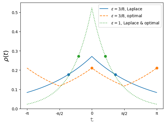
We use real numbers in $[-\pi,\pi)$ to denote users and results on a unit ring, and $\left<x,a\right>$ denotes $|x-a|$ . Figure 4 illustrates the optimal mechanism under geographic DP for $k=2$ . This mechanism uses noise that is a piece-wise composition of Laplace noises; we obtain a cost of 0.72 whereas Laplace noise gives a cost of 0.75. To find the optimal mechanism for the case of the ring, we solve the DILP $\mathcal{O}$ using a linear program solver and obtain the plot shown in Figure 4 with cost of 0.72. However, when the user sends Laplace noise, the server on receiving signal $z$ responds with two points $z+a_{1}$ and $z+a_{2}$ which maybe calculated by the following problem.

\displaystyle\min_{a_{1}\in[-\pi,\pi),a_{2}\in[-\pi,\pi)}\int_{-\pi}^{\pi}\min% \{\left<x,a_{1}\right>,\left<x,a_{2}\right>\}\rho(x)dx,

where $\rho(x)$ is a density function for the Laplace distribution,

A.3 Noise satisfying Monotone Hazard Rate property

Let $Y$ denote the random noise with density $g$ . We assume $Y$ is symmetric about the origin, and let $X=Y^{+}\cup\{0\}$ . Let $f$ denote the density function of $X$ (so that $f(x)=2g(x)$ for $x\geq 0$ ), and let $F(x)=\operatorname{\mathbb{P}}\left(X\geq x\right)$ . We assume that $\operatorname{\mathbb{E}}\left[X\right]=\frac{1}{\epsilon}$ .¹⁶¹⁶16This implies that a large $\epsilon$ is equivalent to the magnitude of noise being smaller and vice-versa. Although this distribution does not satisfy $\epsilon$ geographic differential privacy, this follows a similar trend w.r.t $\epsilon$ . We assume $f$ is continuously differentiable and log-concave. By [9], we have $F$ is also log-concave. Note that several natural distributions such as Exponential (Laplace noise) and Gaussian are log-concave.

We are interested in choosing $2K-1$ values $S=\{-a_{K-1},-a_{K-2},\ldots,-a_{1},0,a_{1},\ldots,a_{K-1}\}$ such that for a random draw $y\sim Y$ , the expected error in approximating $y$ by its closest point in $S$ is small. For $i=0,1,2,\ldots,K-1$ , we will choose $a_{i}=F^{-1}\left(1-\frac{i}{K}\right)$ . Let $\phi=\operatorname{\mathbb{E}}_{x\sim X}\left[\min\limits_{v\in S}|v-x|\right]$ . Note that the error of $Y$ with respect to $S$ is exactly $\phi$ .

Our main result is the following theorem:

Theorem 24.

$\phi=O\left(\frac{\log K}{K\epsilon}\right)$ .

Proof.

Let $G(z)=F^{-1}(z)$ for $z\in[0,1]$ . For upper bounding $\phi$ , we map each $x\sim X$ to the immediately smaller value in $S$ . If we draw $z\in[0,1]$ uniformly at random, the error is upper bounded as:

\phi\leq\int_{0}^{1}G(z)dz-\sum_{i=1}^{K}\frac{1}{K}G\left(\frac{i}{K}\right)% \leq\int_{0}^{1/K}\left(G(z)-G(1/K)\right)dz+\frac{1}{K}G(1/K).

Let $q=G(1/K).$ Then the above can be rewritten as: $\phi\leq\frac{q}{K}+\int_{q}^{\infty}F(x)dx$ . Next, it follows from [9] that if $F$ is log-concave, then so is $\int_{r}^{\infty}F(x)dx$ . This means the function $\ell(r)=\frac{\int_{r}^{\infty}F(x)dx}{F(r)}$ is non-increasing in $r$ . Therefore,

\int_{q}^{\infty}F(x)dx\leq F(q)\int_{0}^{\infty}F(x)dx=\frac{1}{K}% \operatorname{\mathbb{E}}\left[X\right]=\frac{1}{\epsilon K}.

Let $h(x)=-\log F(x)$ . Then, $h$ is convex and increasing. Further, $h(q)=\log K$ . Let $s=F^{-1}(1/e)$ so that $h(s)=1$ . Since $h(q)-h(s)\geq(q-s)h^{\prime}(s)$ , we have $q-s\leq\frac{\log K}{h^{\prime}(s)}$ . Further, $h(s)\leq sh^{\prime}(s)$ so that $\frac{1}{h^{\prime}(s)}\leq s$ . Since $F(s)=1/e$ and $\operatorname{\mathbb{E}}\left[X\right]=\frac{1}{\epsilon}\geq\int_{0}^{s}F(x)dx$ , we have $s\leq\frac{e}{\epsilon}$ . Therefore, $h^{\prime}(s)\geq 1/{e\epsilon}$ . Putting this together,

q\leq\frac{s}{\epsilon}+\frac{\log K}{h^{\prime}(s)}\leq\frac{e}{\epsilon}(1+% \log K)=O\left(\frac{\log K}{\epsilon}\right).

Therefore,

\phi\leq\frac{q}{K}+\int_{q}^{\infty}F(x)dx=O\left(\frac{\log K}{K\epsilon}% \right)+\frac{1}{K\epsilon}

completing the proof. $\hfill\blacktriangleleft$

A.4 Restricted and Unrestricted Setup of the Multi-Selection model

Recall the setup in Section 1 where the users and results belonged to different sets and $M$ with the definition of disutility in Definition 3. In section 1.1.4, we considered an alternate setup where the users and results belonged to the same set and the optimal result for an user $u$ was the result $u$ itself. In this section, we call these setups unrestricted and restricted respectively and define our “multi-selection” model separately for both these setups. Finally, we bound the cost function in the unrestricted setup by the cost function in the restricted setup in Theorem 25 thus, showing that it is sufficient to consider the cost function in the restricted setup.

Unrestricted setup.

Recall that results and users are located in sets ${M}$ and respectively and function $\text{OPT}:\real\rightarrow M$ maps every user to its optimal result(ad). Recall that the disutility of an user $u$ from a result $m$ is defined in Definition 3.

Restricted setup.

This setup is very similar to the setup described except the fact that users and results(ads) lie on the same set . Recall from Section 1.1.4, the disutility of an user $u\in\real$ from a result $a\in\real$ is given by $\mathfrak{h}(|u-a|)$ for some function $\mathfrak{h}(.)$ satisfying equations (2) and (3).

A.4.1 The space of server/user actions

Recall that the goal is to determine a mechanism that has the following ingredients:

1.

A set of signals $Z$ .
2.

The action of users, which involves choosing a signal from a distribution over signals. We use $P_{u}$ for $u\in\real$ to denote the distribution of the signals sent by user $u$ . This distribution is supported on $Z$ .
3.

The distribution over actions of the server, $Q_{s}$ when it receives $s\in Z$ . This distribution denoting the distribution of the result set returned by the server given signal $s$ may be supported on either ^k or $M^{k}$ , for the restricted setup and unrestricted setup respectively.

The optimal mechanism is computed by jointly optimizing over the tuple $(Z,\mathbf{P},\mathbf{Q})$ . And thus, we define the set of server responses by $\mathcal{Q}_{\text{unrestricted},Z}$ and $\mathcal{Q}_{\text{restricted},Z}$ for unrestricted and restricted setup respectively.

$\blacksquare$

$\mathcal{Q}_{\text{unrestricted},Z}:=\{\mathbf{Q}|\forall s\in Z,Q_{s}\text{% \leavevmode\nobreak\ is a distribution on $M^{k}$}\}$ .
$\blacksquare$

$\mathcal{Q}_{\text{restricted},Z}:=\{\mathbf{Q}|\forall s\in Z,Q_{s}\text{% \leavevmode\nobreak\ is a distribution on $\real{}^{k}$}\}$ .

In any feasible geographic DP mechanism, the user behavior should satisfy $\epsilon$ -geographic differential privacy: for any $u_{1},u_{2}\in\real$ , it should hold that $P_{u_{1}}(S)\leq P_{u_{2}}(S)e^{\epsilon|u_{1}-u_{2}|}$ where $S$ is any measurable subset of $Z$ . For any fixed response size $k$ , in order to maximize utility while ensuring the specified level of privacy, the goal is to minimize the disutility of the user from the result that the gives the user minimum disutility where the minimisation is the worst case user $u$ in .

A.4.2 Cost functions in both the setups

For the unrestricted and restricted setups, we define the cost functions ${f}_{\text{unrestricted}}^{\mathfrak{h}(.)}(\epsilon,k)$ and ${f}_{\text{unrestricted}}^{\mathfrak{h}(.)}(\epsilon,k)$ respectively below. Recall that $Z$ may denote any set.

	$\displaystyle{f}_{\text{unrestricted}}^{\mathfrak{h}(.)}(\epsilon,k)$	$\displaystyle:=\inf_{Z}\inf_{\begin{subarray}{c}\mathbf{P}\in\mathcal{P}^{(% \epsilon)}_{Z}\\ \mathbf{Q}\in\mathcal{Q}_{\text{unrestricted},Z}\end{subarray}}\sup_{u\in\real% }\mathop{\operatorname{\mathbb{E}}}\limits_{s\sim P_{u},\textbf{a}\sim Q_{s}}% \left[\min_{a\in\texttt{Set}(\textbf{a})}\left(\text{Dis-util}^{\mathfrak{h}(.% )}(u,a)\right)\right]$		(19)
	$\displaystyle{f}_{\text{restricted}}^{\mathfrak{h}(.)}(\epsilon,k)$	$\displaystyle:=\inf_{Z}\inf_{\begin{subarray}{c}\mathbf{P}\in\mathcal{P}^{(% \epsilon)}_{Z}\\ \mathbf{Q}\in\mathcal{Q}_{\text{restricted},Z}\end{subarray}}\sup_{u\in\real}% \mathop{\operatorname{\mathbb{E}}}\limits_{s\sim P_{u},\textbf{a}\sim Q_{s}}% \left[\min_{a\in\texttt{Set}(\textbf{a})}\mathfrak{h}\left(\|u-a\|\right)\right]% ,\text{ where }$		(20)

$\mathcal{P}^{(\epsilon)}_{Z}:=\{\mathbf{P}|\forall u\in\real,P_{u}\text{% \leavevmode\nobreak\ is a distribution on $Z$,}\text{\leavevmode\nobreak\ and % $\epsilon$-geographic differential privacy is}$ $\text{satisfied}\}$ .

We state a theorem upper bounding ${f}_{\text{unrestricted}}^{\mathfrak{h}(.)}(\epsilon,k)$ by ${f}_{\text{restricted}}^{\mathfrak{h}(.)}(\epsilon,k)$ .

Theorem 25.

For any $\mathfrak{h}(.)$ satisfying equation (2), we have ${f}_{\text{unrestricted}}^{\mathfrak{h}(.)}(\epsilon,k)\leq{f}_{\text{% restricted}}^{\mathfrak{h}(.)}(\epsilon,k)$ .

A detailed proof for the same is provided in [41, Appendix B.4.4] using the fact that $\text{Dis-util}^{\mathfrak{h}(.)}(u,\text{OPT}(u^{\prime}))\leq\mathfrak{h}(|u% -u^{\prime}|)$ .

Appendix B Server response for odd $𝒌$ when $\mathfrak{h}(.)$ is an identity function

We now show the optimal choice of $A$ to optimize cost function $\hat{f}(\epsilon,k)$ [in Equation (14)]. Specifically, we assume odd $k$ in this section. The solution for even $k$ (refer [41, Theorem C.3]) can be constructed using a similar induction where the base case for $k=2$ can be directly optimized. Assuming the symmetry of $A$ , let $A=\{-y_{b-1},\ldots-y_{1},0,y_{1},\ldots,y_{b-1}\}$ , where $y_{1},\ldots,y_{b-1}$ are positive numbers in increasing order. We will construct the set $y_{1},\ldots,y_{b-1}$ inductively. Let $x$ be a random variable drawn from Laplace distribution $\mathcal{L}_{\epsilon}(0)$ with parameter $\epsilon$ , and the goal is to minimize $D_{b}=\operatorname{\mathbb{E}}_{x\sim\mathcal{L}_{\epsilon}(0)}\left[\min% \limits_{a\in A}\mathfrak{h}(|x-a|)\right]$ . Since the density function of $\mathcal{L}_{\epsilon}(0)$ satisfies $\rho_{\mathcal{L}_{\epsilon}(0)}(x)=\rho_{\mathcal{L}_{\epsilon}(0)}(-x)$ , we have

D_{b}=\operatorname{\mathbb{E}}_{x\sim\mathcal{L}_{\epsilon}(0)}\left[\min_{a% \in A}\mathfrak{h}(|x-a|)\bigg{|}x>0\right],

i.e. the user has a positive private value. Under this conditioning, the variable $x$ is an exponential random variable of mean 1. In this case, the search result being used by the server will be one of $y_{0},y_{1}$ , …, $y_{b-1}$ . Clearly, $D_{1}=1$ . To compute $D_{b+1}$ , let $s=y_{1}$ . Then using the memorylessness property of exponential random variables, we get the recurrence

	$\displaystyle D_{b+1}$	$\displaystyle=\int_{t=0}^{s}\min\{\mathfrak{h}(t),\mathfrak{h}(s-t)\}e^{-t}dt+% e^{-s}D_{b}$
		$\displaystyle=\int_{t=0}^{s/2}\mathfrak{h}(t)e^{-t}dt+s\int_{t=s/2}^{s}e^{-t}% dt-\int_{t=s/2}^{s}\mathfrak{h}(t)e^{-t}dt+e^{-s}D_{b}.$

The optimal $D_{b+1}$ given $D_{b}$ can be computed by minimising over all $s\in\mathbb{R}$ . However, for the case where $\mathfrak{h}(.)$ is an identity function, we may give a closed form expression below.

	$\displaystyle D_{b+1}=$	$\displaystyle\int_{t=0}^{s/2}te^{-t}dt+s\int_{t=s/2}^{s}e^{-t}dt-\int_{t=s/2}^% {s}te^{-t}dt+e^{-s}D_{b}$
	$\displaystyle=$	$\displaystyle\left(1-(s/2)e^{-s/2}-e^{-s/2}\right)+s\left(e^{-s/2}-e^{-s}% \right)-$
		$\displaystyle\left((s/2)e^{-s/2}+e^{-s/2}-se^{-s}-e^{-s}\right)+e^{-s}D_{b}$
	$\displaystyle=$	$\displaystyle\left(1-e^{-s/2}\right)^{2}+\left(e^{-s/2}\right)^{2}D_{b}$

Setting $\gamma=e^{-s/2}$ , and minimizing by taking derivatives, we get $-2(1-\gamma)+2\gamma D_{b}=0$ which in turn gives $\gamma=\frac{1}{D_{b}+1}$ and $D_{b+1}=\frac{D_{b}}{D_{b}+1}$ . Plugging in the inductive hypothesis of $D_{b}=1/b$ , we get $D_{b+1}=1/(b+1)$ . Further, we get $s=2\ln(1+1/b)$ . Thus, by returning $k=2b-1$ results, the expected “cost of privacy” can be reduced by a factor of $b$ . To obtain the actual positions $y_{1},..,y_{b-1}$ we have to unroll the induction. For $i=1,\ldots,b-1$ , the position $y_{i}$ is given by:

y_{i}=y_{i-1}+2\ln(1+1/(b-i)).

[bib.bib1] [1] Mário S. Alvim, Konstantinos Chatzikokolakis, Catuscia Palamidessi, and Anna Pazii. Metric-based local differential privacy for statistical applications, 2018. arXiv:1805.01456.

[bib.bib2] [2] EJ Anderson. A new continuous model for job-shop scheduling. International journal of systems science, 12(12):1469–1475, 1981.

[bib.bib3] [3] E.J. Anderson and P. Nash. Linear Programming in Infinite-dimensional Spaces: Theory and Applications. A Wiley-Interscience publication. Wiley, 1987. URL: https://books.google.com/books?id=O2VRAAAAMAAJ.

[bib.bib4] [4] Miguel E Andrés, Nicolás E Bordenabe, Konstantinos Chatzikokolakis, and Catuscia Palamidessi. Geo-indistinguishability: Differential privacy for location-based systems. In Proceedings of the 2013 ACM SIGSAC conference on Computer & communications security, pages 901–914, 2013.

[bib.bib5] [5] Elliot Anshelevich and John Postl. Randomized social choice functions under metric preferences, 2016. arXiv:1512.07590.

[bib.bib6] [6] Apple. Learning with privacy at scale. Apple Machine Learning Journal, 1, 2017. URL: https://machinelearning.apple.com/2017/12/06/learning-with-privacy-at-scale.html.

[bib.bib7] [7] Brendan Avent, Yatharth Dubey, and Aleksandra Korolova. The power of the hybrid model for mean estimation. The 20th Privacy Enhancing Technologies Symposium (PETS), 2020.

[bib.bib8] [8] Brendan Avent, Aleksandra Korolova, David Zeber, Torgeir Hovden, and Benjamin Livshits. BLENDER: Enabling local search with a hybrid differential privacy model. In 26th USENIX Security Symposium (USENIX Security 17); Journal of Privacy and Confidentiality, 2019.

[bib.bib9] [9] M. Bagnoli and T. Bergstrom. Log-Concave Probability And Its Applications. Papers 89-23, Michigan - Center for Research on Economic & Social Theory, 1989. URL: https://ideas.repec.org/p/fth/michet/89-23.html.

[bib.bib10] [10] Raef Bassily, Albert Cheu, Shay Moran, Aleksandar Nikolov, Jonathan Ullman, and Steven Wu. Private query release assisted by public data. In International Conference on Machine Learning, pages 695–703. PMLR, 2020.

[bib.bib11] [11] Raef Bassily, Kobbi Nissim, Uri Stemmer, and Abhradeep Guha Thakurta. Practical locally private heavy hitters. Advances in Neural Information Processing Systems, 30, 2017.

[bib.bib12] [12] Amitabh Basu, Kipp Martin, and Christopher Thomas Ryan. Strong duality and sensitivity analysis in semi-infinite linear programming, 2015. arXiv:1510.07531.

[bib.bib13] [13] Björn Bebensee. Local differential privacy: a tutorial. arXiv preprint arXiv:1907.11908, 2019. arXiv:1907.11908.

[bib.bib14] [14] Amos Beimel, Aleksandra Korolova, Kobbi Nissim, Or Sheffet, and Uri Stemmer. The power of synergy in differential privacy: Combining a small curator with local randomizers. In Information-Theoretic Cryptography (ITC), 2020.

[bib.bib15] [15] R. Bellman. Dynamic Programming. Princeton Landmarks in Mathematics and Physics. Princeton University Press, 2010. URL: https://books.google.co.in/books?id=92aYDwAAQBAJ.

[bib.bib16] [16] Avrim Blum, Katrina Ligett, and Aaron Roth. A learning theory approach to noninteractive database privacy. Journal of the ACM (JACM), 60(2):1–25, 2013. doi:10.1145/2450142.2450148.

[bib.bib17] [17] Hai Brenner and Kobbi Nissim. Impossibility of differentially private universally optimal mechanisms. SIAM Journal on Computing, 43(5):1513–1540, 2014. doi:10.1137/110846671.

[bib.bib18] [18] Mark Bun, Jelani Nelson, and Uri Stemmer. Heavy hitters and the structure of local privacy. ACM Transactions on Algorithms (TALG), 15(4):1–40, 2019. doi:10.1145/3344722.

[bib.bib19] [19] James Burke. Duality in linear programming. https://sites.math.washington.edu//˜burke/crs/407/notes/section4.pdf. Accessed: 2010-09-30.

[bib.bib20] [20] Ioannis Caragiannis, Nisarg Shah, and Alexandros A. Voudouris. The metric distortion of multiwinner voting. Artificial Intelligence, 313:103802, 2022. doi:10.1016/j.artint.2022.103802.

[bib.bib21] [21] Rui Chen, Haoran Li, A Kai Qin, Shiva Prasad Kasiviswanathan, and Hongxia Jin. Private spatial data aggregation in the local setting. In 2016 IEEE 32nd International Conference on Data Engineering (ICDE), pages 289–300. IEEE, 2016. doi:10.1109/ICDE.2016.7498248.

[bib.bib22] [22] Albert Cheu, Adam Smith, Jonathan Ullman, David Zeber, and Maxim Zhilyaev. Distributed differential privacy via shuffling. In Advances in Cryptology–EUROCRYPT 2019: 38th Annual International Conference on the Theory and Applications of Cryptographic Techniques, Darmstadt, Germany, May 19–23, 2019, Proceedings, Part I 38, pages 375–403. Springer, 2019. doi:10.1007/978-3-030-17653-2_13.

[bib.bib23] [23] Ilaria Chillotti, Marc Joye, and Pascal Paillier. New challenges for fully homomorphic encryption. In Privacy Preserving Machine Learning - PriML and PPML Joint Edition Workshop, NeurIPS 2020, December 2020. URL: https://neurips.cc/virtual/2020/19640.

[bib.bib24] [24] B. Chor, O. Goldreich, E. Kushilevitz, and M. Sudan. Private information retrieval. In Proceedings of the 36th Annual Symposium on Foundations of Computer Science, FOCS ’95, page 41, USA, 1995. IEEE Computer Society.

[bib.bib25] [25] Bolin Ding, Janardhan Kulkarni, and Sergey Yekhanin. Collecting telemetry data privately. Advances in Neural Information Processing Systems, 30, 2017.

[bib.bib26] [26] John C. Duchi, Michael I. Jordan, and Martin J. Wainwright. Local privacy and statistical minimax rates. In 2013 IEEE 54th Annual Symposium on Foundations of Computer Science, pages 429–438, 2013. doi:10.1109/FOCS.2013.53.

[bib.bib27] [27] Cynthia Dwork, Frank McSherry, Kobbi Nissim, and Adam Smith. Calibrating noise to sensitivity in private data analysis. In Theory of Cryptography: Third Theory of Cryptography Conference, TCC 2006, New York, NY, USA, March 4-7, 2006. Proceedings 3, pages 265–284. Springer, 2006. doi:10.1007/11681878_14.

[bib.bib28] [28] Cynthia Dwork and Aaron Roth. The algorithmic foundations of differential privacy. Foundations and Trends® in Theoretical Computer Science, 9(3–4):211–407, 2014. doi:10.1561/0400000042.

[bib.bib29] [29] Cynthia Dwork, Aaron Roth, et al. The algorithmic foundations of differential privacy. Foundations and Trends® in Theoretical Computer Science, 9(3–4):211–407, 2014. doi:10.1561/0400000042.

[bib.bib30] [30] Úlfar Erlingsson, Vitaly Feldman, Ilya Mironov, Ananth Raghunathan, Kunal Talwar, and Abhradeep Thakurta. Amplification by shuffling: From local to central differential privacy via anonymity. In Proceedings of the Thirtieth Annual ACM-SIAM Symposium on Discrete Algorithms, pages 2468–2479. SIAM, 2019. doi:10.1137/1.9781611975482.151.

[bib.bib31] [31] Úlfar Erlingsson, Vasyl Pihur, and Aleksandra Korolova. RAPPOR: Randomized aggregatable privacy-preserving ordinal response. In Proceedings of the 2014 ACM SIGSAC Conference on Computer and Communications Security, CCS ’14, pages 1054–1067, New York, NY, USA, 2014. ACM. doi:10.1145/2660267.2660348.

[bib.bib32] [32] Lawrence C Evans. An introduction to mathematical optimal control theory version 0.2. Lecture notes available at http://math. berkeley. edu/˜ evans/control. course. pdf, 1983.

[bib.bib33] [33] Vitaly Feldman, Audra McMillan, and Kunal Talwar. Hiding among the clones: A simple and nearly optimal analysis of privacy amplification by shuffling. In 2021 IEEE 62nd Annual Symposium on Foundations of Computer Science (FOCS), pages 954–964. IEEE, 2022.

[bib.bib34] [34] Natasha Fernandes, Annabelle McIver, and Carroll Morgan. The laplace mechanism has optimal utility for differential privacy over continuous queries. In 2021 36th Annual ACM/IEEE Symposium on Logic in Computer Science (LICS), pages 1–12. IEEE, 2021. doi:10.1109/LICS52264.2021.9470718.

[bib.bib35] [35] K. O. Friedrichs. The identity of weak and strong extensions of differential operators. Transactions of the American Mathematical Society, 55(1):132–151, 1944. URL: http://www.jstor.org/stable/1990143.

[bib.bib36] [36] Kurt Otto Friedrichs. The identity of weak and strong extensions of differential operators. Transactions of the American Mathematical Society, 55(1):132–151, 1944.

[bib.bib37] [37] Quan Geng and Pramod Viswanath. The optimal noise-adding mechanism in differential privacy. IEEE Transactions on Information Theory, 62(2):925–951, 2015. doi:10.1109/TIT.2015.2504967.

[bib.bib38] [38] Robin C. Geyer, Tassilo J. Klein, and Moin Nabi. Differentially private federated learning: A client level perspective. arXiv preprint arXiv:1712.07557, 2017.

[bib.bib39] [39] Arpita Ghosh, Tim Roughgarden, and Mukund Sundararajan. Universally utility-maximizing privacy mechanisms. SIAM Journal on Computing, 41(6):1673–1693, 2012. doi:10.1137/09076828X.

[bib.bib40] [40] Vasilis Gkatzelis, Daniel Halpern, and Nisarg Shah. Resolving the optimal metric distortion conjecture. In 2020 IEEE 61st Annual Symposium on Foundations of Computer Science (FOCS), pages 1427–1438. IEEE, 2020. doi:10.1109/FOCS46700.2020.00134.

[bib.bib41] [41] Ashish Goel, Zhihao Jiang, Aleksandra Korolova, Kamesh Munagala, and Sahasrajit Sarmasarkar. Differential privacy with multiple selections, 2024. doi:10.48550/arXiv.2407.14641.

[bib.bib42] [42] Saikat Guha, Bin Cheng, and Paul Francis. Privad: Practical privacy in online advertising. In USENIX conference on Networked systems design and implementation, pages 169–182, 2011.

[bib.bib43] [43] Mangesh Gupte and Mukund Sundararajan. Universally optimal privacy mechanisms for minimax agents. In Proceedings of the twenty-ninth ACM SIGMOD-SIGACT-SIGART symposium on Principles of database systems, pages 135–146, 2010. doi:10.1145/1807085.1807105.

[bib.bib44] [44] F. Maxwell Harper and Joseph A. Konstan. The movielens datasets: History and context. ACM Trans. Interact. Intell. Syst., 5(4), December 2015. doi:10.1145/2827872.

[bib.bib45] [45] Alexandra Henzinger, Emma Dauterman, Henry Corrigan-Gibbs, and Nickolai Zeldovich. Private web search with Tiptoe. In 29th ACM Symposium on Operating Systems Principles (SOSP), Koblenz, Germany, October 2023.

[bib.bib46] [46] Peter Kairouz, Sewoong Oh, and Pramod Viswanath. Extremal mechanisms for local differential privacy. Advances in neural information processing systems, 27, 2014.

[bib.bib47] [47] Shiva Prasad Kasiviswanathan, Homin K Lee, Kobbi Nissim, Sofya Raskhodnikova, and Adam Smith. What can we learn privately? SIAM Journal on Computing, 40(3):793–826, 2011. doi:10.1137/090756090.

[bib.bib48] [48] Fatih Erdem Kizilkaya and David Kempe. Plurality veto: A simple voting rule achieving optimal metric distortion. arXiv preprint arXiv:2206.07098, 2022. doi:10.48550/arXiv.2206.07098.

[bib.bib49] [49] Fragkiskos Koufogiannis, Shuo Han, and George J Pappas. Optimality of the laplace mechanism in differential privacy. arXiv preprint arXiv:1504.00065, 2015. arXiv:1504.00065.

[bib.bib50] [50] Jingcheng Liu and Kunal Talwar. Private selection from private candidates. In Proceedings of the 51st Annual ACM SIGACT Symposium on Theory of Computing, pages 298–309, 2019. doi:10.1145/3313276.3316377.

[bib.bib51] [51] Chiara Marcolla, Victor Sucasas, Marc Manzano, Riccardo Bassoli, Frank H.P. Fitzek, and Najwa Aaraj. Survey on fully homomorphic encryption, theory, and applications. Cryptology ePrint Archive, Paper 2022/1602, 2022. doi:10.1109/JPROC.2022.3205665.

[bib.bib52] [52] Frank McSherry and Kunal Talwar. Mechanism design via differential privacy. In 48th Annual IEEE Symposium on Foundations of Computer Science (FOCS’07), pages 94–103. IEEE, 2007. doi:10.1109/FOCS.2007.41.

[bib.bib53] [53] Nicolas Papernot, Shuang Song, Ilya Mironov, Ananth Raghunathan, Kunal Talwar, and Úlfar Erlingsson. Scalable private learning with pate, 2018. arXiv:1802.08908.

[bib.bib54] [54] Malcolm C. Pullan. An algorithm for a class of continuous linear programs. SIAM Journal on Control and Optimization, 31(6):1558–1577, 1993. doi:10.1137/0331073.

[bib.bib55] [55] Apple Machine Learning Research. Learning with privacy at scale: Differential privacy for aggregate trend analysis. https://machinelearning.apple.com/research/differential-privacy-aggregate-trends, 2023. Accessed: 28th May 2025.

[bib.bib56] [56] W. Rudin. Principles of Mathematical Analysis. International series in pure and applied mathematics. McGraw-Hill, 1976. URL: https://books.google.com/books?id=kwqzPAAACAAJ.

[bib.bib57] [57] Sahasrajit Sarmasarkar, Zhihao Jiang, Ashish Goel, Aleksandra Korolova, and Kamesh Munagala. Multi-selection for recommendation systems, 2025. arXiv:2504.07403.

[bib.bib58] [58] Vincent Toubiana, Arvind Narayanan, Dan Boneh, Helen Nissenbaum, and Solon Barocas. Adnostic: Privacy preserving targeted advertising. NDSS, 2010.

[bib.bib59] [59] N.T. Vinh, D.S. Kim, N.N. Tam, and N.D. Yen. Duality gap function in infinite dimensional linear programming. Journal of Mathematical Analysis and Applications, 437(1):1–15, 2016. doi:10.1016/j.jmaa.2015.12.043.

[bib.bib60] [60] Tianhao Wang, Jeremiah Blocki, Ninghui Li, and Somesh Jha. Locally differentially private protocols for frequency estimation. In 26th USENIX Security Symposium (USENIX Security 17), pages 729–745, 2017. URL: https://www.usenix.org/conference/usenixsecurity17/technical-sessions/presentation/wang-tianhao.

Differential Privacy Under Multiple Selections

Abstract

Keywords and phrases:

Funding:

Copyright and License:

2012 ACM Subject Classification:

Related Version:

Acknowledgements:

DOI:

Event:

Editors:

Series and Publisher:

1 Introduction

1.1 System Architecture and Definitions

1.1.1 Privacy

Definition 1 (adapted from [26, 49]).

Definition 2 (adapted from [49]).

1.1.2 “Multi-Selection” Architecture

1.1.3 The disutility model: Measuring the cost of privacy

Definition 3.

Example 4.

1.1.4 Restricting users and results to the same set

1.1.5 Definition of the cost function in the simplified setup

1.2 Our results and key technical contributions

Theorem 5 (corresponds to Theorem 19 and Theorem C.3 in [41]).

1.3 Related Work

1.3.1 Differential Privacy

1.3.2 Multi-Selection

1.3.3 Optimal DP mechanisms

1.3.4 Homomorphic encryption

1.3.5 Related work on duality theory for infinite dimensional LPs

2 Characterizing the Optimal Mechanism: Proof Sketch of Theorem 5

Definition 6.

2.1 Restricting the signal set 𝒁 to ℝ𝒌

Example 7.

Theorem 8 (detailed proof in Appendix C.1 of [41]).

Proof Sketch.

2.2 Differential integral linear programs to represent 𝒇⁢(ϵ,𝒌) and a weak duality result

2.2.1 Construction of DILP 𝓞 to represent cost function 𝒇⁢(ϵ,𝒌)

Definition 9.

Definition 10.

Lemma 11.

Lemma 12.

Lemma 13.

Proof of Lemma 11.

2.2.2 Dual DILP 𝓔 and statement of weak duality theorem

Theorem 14.

2.3 Dual fitting to show the optimality of Laplace noise addition

2.3.1 Bounding cost function 𝒇⁢(ϵ,𝒌) by the cost of Laplace noise adding mechanism

Definition 15.

Lemma 16 (detailed proof in Appendix C.3 of [41]).

Proof Sketch.

2.3.2 Obtaining a feasible solution to DILP 𝓔

Lemma 17 (Proof in Appendix C.4.2 of [41]).

Intuitive explanation.

Lemma 18 (detailed proof in Appendix C.4.2 of [41]).

Proof Sketch.

Theorem 19.

Proof.

2.4 Server response given the user sends Laplace Noise

3 Conclusion

References

Appendix A Further extensions

A.1 A generalization of Geographic differential privacy

Assumption 20.

Definition 21 (alternate definition of geo-DP).

Theorem 22.

Proof.

Lemma 23.

A.2 Calculation of optimal mechanism on a ring for the case of 𝒌=𝟐

A.3 Noise satisfying Monotone Hazard Rate property

Theorem 24.

Proof.

A.4 Restricted and Unrestricted Setup of the Multi-Selection model

Unrestricted setup.

Restricted setup.

A.4.1 The space of server/user actions

A.4.2 Cost functions in both the setups

Theorem 25.

Appendix B Server response for odd 𝒌 when 𝖍(.) is an identity function

2.1 Restricting the signal set $𝒁$ to $\mathbb{R}^{k}$

2.2 Differential integral linear programs to represent $f(\epsilon,k)$ and a weak duality result

2.2.1 Construction of DILP $\mathcal{O}$ to represent cost function $f(\epsilon,k)$

2.2.2 Dual DILP $\mathcal{E}$ and statement of weak duality theorem

2.3.1 Bounding cost function $f(\epsilon,k)$ by the cost of Laplace noise adding mechanism

2.3.2 Obtaining a feasible solution to DILP $\mathcal{E}$

A.2 Calculation of optimal mechanism on a ring for the case of $k=2$

Appendix B Server response for odd $𝒌$ when $\mathfrak{h}(.)$ is an identity function