Brief Announcement: The Shortest Temporal Exploration Problem

Abstract
A temporal graph is a graph for which the edge set can change from one time step to the next. This paper considers undirected temporal graphs defined over time steps and connected at each time step. We study the Shortest Temporal Exploration Problem (STEXP) that, given the evolution of the graph, asks for a temporal walk that starts at a given vertex, moves over at most one edge at each time step, visits all the vertices, takes at most time steps and traverses the smallest number of edges. We prove that every constantly connected temporal graph with vertices can be explored with edges traversed if is time steps. This result improves the upper bound of edges when is . Moreover, we study the case where the graph has a diameter bounded by a parameter at each time step and we prove that there exists an exploration which takes time steps and traverses edges. Finally, the case where the underlying graph is a cycle is studied and tight linear bounds are provided on the number of edges traversed in the worst-case.
Keywords and phrases:
Graph Theory, Temporal Graph, Temporal Graph ExplorationCopyright and License:
2012 ACM Subject Classification:
Mathematics of computing Graph theoryFunding:
This work was Supported by the French ANR, project ANR-22-CE48-0001 (TEMPOGRAL).Editors:
Kitty Meeks and Christian ScheidelerSeries and Publisher:
1 Introduction
Many real-life networks are not static objects because their connections may vary over time (e.g. transportation, communication, social interactions,…). A tool to modelize and study these networks is temporal graphs whose edge set changes over time. More formally, a temporal graph of lifetime may be defined as a sequence of undirected graphs called snapshots.
The adaptation of path-related problems from static graphs to temporal graphs raises several questions: mainly, the notion of path itself, and the optimization criteria to use. In a static graph, a set of edges connecting two vertices and is called a path between and , but in a temporal graph the equivalent is a journey from to which is a sequence of edges successive in time from to . It follows that, in temporal graphs, at least three criteria may be minimized when considering journeys: the length (the number of edges), the arrival time and the duration (the difference between the arrival time and the starting time of the agent).
An extensive study of these criteria in temporal graphs can be found in the article of Bui-Xuan et al.[4].
A well studied path-related problem in temporal graphs is the exploration problem introduced by Michail and Spirakis[3] which aims at finding a journey that visits all the vertices starting from a given vertex. They make the assumption that the graph is connected at each time step and that the agent already knows the evolution of the graph because it guarantees that an exploration exists if the lifetime is greater than where is the vertex set.
Most following papers studied the Temporal Exploration Problem (TEXP) which, given the evolution of the graph, starts at a given vertex and aims at minimizing the arrival time under the assumption that the graph is constantly connected [1]. We denote the Shortest Temporal Exploration Problem (STEXP) the Temporal Exploration Problem which, under the same hypothesis, aims at minimizing the number of edges traversed. The static graph whose edge set is the union of the edge sets of each snapshot is denoted the underlying graph and the total number of vertices is denoted by .
To the best of our knowledge no specific study exists on the STEXP.
In this brief annoucement the proofs are omitted because of the limited number of pages. A complete version with proofs can be found online.
2 Preliminaries
Definition 1 (Temporal graph).
A temporal graph with a vertex set and a lifetime is a sequence of static graphs where is called the snapshot at the time step .The underlying graph of is with the union of the edge sets of all the snapshot of .
In the rest of the paper, if no ambiguity arises, we will note the lifetime by and the vertex set by . We restrict our attention to always-connected graph. Moreover, when talking about journeys, we often refer to an agent that is supposed to traverse the edges of the journey.
Definition 2 (Path).
Let be a temporal graph. A path between the vertices and is a set of edges all belonging to the same snapshot and connecting and .
We highlight the fact that a path is associated to exactly one snapshot.
Definition 3 (Journey).
Let be a temporal graph. A journey from to is a sequence of edges of increasing time steps (not necessarily consecutive), , where , and . So an agent can go from to by traversing the edges of the sequence at the time step indicated.
There exist two types of journeys:
-
the non-strict journeys where the agent can traverse several edges per time step.
-
the strict journeys where the agent can traverse at most one edge per time step, i.e. .
Since constantly connected temporal graphs are studied, if non-strict journeys were allowed, there would be an exploration in time step with at most edge traversals. So only strict journeys are considered which means that at each time step the agent can either stay on a vertex or traverse an edge.
Definition 4 (Journey parameters).
Let be a temporal graph and the journey in .
-
Length
The length of is the number of edges of the journey, i.e. . -
Arrival time
The arrival time is the time step where the agent traverses the last edge that is . -
Duration
The duration is the number of time steps of the journey which is .
Definition 5 (Shortest Temporal Exploration Problem (STEXP)).
Given a temporal graph with a lifetime and a starting vertex , STEXP asks for a journey in starting on that visits all the vertices of the graph and has a minimum length.
In the rest of the paper we consider that is a constantly connected tempoal graph i.e. every snapshot is connected and is the starting vertex for the exploration. The notation is used for a journey from to in whose length is less than or equal to . Similarly, for a snapshot of we note a path connecting and with a number of edges less than or equal to in .
Lemma 6 (Reachability[3]).
Let be a temporal graph of lifetime and a pair of vertices. Then there is a strict journey from u to v starting at t, whose duration is at most .
This lemma implies the following result: considering any temporal graph , there is an exploration with an arrival time (and length) inferior or equal to .
3 The STEXP in the general case
Recall that our assumption is that each snapshot is connected and the agent already knows the evolution of the graph.
Let be a pair of vertices and . A sufficient condition for the existence of a journey of at most edges from to is first given.
Lemma 7.
Let be a temporal graph of vertices (not necessarily connected at each time steps) and such that , the lifetime of the graph is .
Let be two distinct vertices of , such that there exist distinct paths (i.e on distinct snapshots) with a number of edges less than or equal to connecting and , each of these paths is associated with exactly one time step. Then there exists a journey in using only these time steps.
This lemma links the existence of paths of bounded lengths to the existence of one journey of bounded length between two vertices. With this lemma we can create a journey which is a concatenation of journeys of at most edges such that each one visits a different vertex of .
Lemma 8.
Let be a temporal graph with a subset of vertices. Then there exists a journey visiting vertices of in timesteps with edge traversals.
The idea of the proof is that, given the set of unvisited vertices and a time-window of size , for every integer we can create a subset of denoted with the following property: for every vertex of , there is a vertex of such that there is a journey . By Lemma 7, we have that for any subset and any integer , is in the time-window of size . So, given and , we create a journey that is a concatenation of shorter journeys (each traversing edges), each visiting a vertex of that belongs to a set (each time the agent traverses one of these journeys with edges, the set is updated).
Theorem 9.
Let be a temporal graph with a lifetime which is . Then there exists an exploration of traversing edges in time steps.
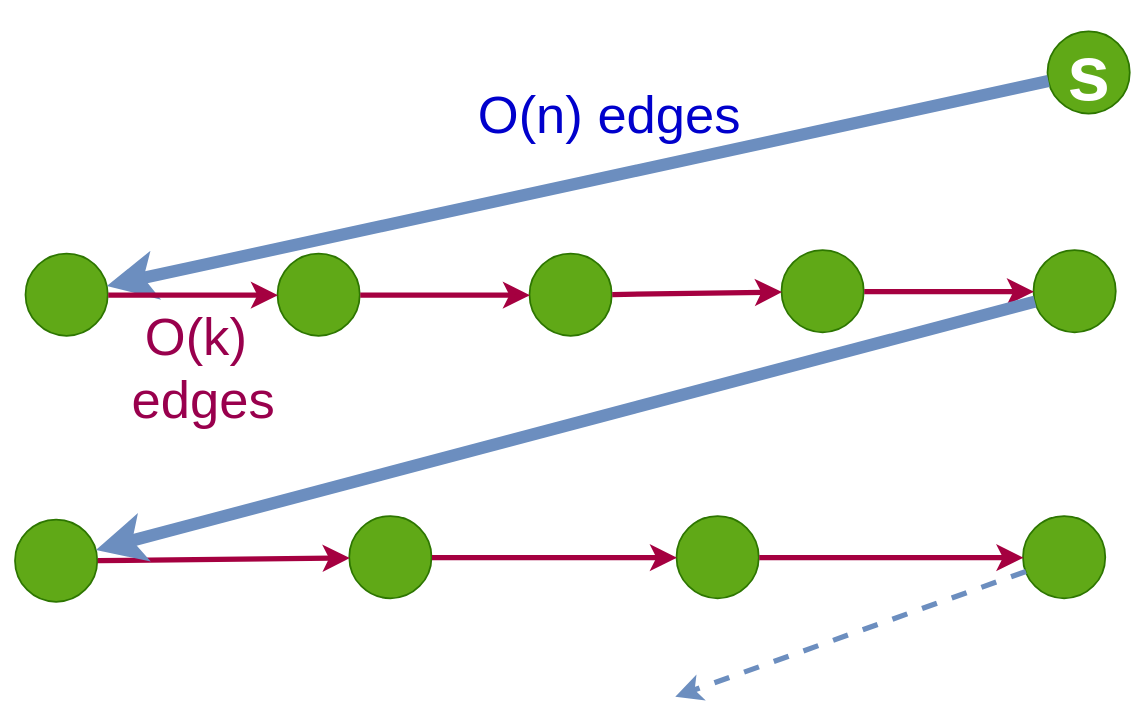
The theorem 9 is a corollary of Lemma 8 because we create an exploration in edge traversals with the following method. Let be the set of unvisited vertices and be the vertex on which the agent is present at the current time step. Recall that the agent can go to any vertex in time steps and by traversing at most edges by Lemma 6 so with this type of journey the agent goes to the starting vertex of a journey such as defined in the Lemma 8 that visits unvisited vertices. After this journey we update the set of unvisited vertices and reiterate the method until the agent visits all the vertices.
This concatenation of journeys forms the exploration such as presented in figure 1.
4 The case of bounded-diameter temporal graphs
Theorem 10.
Let be a temporal graph of vertices and an integer, the lifetime of the graph is . If , the snapshot has a diameter less than or equal to , then there exists an exploration of traversing less than edges.
The idea of the proof is that we can construct an exploration that visits all the vertices in an arbitrary order starting from . We visit an unvisited vertex every time steps with at most edge traversals because by assumption the distance between every pair of vertices is at most every time step. So, by Lemma 7, in a time-window of size , there is a journey traversing edges from the vertex on which the agent is present to the unvisited vertex. We repeat this method times to visit all the vertices of the temporal graph.
Erlebach et al.[1] have presented a family of temporal graphs such that each snapshot has a diameter and all explorations take time steps with edges traversed. We have proven that, for each temporal graph with , there is an exploration in time steps and edges traversed if each snapshot of has a bounded diameter. Hence our bounds are tight.
5 The case of the cycle as the underlying graph
In this section the following notations are used: is a temporal cycle which is a temporal graph whose underlying graph is a cycle, denoted .
Lemma 11.
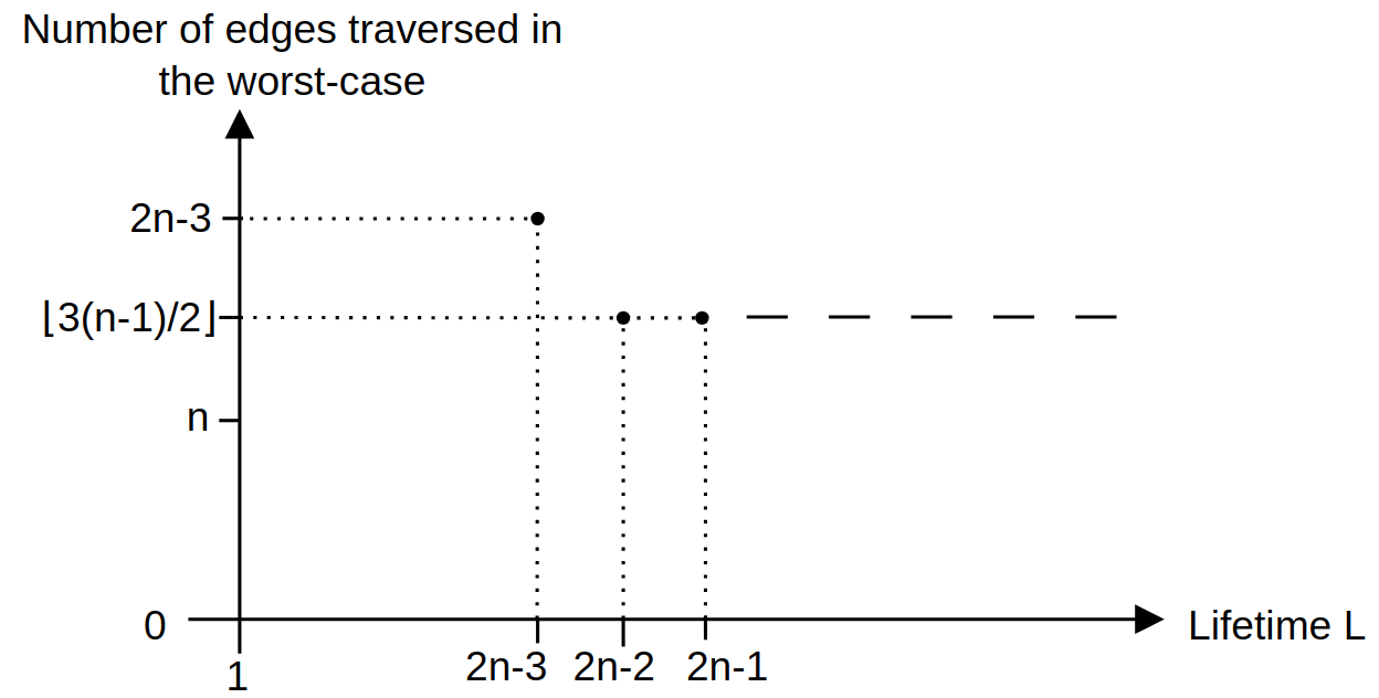
Let be a temporal cycle with a lifetime . In the worst-case scenario, the number of edges traversed for an exploration of is exactly edges.
Lemma 12.
For every integer , there exists a temporal cycle with vertices and a lifetime such that there is only one possible exploration and this exploration traverses exactly edges.
An overview of the results described by lemmas 11 and 12 is presented in figure 2. Since Ilcinkas et al.[2] proved that there is always an exploration if and only if , we start the value of the lifetime at in figure 2. So the bounds are tight for the number of edges traversed in STEXP.
References
- [1] Thomas Erlebach, Michael Hoffmann, and Frank Kammer. On temporal graph exploration. Journal of Computer and System Sciences, 119:1–18, 2021. doi:10.1016/J.JCSS.2021.01.005.
- [2] David Ilcinkas and Ahmed Mouhamadou Wade. Exploration of the t-interval-connected dynamic graphs: the case of the ring. In International Colloquium on Structural Information and Communication Complexity, pages 13–23. Springer, 2013. doi:10.1007/978-3-319-03578-9_2.
- [3] Othon Michail and Paul G Spirakis. Traveling salesman problems in temporal graphs. Theoretical Computer Science, 634:1–23, 2016. doi:10.1016/J.TCS.2016.04.006.
- [4] B Bui Xuan, Afonso Ferreira, and Aubin Jarry. Computing shortest, fastest, and foremost journeys in dynamic networks. International Journal of Foundations of Computer Science, 14(02):267–285, 2003. doi:10.1142/S0129054103001728.