Branch Prediction Analysis of Morris-Pratt and Knuth-Morris-Pratt Algorithms

Nicaud, Cyril; Pivoteau, Carine; Vialette, Stéphane

doi:10.4230/LIPIcs.CPM.2025.8

Branch Prediction Analysis of Morris-Pratt and Knuth-Morris-Pratt Algorithms

Cyril Nicaud

Univ Gustave Eiffel, CNRS, LIGM, F-77454 Marne-la-Vallée, France Carine Pivoteau Univ Gustave Eiffel, CNRS, LIGM, F-77454 Marne-la-Vallée, France Stéphane Vialette

Univ Gustave Eiffel, CNRS, LIGM, F-77454 Marne-la-Vallée, France

Abstract

We investigate the classical Morris-Pratt and Knuth-Morris-Pratt pattern matching algorithms from the perspective of computer architecture, focusing on the effects of incorporating a simple branch prediction mechanism into the computational model. Assuming a fixed pattern and a random text, we derive precise estimates for the number of branch mispredictions incurred by these algorithms when using local predictors. Our analysis relies on tools from automata theory and Markov chains, offering a theoretical framework that can be extended to other text processing algorithms and more sophisticated branch prediction strategies.

Keywords and phrases:

Pattern matching, branch prediction, transducers, average case complexity, Markov chains

Copyright and License:

2012 ACM Subject Classification:

Theory of computation

\rightarrow

Design and analysis of algorithms

DOI:

10.4230/LIPIcs.CPM.2025.8

Event:

36th Annual Symposium on Combinatorial Pattern Matching (CPM 2025)

Editors:

Paola Bonizzoni and Veli Mäkinen

Series and Publisher:

Leibniz International Proceedings in Informatics, Schloss Dagstuhl – Leibniz-Zentrum für Informatik

1 Introduction

Pipelining is a fundamental technique employed in modern processors to improve performance by executing multiple instructions in parallel, rather than sequentially. Instructions execution is divided into distinct stages, enabling the simultaneous processing of multiple instructions, much like an assembly line in a factory. Today, pipelining is ubiquitous, even in low-cost processors priced under a dollar. We refer the reader to the textbook reference [6] for more details on this important architectural feature.

The sequential execution model assumes that each instruction completes before the next one begins; however, this assumption does not hold in a pipelined processor. Specific conditions, known as hazards, may prevent the next instruction in the pipeline from executing during its designated clock cycle. Hazards introduce delays that undermine the performance benefits of pipelining and may stall the pipeline, thus reducing the theoretical speedup:

$\blacksquare$

Structural hazards occur when resource conflicts arise, preventing the hardware from supporting all possible combinations of instructions during simultaneous executions.
$\blacksquare$

Control hazards arise from the pipelining of jumps and other instructions that modify the order in which instructions are processed, by updating the Program Counter (PC).
$\blacksquare$

Data hazards occur when an instruction depends on the result of a previous instruction, and this dependency is exposed by the overlap of instructions in the pipeline.

To minimize stalls due to control hazards and improve execution efficiency, modern computer architectures incorporate branch predictors. A branch predictor is a digital circuit that anticipates the outcome of a branch (e.g., an if–then–else structure) before it is determined.

Two-way branching is typically implemented using a conditional jump instruction, which can either be taken, updating the Program Counter to the target address specified by the jump instruction and redirecting the execution path to a different location in memory, or not taken, allowing execution to continue sequentially. The outcome of a conditional jump remains unknown until the condition is evaluated and the instruction reaches the actual execution stage in the pipeline. Without branch prediction, the processor would be forced to wait until the conditional jump instruction reaches this stage before the next instruction can enter the first stage in the pipeline. The branch predictor aims to reduce this delay by predicting whether the conditional jump is likely to be taken or not. The instruction corresponding to the predicted branch is then fetched and speculatively executed. If the prediction is later found to be incorrect (i.e., a misprediction occurs), the speculatively executed or partially executed instructions are discarded, and the pipeline is flushed and restarted with the correct branch, incurring a small delay.

The effectiveness of a branch prediction scheme depends on both its accuracy and the frequency of conditional branches. Static branch prediction is the simplest technique, as it does not depend on the code execution history and, therefore, cannot adapt to program behavior. In contrast, dynamic branch prediction takes advantage of runtime information (specifically, branch execution history) to determine whether branches were taken or not, allowing it to make more informed predictions about future branches.

A vast body of research is dedicated to dynamic branch prediction schemes. At the highest level, branch predictors are classified into two categories: global and local. A global branch predictor does not maintain separate history records for individual conditional jumps. Instead, it relies on a shared history of all jumps, allowing it to capture their correlations and improve prediction accuracy. In contrast, a local branch predictor maintains an independent history buffer for each conditional jump, enabling predictions based solely on the behavior of that specific branch. Since the 2000s, modern processors typically employ a combination of local and global branch prediction techniques, often incorporating even more sophisticated designs. For a deeper exploration of this topic, see [10], and for a comprehensive discussion of modern computer architecture, refer to [6].

In this study, we focus on local branch predictors implemented with saturated counters. A 1-bit saturating counter (essentially a flip-flop) records the most recent branch outcome. Although this is the simplest form of dynamic branch prediction, it offers limited accuracy. A 2-bit saturating counter (see Figure 1), by contrast, operates as a state machine with four possible states: Strongly not taken ( $\underline{\nu}$ ), Weakly not taken ( $\nu$ ), Weakly taken ( $\tau$ ), and Strongly taken ( $\underline{\tau}$ ). When the 2-bit saturated branch predictor is in the Strongly not taken or Weakly not taken state, it predicts that the branch will not be taken and execution will proceed sequentially. Conversely, when the predictor is in the Strongly taken or Weakly taken state, it predicts that the branch will be taken, meaning execution will jump to the target address. Each time a branch is evaluated, the corresponding state machine updates its state. If the branch is not taken, the state shifts toward Strongly not taken; if taken, it moves toward Strongly taken. A misprediction (corresponding to a bold edge in Figure 1) occurs when:

$\blacksquare$

a branch is not taken, while the predictor is in either of the Taken states ( $\tau$ or $\underline{\tau}$ );
$\blacksquare$

a branch is taken, while the predictor is in either of the Not Taken states ( $\nu$ or $\underline{\nu}$ ).

This mechanism gives the 2-bit saturating counter an advantage over the simpler 1-bit scheme: a branch must deviate twice from its usual behavior (i.e. a Strongly state) before the prediction changes, reducing the likelihood of mispredictions.

Figure 1: The 2-bit saturated predictor consists of four states:

\underline{\nu}

and

\nu

predict that the branch will not be taken, while

\tau

and

\underline{\tau}

predict that it will. The predictor updates at each condition evaluation, transitioning via

T

when the branch is taken (i.e., the condition is true) and via

N

when it is not. Bold edges indicate mispredictions.

This paper presents an initial theoretical investigation into the techniques and results related to the analysis of pattern matching algorithms within computational models augmented by branch prediction mechanisms. In particular, we study the classical Morris-Pratt (MP) and Knuth-Morris-Pratt (KMP) algorithms [11, 7] in such models, with a primary focus on quantifying branch mispredictions under random text inputs. Over the past two decades, research in this area has evolved from experimental studies on sorting algorithms and fundamental data structures [2] to theoretical analyses of misprediction behavior in Java’s dual-pivot Quicksort [9], as well as the design of skewed variants of classical algorithms (e.g., binary search, exponentiation by squaring) aimed at improving branch prediction efficiency [1]. These studies have largely focused on local predictors – particularly 2-bit saturating counters (see Figure 1) – which also serve as the basis for the models considered in this work.

2 Algorithms and their encoding using transducers

Throughout the article, indices start at $0$ : if $u$ is a word of length $|u|=n$ over the alphabet $A$ , we represent it as $u=u_{0}\dots u_{n-1}$ , where each $u_{i}$ is a letter of $u$ . We also use $u[i]$ to denote the letter $u_{i}$ . If $u=xyz$ where $x$ , $y$ and $z$ are words, then $x$ is a prefix of $u$ , $y$ is a factor and $z$ is a suffix. A prefix (resp. suffix) of $u$ is strict if it differs from $u$ . For any $i\in\{0,\dots,n\}$ , we denote by $\operatorname{Pref}(u,i)$ the prefix of $u$ of length $i$ . A (strict) border of $u$ is a word $v$ that is both a (strict) prefix and a (strict) suffix of $u$ .

Algorithms MP and KMP

The Morris-Pratt (MP) and Knuth-Morris-Pratt (KMP) algorithms are textbook solutions to the pattern matching problem [4, 5, 3]. Both rely on precomputing a failure function, which helps identify candidate positions for the pattern $X$ in the text $W$ . The general approach involves scanning $W$ from left to right, one letter at a time. Before moving to the next letter in $W$ , the algorithm determines the longest prefix of $X$ that is also a suffix of the discovered prefix of $W$ . The failure function allows this computation to be performed efficiently.

The function $\textrm{mp}_{X}$ maps each prefix of $X$ to its longest strict border, with the convention that $\textrm{mp}_{X}(\varepsilon)=\bot$ . The function $\textrm{kmp}_{X}$ is a refinement of $\textrm{mp}_{X}$ defined by $\textrm{kmp}_{X}(X)=\textrm{mp}_{X}(X)$ , $\textrm{kmp}_{X}(\varepsilon)=\bot$ , and for all prefixes $u\alpha$ of $X$ , where $u\in A^{*}$ and $\alpha\in A$ , $\textrm{kmp}_{X}(u)$ is the longest strict suffix of $u$ that is also a prefix of $u$ but such that $\textrm{kmp}_{X}(u)\alpha$ is not. If no such strict suffix exists, then $\textrm{kmp}_{X}(u)=\bot$ . See [5] for a more detailed discussion of these failure functions. In the following, we only require that Algorithm FIND remains correct regardless of which failure function is used. Within the algorithm, the function $b:=\textrm{mp}_{X}$ (or $b:=\textrm{kmp}_{X}$ ) is transformed into a precomputed integer-valued array $B$ , defined as $B[i]=|b(\operatorname{Pref}(X,i))|$ for $i\in\{0,\dots,|X|\}$ , with the convention that $|\bot|=-1$ .

Algorithm 1 FIND (

X

,

W

,

B

).

Algorithm FIND utilizes the precomputed table $B$ from either $\textrm{mp}_{X}$ or $\textrm{kmp}_{X}$ to efficiently locate potential occurrences of $X$ in $W$ . The indices $i$ and $j$ denote the current positions in $X$ and $W$ , respectively. The main while loop (Line 3) iterates once for each letter discovered in $W$ . At the start of each iteration, index $i$ holds the length of the longest matching prefix of $X$ . The inner while loop (Line 4) updates $i$ using the precomputed table $B$ . Finally, the if statement (Line 7) is triggered when an occurrence of $X$ is found, updating $i$ accordingly. For both MP and KMP, the table $B$ can be computed in $\mathcal{O}(m)$ time and FIND runs in $\mathcal{O}(n)$ time. More precisely, in the worst case, Algorithm FIND performs at most $2n-m$ letter comparisons [4].

Note that in any programming language supporting short-circuit evaluation of Boolean operators, the condition $i\geq 0$ and $X[i]\neq W[j]$ at Line 4 of Algorithm FIND is evaluated as two separate jumps by the compiler. As a result, Algorithm FIND contains a total of four branches: one at Line 3, two at Line 4, and one at Line 7. In our model, each of these four branches is assigned a local predictor, and all may potentially lead to mispredictions. When a conditional instruction is compiled, it results in a jump that can correspond to either a taken or a not-taken branch.¹¹1Most assembly languages provide both jump-if-true and jump-if-false instructions. For consistency, we define a successful condition – when the test evaluates to true – as always leading to a taken branch. This convention does not affect our analysis, as the predictors we consider are symmetric.

Associated automata

At the beginning of each iteration of the main while loop of Algorithm Find, the prefix of length $j$ of $W$ (i.e. from letter $W[0]$ to letter $W[j-1]$ ) has been discovered, and $i$ is the length of the longest suffix of $\operatorname{Pref}(W,j)$ that is a strict prefix of $X$ : we cannot have $i=m$ , because when it happens, the pattern is found and $i$ is directly updated to $B[i]$ , Line 7.

The evolution of $i$ at each iteration of the main while loop is encoded by a deterministic and complete automaton $\mathcal{A}_{X}$ . Its set of states is the set $Q_{X}$ of strict prefixes of $X$ , identified by their unique lengths if necessary. Its transition function $\delta_{X}$ maps a pair $(u,\alpha)$ to the longest suffix of $u\alpha$ which is in $Q_{X}$ . Its initial state is $\varepsilon$ . If $X=Y\alpha$ , where $\alpha\in A$ is a letter, then when following the path labeled by $W$ starting from the initial state of $\mathcal{A}_{X}$ , there is an occurrence of $X$ in $W$ exactly when the transition $Y\xrightarrow{\alpha}\delta_{X}(Y,\alpha)$ is used. This variant of the classical construction is more relevant for this article than the usual one [4, Sec. 7.1] which also has the state $X$ . The transition $Y\xrightarrow{\alpha}\delta_{X}(Y,\alpha)$ is the accepting transition to identify occurrences of $X$ . The automaton $\mathcal{A}_{X}$ tracks the value of $i$ at the beginning of each iteration of the main loop, where $i$ corresponds to the length of the current state label. This value remains the same for both MP and KMP. An example of $\mathcal{A}_{X}$ is depicted in Figure 2.

Figure 2: The deterministic and complete automaton

\mathcal{A}_{X}

for

X=ababb

.

To refine the simulation of the Find algorithm using automata, we incorporate the failure functions. This is achieved by constructing the failure automaton. Specifically, for Algorithm MP, let ${\mathcal{F}^{\textrm{mp}}_{X}}$ be the automaton defined by:

$\blacksquare$

A state set $Q_{X}\cup\{\bot\}$ and an initial state $\varepsilon$ .
$\blacksquare$

Transitions $\bot\xrightarrow{\alpha}\varepsilon$ for every $\alpha\in A$ .
$\blacksquare$

Transitions $u\xrightarrow{\alpha}u\alpha$ for every $u\in Q_{X}$ such that $u\alpha\in Q_{X}$ .
$\blacksquare$

A failure transition $u\rightarrow\textrm{mp}_{X}(u)$ for every $u\in Q_{X}$ , used when attempting to read a letter $\alpha$ where $u\alpha\notin Q_{X}$ .

The automaton ${\mathcal{F}^{\textrm{kmp}}_{X}}$ associated with KMP is identical to ${\mathcal{F}^{\textrm{mp}}_{X}}$ , except that its failure transitions are defined as $u\rightarrow\textrm{kmp}_{X}(u)$ for every $u\in Q_{X}$ . Both automata serve as graphical representations of the failure functions $\textrm{mp}_{X}$ and $\textrm{kmp}_{X}$ , structured in a way that aligns with $\mathcal{A}_{X}$ . An example of ${\mathcal{F}^{\textrm{mp}}_{X}}$ and ${\mathcal{F}^{\textrm{kmp}}_{X}}$ is illustrated in Figure 3.

Figure 3: The automata

{\mathcal{F}^{\textrm{mp}}_{X}}

and

{\mathcal{F}^{\textrm{kmp}}_{X}}

for

X=ababb

, on the same picture; the failure transitions of

{\mathcal{F}^{\textrm{mp}}_{X}}

are in dotted red lines and above, those of

{\mathcal{F}^{\textrm{kmp}}_{X}}

are in dashed blue lines and below. To read the letter

a

from state

a b a

in

{\mathcal{F}^{\textrm{mp}}_{X}}

, one follows the failure transition

aba\rightarrow a

then

a\rightarrow\varepsilon

until one can finally read

\varepsilon\xrightarrow{a}a

. In

{\mathcal{F}^{\textrm{kmp}}_{X}}

, only one failure transition

aba\rightarrow\varepsilon

is needed, instead of two.

When reading a letter $\alpha$ from a state $u$ in ${\mathcal{F}^{\textrm{mp}}_{X}}$ or ${\mathcal{F}^{\textrm{kmp}}_{X}}$ , if the transition $u\xrightarrow{\alpha}u\alpha$ does not exist, the automaton follows failure transitions until a state with an outgoing transition labeled by $\alpha$ is found. This process corresponds to a single backward transition in $\mathcal{A}_{X}$ . Crucially, using a failure transition directly mirrors the execution of the nested while loop in Algorithm Find (Line 4) or triggers the if statement at Line 7 when an occurrence of $X$ is found. This construction captures what we need for the forthcoming analysis.

3 Expected number of letter comparisons for a given pattern

In this section, we refine the analysis of the expected number of letter comparisons performed by Algorithm FIND for a given pattern $X$ of length $m$ and a random text $W$ of length $n$ . The average-case complexity of classical pattern matching algorithms has been explored before, particularly in scenarios where both the pattern and the text are randomly generated. Early studies [12, 13] examined the expected number of comparisons in Algorithms MP and KMP under memoryless or Markovian source models, employing techniques from analytic combinatorics. Prior attempts based on Markov chains introduced substantial approximations, limiting their accuracy compared to more refined combinatorial methods [12, 13]. Here, we refine and extend this Markov chain-based methodology, providing a more precise foundation for analyzing the expected number of mispredictions (see Section 4).

Let $\pi$ be a probability measure on $A$ such that for all $\alpha\in A$ , $0<\pi(\alpha)<1$ (we also use the notation $\pi_{\alpha}:=\pi(\alpha)$ in formulas when convenient). For each $n\geq 0$ and each $W\in A^{n}$ , we define $\pi_{n}(W):=\prod_{i=0}^{n-1}\pi(W_{i})$ . For any $n$ , the measure $\pi_{n}$ is a probability on $A^{n}$ , where all letters are chosen independently following $\pi$ . We obtain the uniform distribution on $A^{n}$ if $\pi$ is the uniform distribution on $A$ , with $\pi(\alpha)=\frac{1}{|A|}$ for all $\alpha\in A$ .

Encoding the letter comparisons with transducers

Letter comparisons occur at Line 4 only if $i\geq 0$ , due to the lazy evaluation of the and operator (when $i<0$ , $W[j]$ is not compared to $X[i]$ ). We can encode these comparisons within the automata of Section 2 by adding outputs to the transitions, thereby transforming them into transducers. In both ${\mathcal{F}^{\textrm{mp}}_{X}}$ and ${\mathcal{F}^{\textrm{kmp}}_{X}}$ , each transition $u\xrightarrow{\alpha}u\alpha$ corresponds to matching letters, meaning the test $X[i]\neq W[j]$ evaluates to false. We denote this with the letter $N$ for a not taken branch. Conversely, following a failure transition indicates that the test $X[i]\neq W[j]$ is true, which we denote by $T$ for taken. Transitions from $\bot$ correspond to cases where $i\geq 0$ is false, meaning no letter comparisons occur, as noted above. This construction is illustrated in Figure 4.

Figure 4: The automata

{\mathcal{F}^{\textrm{mp}}_{X}}

and

{\mathcal{F}^{\textrm{kmp}}_{X}}

transformed into transducers by adding the result of letter comparisons in Find as output of each transition.

We keep track of the results of the comparisons $X[i]\neq W[j]$ in $\mathcal{A}_{X}$ by simulating the reading of each letter in the transducer associated with ${\mathcal{F}^{\textrm{mp}}_{X}}$ and concatenating the outputs. This transforms $\mathcal{A}_{X}$ into the transducer ${\mathcal{T}^{\textrm{mp}}_{X}}$ for MP, by adding an output function $\operatorname{\nabla}_{\mathcal{T}^{\textrm{mp}}_{X}}$ to $\mathcal{A}_{X}$ as follows (see Figure 5 for an example).

\operatorname{\nabla}_{\mathcal{T}^{\textrm{mp}}_{X}}\left(u\xrightarrow{% \alpha}\right)=\begin{cases}N&\text{if $u\alpha\in Q_{X}$ or $u\alpha=X$},\\ T&\text{if }u\alpha\notin Q_{X}\text{ and }\textrm{mp}(u)=\bot,\\ T\cdot\operatorname{\nabla}_{\mathcal{T}^{\textrm{mp}}_{X}}\left(\textrm{mp}(u% )\xrightarrow{\alpha}\right)&\text{otherwise.}\end{cases}

(1)

Instead of $\operatorname{\nabla}_{\mathcal{T}^{\textrm{kmp}}_{X}}$ we can use the output $\operatorname{\nabla}_{\mathcal{T}^{\textrm{kmp}}_{X}}$ defined as $\operatorname{\nabla}_{\mathcal{T}^{\textrm{mp}}_{X}}$ except that mp is changed into kmp. This yields the transducer ${\mathcal{T}^{\textrm{kmp}}_{X}}$ associated with KMP.

Figure 5: The transducers

{\mathcal{T}^{\textrm{mp}}_{X}}

and

{\mathcal{T}^{\textrm{kmp}}_{X}}

for

X=ababb

. The only difference between them lies in the transition

aba\xrightarrow{a}a

, for which Algorithm MP uses one more letter comparison.

Recall that the output of a path in a transducer is the concatenation of the outputs of its transitions. As the transducers ${\mathcal{T}^{\textrm{mp}}_{X}}$ and ${\mathcal{T}^{\textrm{kmp}}_{X}}$ are (input-)deterministic and complete, the output of a word is the output of its unique path that starts at the initial state. From the classical link between $\mathcal{A}_{X}$ and Algorithm FIND [4] we have the following key statement.

Lemma 1.

The sequence of results of the comparisons $X[i]\neq W[j]$ when applying Algorithm Find to the pattern $X$ and text $W$ is equal to the output of the word $W$ in the transducer ${\mathcal{T}^{\textrm{mp}}_{X}}$ for Algorithm MP, and in the transducer ${\mathcal{T}^{\textrm{kmp}}_{X}}$ for KMP.

State probability and expected number of comparisons

Since we can use exactly the same techniques, from now on we focus on KMP for the presentation. Recall that if we reach the state $u$ after reading the first $j$ letters of $W$ in $\mathcal{A}_{X}$ , and hence in ${\mathcal{T}^{\textrm{kmp}}_{X}}$ , then at the next iteration of the main while loop, index $i$ contains the value $|u|$ . For $u\in Q_{X}$ and $j\in\{0,\ldots,n-1\}$ , we are thus interested in the probability $p_{X}(j,u)$ that after reading $\operatorname{Pref}(W,j)$ in ${\mathcal{T}^{\textrm{kmp}}_{X}}$ we end in a state $u$ . Slightly abusing notation, we write $\pi(u)=\pi_{|u|}(u)$ . For any $u\in Q_{X}$ let $\textrm{bord}(u)$ denote the longest strict border of $u$ , with the convention that $\textrm{bord}(\varepsilon)=\bot$ .

Lemma 2.

For any $u\in Q_{X}$ and any $j\geq m$ , $p_{X}(j,u)$ does not depend on $j$ and we have $p_{X}(j,u)=p_{X}(u)$ with $p_{X}(u):=\pi(u)-\sum_{\begin{subarray}{c}v\in Q_{X}\\ \textrm{bord}(v)=u\end{subarray}}\pi(v)$ .

From Lemma 2 we can easily estimate the expected number of comparisons for any fixed pattern $X$ , when the length $n$ of $W$ tends to infinity. Indeed, except when $j<m$ , the probability $p_{X}(j,u)$ does not depends on $j$ . Moreover, if we are in state $u$ , from the length of the outputs of ${\mathcal{T}^{\textrm{kmp}}_{X}}$ we can directly compute the expected number of comparisons during the next iteration of the main while loop. See Figure 6 for a graphical representation.

Figure 6: A graphical representation for the computation of the expected number of comparisons for the uniform distribution on

\{a,b\}

: in

{\mathcal{T}^{\textrm{mp}}_{X}}

and

{\mathcal{T}^{\textrm{kmp}}_{X}}

the state labels

u

have been changed into their probabilities

p_{X}(u)

, the letters into their probabilities

1/2

, and the output into their lengths. For instance, the probability to use the transition

aba\xrightarrow{a}a

is

\frac{2}{16}\cdot\frac{1}{2}=\frac{1}{16}

and it yields

3

comparisons for MP or 2 for KMP. Hence its contribution to

C_{X}

in Proposition 3 is

\frac{3}{16}

or

\frac{1}{8}

.

Proposition 3.

As $n\rightarrow\infty$ , the expected number of letter comparisons performed by Algorithm FIND with KMP (or MP with ${\mathcal{T}^{\textrm{mp}}_{X}}$ ) is asymptotically equivalent to $C_{X}\cdot n$ , where

C_{X}=\sum_{u\in Q_{X}}p_{X}(u)\sum_{a\in A}\pi(a)\cdot\left|\operatorname{% \nabla}_{\mathcal{T}^{\textrm{kmp}}_{X}}\left(u\xrightarrow{a}\right)\right|,% \text{ and }1\leq C_{X}\leq 2.

Observe that Lemma 2 can also be derived by transforming ${\mathcal{T}^{\textrm{kmp}}_{X}}$ into a Markov chain and computing its stationary distribution [8]. However, Lemma 2 provides a more direct and simpler formula, which appears to have gone unnoticed in the literature. Markov chains will prove very useful in Section 4.2.

4 Expected number of mispredictions

We now turn to our main objective: a theoretical analysis of the number of mispredictions for a fixed pattern $X$ and a random text $W$ . The analysis depends on the type of predictor used (see Section 1). In what follows, all results are stated for local 2-bit saturated counters, such as the one in Figure 1. Let $\xi$ denote its transition function extended to binary words. For example, $\xi(\nu,NNNTT)=\tau$ . Additionally, let $\mu(\lambda,s)$ denote the number of mispredictions encountered when following the path in the predictor starting from state $\lambda\in\{\underline{\nu},\nu,\tau,\underline{\tau}\}$ and labeled by $s\in\{N,T\}^{*}$ . For instance, $\mu(\nu,NNNTT)=2$ .

As previously noted, Algorithm FIND contains four branches in total: one at Line 3, two at Line 4, and one at Line 7. Each of these branches is assigned a local predictor, and all have the potential to generate mispredictions. The mispredictions generated by the main while loop (i.e. Line 3) are easily analyzed. Indeed, the test holds true for $n$ times and then becomes false. Hence, the sequence of taken/not taken outcomes for this branch is $T^{n}N$ . Therefore, starting from any state of the 2-bit saturated predictor, at most three mispredictions can occur. It is asymptotically negligible, as we will demonstrate that the other branches produce a linear number of mispredictions on average.

4.1 Mispredictions of the counter update

We analyze the expected number of mispredictions induced by the counter update at Line 7. The sequence $s$ of taken/not-taken outcomes for this if statement is defined by $s_{j}=T$ if and only if $\operatorname{Pref}(W,j)$ ends with the pattern $X$ , for all $j\in\{0,\ldots,n-1\}$ . This is easy to analyze, especially when the pattern $X$ is not the repetition of a single letter. Proposition 4 establishes that, on average, there is approximately one misprediction for each occurrence of the pattern in the text.

Proposition 4.

If $X$ contains at least two distinct letters, then the expected number of mispredictions caused by the counter update is asymptotically equivalent to $\pi(X)\cdot n$ .

Proof (sketch).

Since $X$ contains at least two distinct letters, it cannot be a suffix of both $\operatorname{Pref}(W,j)$ and $\operatorname{Pref}(W,j+1)$ . Hence, the sequence $s$ is of the form $(N^{+}T)^{*}N^{*}$ . This means that every step to the right in the local predictor (for every $T$ in sequence $s$ ), which corresponds to a match, is followed by a step to the left, except possibly for the last step. Thus, if the local predictor reaches state $\underline{\nu}$ , it remains in $\nu$ or $\underline{\nu}$ forever. Having three consecutive positions in $W$ without an occurrence of $X$ is sufficient to reach state $\underline{\nu}$ . This happens in fewer than $\mathcal{O}(\log n)$ iterations with high probability, and at this point there is exactly one misprediction each time the pattern is found. This concludes the proof, as the expected number of occurrences of $X$ in $W$ is asymptotically equivalent to $\pi(X)\cdot n$ . $\hfill\blacktriangleleft$

The analysis of the case $X=\alpha^{m}$ , where $X$ consists of a repeated single letter, is more intricate. We first present the proof sketch for $X=\alpha\alpha$ , which captures all the essential ideas. Let $A^{\prime}=A\setminus\{\alpha\}$ and write $W=\beta_{1}\beta_{2}\dots\beta_{\ell}\alpha^{x}$ , where $\beta_{i}=\alpha^{k_{i}}\overline{\alpha}$ with $k_{i}\geq 0$ and $\overline{\alpha}\in A^{\prime}$ . Depending on the value of $k_{i}$ , one can compute the sequence of taken/not taken outcomes induced by a factor $\alpha^{k_{i}}\overline{\alpha}$ , which is either preceded by a letter $\overline{\alpha}$ or nothing: $\overline{\alpha}$ yields $N$ , $\alpha\overline{\alpha}$ yields $N N$ , $\alpha^{2}\overline{\alpha}$ yields $N T N$ , and so on. Thus, more generally, $\overline{\alpha}$ yields $N$ and $\alpha^{k_{i}}\overline{\alpha}$ yields $NT^{k_{i}-1}N$ for $k_{i}\geq 1$ . We then examine the state of the predictor and the number of mispredictions produced after each factor $\beta_{i}$ is read. For instance, if just before reading $\beta_{i}=\alpha^{3}\overline{\alpha}$ the predictor state is $\nu$ , then the associated sequence $N T T N$ produces three mispredictions and the predictor ends in the same state $\nu$ , which can be seen on the path $\nu\xrightarrow[\phantom{misp.}]{N}\underline{\nu}\xrightarrow[misp.]{T}\nu% \xrightarrow[misp.]{T}\tau\xrightarrow[misp.]{N}\nu$ . Since $\underline{\tau}$ cannot be reached except at the very beginning or at the very end, it has a negligible contribution to the expectation, and we can list all the relevant possibilities as follows:

\begin{array}[]{c|l|l|l|l|l|l|l|l|l|l}&\lx@intercol\hfil k=0\hfil\lx@intercol% \vrule\lx@intercol&\lx@intercol\hfil k=1\hfil\lx@intercol\vrule\lx@intercol&% \lx@intercol\hfil k=2\hfil\lx@intercol\vrule\lx@intercol&\lx@intercol\hfil k=3% \hfil\lx@intercol\vrule\lx@intercol&\lx@intercol\hfil k\geq 4\hfil\lx@intercol% \\ &\lx@intercol\hfil N\hfil\lx@intercol\vrule\lx@intercol&\lx@intercol\hfil NN% \hfil\lx@intercol\vrule\lx@intercol&\lx@intercol\hfil NTN\hfil\lx@intercol% \vrule\lx@intercol&\lx@intercol\hfil NTTN\hfil\lx@intercol\vrule\lx@intercol&% \lx@intercol\hfil NT^{k-1}N\hfil\lx@intercol\\ \hline\cr\underline{\nu}&\rightarrow\underline{\nu}&0\text{ misp.}&\rightarrow% \underline{\nu}&0\text{ misp.}&\rightarrow\underline{\nu}&1\text{ misp.}&% \rightarrow\nu&3\text{ misp.}&\rightarrow\tau&3\text{ misp.}\\ \nu&\rightarrow\underline{\nu}&0\text{ misp.}&\rightarrow\underline{\nu}&0% \text{ misp.}&\rightarrow\underline{\nu}&1\text{ misp.}&\rightarrow\nu&3\text{% misp.}&\rightarrow\tau&3\text{ misp.}\\ \tau&\rightarrow\nu&1\text{ misp.}&\rightarrow\underline{\nu}&1\text{ misp.}&% \rightarrow\nu&3\text{ misp.}&\rightarrow\tau&3\text{ misp.}&\rightarrow\tau&3% \text{ misp.}\end{array}

In the table above, the states $\underline{\nu}$ and $\nu$ produce identical outcomes and can therefore be merged into a single state, denoted as $\tilde{\nu}$ , for the analysis. The resulting transitions form a graph with two vertices, which is then converted into a Markov chain by incorporating the transition probabilities $\alpha^{k}\overline{\alpha}$ , as illustrated in Figure 7.

Figure 7: On the left, the transition system determined by the factor

\alpha^{k}\overline{\alpha}

; on the right, the corresponding Markov chain. For clarity, we denote

p:=\pi(\alpha)

.

The stationary distribution $\pi_{0}$ of this Markov chain is straightforward to compute, yielding $\pi_{0}(\tilde{\nu})=\frac{1-p^{3}}{1-p^{3}+p^{4}}$ and $\pi_{0}(\tau)=\frac{p^{4}}{1-p^{3}+p^{4}}$ , where $p:=\pi(\alpha)$ . From each state, the expected number of mispredictions can be computed using the transition table. For instance, starting from $\tilde{\nu}$ , a misprediction occurs when $k=2$ with probability $(1-p)p^{2}$ , and three mispredictions occur when $k\geq 3$ with probability $p^{3}$ . Therefore, the expected number of mispredictions when reading the next factor $\alpha^{k}\overline{\alpha}$ from $\tilde{\nu}$ is given by $(1-p)p^{2}+3p^{3}$ . Finally, with high probability there are around $(1-p)n$ factors of the form $\alpha^{*}\overline{\alpha}$ in the decomposition of $W$ , which corresponds to roughly the same number of steps in the Markov chain. The general statement for $X=\alpha^{m}$ is as follows.

Proposition 5.

If $X=\alpha^{m}$ , the expected number of mispredictions caused by the counter update is asymptotically $\kappa_{m}(\pi(\alpha))\cdot n$ , with $\kappa_{m}(p)=p^{m}(1-p)(1+p)^{2}$ for $m\geq 3$ , and

\kappa_{1}(p)=\frac{p(1-p)}{1-2p(1-p)},\quad\text{ and }\quad\kappa_{2}(p)=% \frac{p^{2}(1-p)\left(1+2p+p^{2}-p^{3}\right)}{1-p^{3}+p^{4}}.

4.2 Expected number of mispredictions during letter comparisons

In this section, we analyze the expected number of mispredictions caused by letter comparisons in KMP (similar results can be derived for MP).

According to Lemma 1, the outcome of letter comparisons in KMP is encoded by the transducer ${\mathcal{T}^{\textrm{kmp}}_{X}}$ . More precisely, following a transition $u\xrightarrow{\alpha:s}v$ in this transducer simulates a single iteration of the main loop of Algorithm FIND, starting with $i=|u|$ and processing the letter $\alpha:=W[j]$ . At the end of this iteration, $i=|v|$ , and $s\in\{N,T\}^{*}$ is the sequence of taken/not-taken outcomes for the test $X[i]\neq W[j]$ .

The mispredictions occurring during this single iteration of the main loop depend on the predictor’s initial state $\lambda$ and the sequence $s$ which is computed using ${\mathcal{T}^{\textrm{kmp}}_{X}}$ . The number of mispredictions $\mu(\lambda,s)$ is retrieved by following the path starting from state $\lambda$ and labeled by $s$ in the predictor, corresponding to the transition $\xi(\lambda,s)$ . This is formalized by using a coupling of ${\mathcal{T}^{\textrm{kmp}}_{X}}$ with the predictor in Figure 1, forming a product transducer ${\mathcal{P}^{\textrm{kmp}}_{X}}$ , defined as follows (see Figure 8 for an example):

$\blacksquare$

the set of states is $Q_{X}\times\{\underline{\nu},\nu,\tau,\underline{\tau}\}$ ,
$\blacksquare$

there is a transition $(u,\lambda)\xrightarrow{\alpha:\mu(\lambda,s)}(\delta_{X}(u),\xi(\lambda,s))$ for every state $(u,\lambda)$ and every letter $\alpha$ , where $s$ is the output of the transition $u\xrightarrow{\alpha:s}\delta_{X}(u)$ in ${\mathcal{T}^{\textrm{kmp}}_{X}}$ .

By construction, at the beginning of an iteration of the main loop in Algorithm FIND, if $i=|u|$ , $\lambda$ is the initial state of the 2-bit saturated predictor, and $\alpha=W[j]$ , then, during the next iteration, $\mu(\lambda,s)$ mispredictions occur, and the predictor terminates in state $\xi(\lambda,s)$ , where $u\xrightarrow{\alpha:s}\delta_{X}(u)$ in ${\mathcal{T}^{\textrm{kmp}}_{X}}$ . This leads to the following statement.

Lemma 6.

The number of mispredictions caused by letter comparisons in KMP, when applied to the text $W$ and the pattern $X$ , is given by the sum of the outputs along the path that starts at $(\varepsilon,\lambda_{0})$ and is labeled by $W$ in ${\mathcal{P}^{\textrm{kmp}}_{X}}$ , where $\lambda_{0}\in\{\underline{\nu},\nu,\tau,\underline{\tau}\}$ is the initial state of the local predictor associated with the letter comparison.

Figure 8: The strongly connected terminal component of

{\mathcal{P}^{\textrm{kmp}}_{X}}

in black and blue, for

X=ababb

. In black and red, the variant for

{\mathcal{P}^{\textrm{mp}}_{X}}

.

We can then proceed as in Proposition 5: the transducer ${\mathcal{P}^{\textrm{kmp}}_{X}}$ is converted into a Markov chain by assigning a weight of $\pi(\alpha)$ to the transitions labeled by a letter $\alpha$ . From this, we compute the stationary distribution $\pi_{0}$ over the set of states, allowing us to determine the asymptotic expected number of mispredictions per letter of $W$ . This quantity, $L_{X}$ , satisfies

L_{X}=\sum_{u\in Q_{X}}\sum_{\lambda\in\{\underline{\nu},\nu,\tau,\underline{% \tau}\}}\pi_{0}(u,\lambda)\times\sum_{\alpha\in A}\pi(\alpha)\cdot% \operatorname{\nabla}_{{\mathcal{P}^{\textrm{kmp}}_{X}}}((u,\lambda)% \xrightarrow{\alpha}).

(2)

Observe that when processing a long sequence of letters different from $X[0]$ , the letter comparisons produce a sequence of $T$ ’s, causing the 2-bit saturated predictor to settle in state $\underline{\tau}$ while $i=0$ in the algorithm. Consequently, the state $(\varepsilon,\underline{\tau})$ is reachable from every other state. Hence, the Markov chain has a unique terminal strongly connected component (i.e. there are no transitions from any vertex in this strongly connected component to any vertex outside of it), which includes $(\varepsilon,\underline{\tau})$ along with a self-loop at this state. Thus, our analysis focuses on this component, allowing us to apply classical results on primitive Markov chains [8], ultimately leading to Equation (2). Notably, this result is independent of the predictor’s initial state. The computation of $L_{X}$ can be easily carried out using computer algebra, since computing the stationary probability reduces to inverting a matrix.

Proposition 7.

The expected number of mispredictions caused by letter comparisons in KMP on a random text of length $n$ and a pattern $X$ , is asymptotically equivalent to $L_{X}\cdot n$ .

4.3 Expected number of mispredictions of the test $i\geq 0$

We conclude the analysis by examining the mispredictions caused by the test $i\geq 0$ at Line 4 of Algorithm FIND. To this end, we use the previously constructed transducer ${\mathcal{T}^{\textrm{kmp}}_{X}}$ (or equivalently ${\mathcal{T}^{\textrm{mp}}_{X}}$ , as the approach remains the same) to capture the behavior of this test through a straightforward transformation of the outputs. Recall that a transition $u\xrightarrow{\alpha:s}v$ in ${\mathcal{T}^{\textrm{kmp}}_{X}}$ , with $s\in\{N,T\}^{*}$ indicates that when reading the letter $\alpha$ , the inner while loop performs $|s|$ character comparisons, with the result encoded by the symbols of $s$ . Due to the loop structure, $s$ always takes one of two forms:

$\blacksquare$

$T^{*}N$ and the loop terminates because $X[i]=W[j]$ eventually, or
$\blacksquare$

$T^{+}$ and the loop terminates because $i=-1$ eventually.

In the first case, the condition $i\geq 0$ holds for $|s|$ iterations. In the second case, the condition holds for $|s|$ iterations before failing once. Thus, we define the transducer ${\widetilde{\mathcal{T}}^{\textrm{kmp}}_{X}}$ identically to ${\mathcal{T}^{\textrm{kmp}}_{X}}$ , except for its output function:

\operatorname{\nabla}_{{\widetilde{\mathcal{T}}^{\textrm{kmp}}_{X}}}\left(u% \xrightarrow{\alpha}\right)=\begin{cases}T^{|s|}&\text{if }s=\operatorname{% \nabla}_{{\mathcal{T}^{\textrm{kmp}}_{X}}}\left(u\xrightarrow{\alpha}\right)% \in T^{*}N,\\ T^{|s|}N&\text{if }s=\operatorname{\nabla}_{{\mathcal{T}^{\textrm{kmp}}_{X}}}% \left(u\xrightarrow{\alpha}\right)\in T^{+}.\end{cases}

(3)

The same transformation can be applied to ${\mathcal{T}^{\textrm{mp}}_{X}}$ for MP. At this stage, we could directly reuse the framework from Section 4.2 to compute the asymptotic expected number of mispredictions for any given pattern $X$ . However, a shortcut allows for a simpler formulation while offering deeper insight into the mispredictions caused by the test $i\geq 0$ .

Since each output is either $T^{k}N$ for some $k\geq 1$ or $T^{k}$ , the local predictor state generally moves toward $\underline{\tau}$ , except in the case of $T N$ . In this latter case, the predictor either remains in the same state or transitions from $\underline{\tau}$ to $\tau$ . Moreover, from any state $s$ of $\mathcal{A}_{X}$ , there always exists a letter $\alpha$ such that $s\xrightarrow{\alpha:T}$ in ${\widetilde{\mathcal{T}}^{\textrm{mp}}_{X}}$ or ${\widetilde{\mathcal{T}}^{\textrm{kmp}}_{X}}$ (for instance, the transition that goes to the right or when the pattern is found). As a result, with high probability, the predictor reaches the state $\underline{\tau}$ in at most $\mathcal{O}(\log n)$ iterations of the main loop of Algorithm FIND. Once in $\underline{\tau}$ , the predictor remains confined to the states $\tau$ and $\underline{\tau}$ indefinitely. Thus, with high probability, except for a small number of initial steps, the predictor consistently predicts that the branch is taken. At this point, a misprediction occurs if and only if the output belongs to $T^{*}N$ , which happens precisely when a non-accepting transition in ${\widetilde{\mathcal{T}}^{\textrm{kmp}}_{X}}$ leads to the state $\varepsilon$ . Since ${\widetilde{\mathcal{T}}^{\textrm{kmp}}_{X}}$ and ${\widetilde{\mathcal{T}}^{\textrm{mp}}_{X}}$ differ only in their output functions, this result holds for both MP and KMP, allowing us to work directly with $\mathcal{A}_{X}$ . Applying Lemma 2, we obtain the following statement.

Proposition 8.

When Algorithms MP or KMP are applied to a random text $W$ of length $n$ with a given pattern $X$ , the expected number of mispredictions caused by the test $i\geq 0$ is equal to the expected number of times a transition ending in $\varepsilon$ is taken along the path labeled by $W$ in $\mathcal{A}_{X}$ , up to an error term of $\mathcal{O}(\log n)$ . As a result, the expected number of such mispredictions is asymptotically equivalent to $G_{X}\cdot n$ , where $G_{X}=\sum_{u\in Q_{X}}p_{X}(u)\sum_{\begin{subarray}{c}u\xrightarrow{\alpha}% \varepsilon\\ u\alpha\neq X\end{subarray}}\pi(\alpha)$ .

5 Results for small patterns, discussion and perspectives

Table 1: We analyze the asymptotic expected number of mispredictions per symbol in the text for each branch of Algorithm FIND, considering

\Sigma=\{a,b\}

and all normalized patterns of length 2 and 3. To improve readability, we introduce

p:=\pi(a)=1-\pi(b)

. Notably, for the patterns

X=ab

and

X=abb

, the failure functions of Algorithms MP and KMP are identical, making both variants of Algorithm Find behave the same in these cases. The functions

\kappa_{2}

and

\kappa_{3}

are defined in Proposition 5.

X	i = m	i >= 0	Algo.	X[i] != T[j]
aa	${\displaystyle\kappa_{2}(p)}$	$1-p$	MP	${\displaystyle\frac{p(1-p)(1+2p)}{1-p^{2}+p^{3}}}$
aa	${\displaystyle\kappa_{2}(p)}$	$1-p$	KMP	${\displaystyle\frac{p(1-p)}{1-2p+2p^{2}}}$
ab	$p(1-p)$	${\displaystyle(1-p)^{2}}$	both	${\displaystyle\frac{p(3-7p+7p^{2}-2p^{3})}{1-p+2p^{2}-p^{3}}}$
aaa	${\displaystyle\kappa_{3}(p)}$	$1-p$	MP	$p(1-p)(1+p)^{2}$
aaa	${\displaystyle\kappa_{3}(p)}$	$1-p$	KMP	${\displaystyle\frac{p(1-p)}{1-2p+2p^{2}}}$
aab	$p^{2}\left(1-p\right)$	$(1-p)^{2}(1+p)$	MP	$p(1+2p-p^{2}-8p^{3}+6p^{4}+5p^{5}-5p^{6}+p^{7})$
aab	$p^{2}\left(1-p\right)$	$(1-p)^{2}(1+p)$	KMP	${\displaystyle\frac{p(1-2p^{2}-p^{3}+5p^{4}-3p^{5}+p^{6})}{1-2p+3p^{2}-2p^{3}+% p^{4}}}$
aba	$p^{2}\left(1-p\right)$	${\displaystyle(1-p)^{2}}$	MP	${\displaystyle\frac{p(3-7p+8p^{2}-4p^{3}+p^{4})}{1-p+p^{2}}}$
aba	$p^{2}\left(1-p\right)$	${\displaystyle(1-p)^{2}}$	KMP	${\displaystyle\frac{p(3-7p+7p^{2}-2p^{3})}{1-p+2p^{2}-p^{3}}}$
abb	$p(1-p)^{2}$	${\displaystyle(1-p)^{3}}$	both	$p(4-13p+21p^{2}-16p^{3}+6p^{4}-p^{5})$

We conducted a comprehensive study of local branch prediction for MP and KMP and provide the code²²2Python notebook (using sympy), available at https://github.com/vialette/branch-prediction/ that allows to quantify mispredictions for any alphabet size, any given pattern and any memoryless source for the input text (as for the examples given in Table 1).

Notably, the expressions for the number of mispredicted letter comparisons become increasingly complex as the pattern length grows and as the alphabet size increases. For instance, for the pattern $X=abab$ , with $\pi_{a}:=\pi(a)$ and $\pi_{b}:=\pi(b)$ , we obtain:

L_{abab}=\frac{\pi_{a}(-\pi_{a}^{3}\pi_{b}+2\pi_{a}^{2}\pi_{b}^{3}+4\pi_{a}^{2% }\pi_{b}^{2}+3\pi_{a}^{2}\pi_{b}+\pi_{a}^{2}-5\pi_{a}\pi_{b}^{2}-4\pi_{a}\pi_{% b}-2\pi_{a}+2\pi_{b}+1)}{(1-\pi_{a})(\pi_{a}^{2}\pi_{b}^{2}+\pi_{a}^{2}\pi_{b}% -\pi_{a}\pi_{b}-\pi_{a}+1)}.

The results given in Table 2 illustrate this for the uniform distribution, for small patterns and alphabets. In particular, the branch $i\geq 0$ , which is poorly predicted by its local predictor, exhibits a very high number of mispredictions when $|A|=4$ , while the branch that comes from letter comparisons, $X[i]\neq T[j]$ , experiences fewer mispredictions. This trend becomes more pronounced as the size of the alphabet increases: for $X=abb$ and $|A|=26$ , the misprediction rate for the test $i\geq 0$ reaches 0.96, whereas for $X[i]\neq T[j]$ , it drops to 0.041.

Our work presents an initial theoretical exploration of pattern matching algorithms within computational models enhanced by local branch prediction. However, modern processors often employ hybrid prediction mechanisms that integrate both local and global predictors, with global predictors capturing correlations between branch outcomes across different execution contexts – in our simulations with PAPI³³3https://icl.utk.edu/papi/ on a personal computer, the actual number of mispredictions is roughly divided by $|A|$ in practice. A key direction for further research is to develop a theoretical model that incorporates both predictors, allowing for more precise measurement in real-world scenarios. Another important line of research is to account for enhanced probabilistic distributions for texts, as real-word texts are often badly modeled by memoryless sources. For instance, Markovian sources should be manageable within our model and could provide a more accurate framework for the analysis.

Table 2: Asymptotic expected number of mispredictions per input symbol in a random text

W

, using Algorithm FIND, assuming a uniform distribution over alphabets of size 2 and 4.

	$\|A\|=2$					$\|A\|=4$
X	i=m	i>=0	algo	X[i]!=T[j]	Total	i=m	i>=0	algo	X[i]!=T[j]	Total
aa	0.283	0.5	MP	0.571	1.353	0.073	0.75	MP	0.295	1.117
aa	0.283	0.5	KMP	0.5	1.283	0.073	0.75	KMP	0.3	1.123
ab	0.25	0.25	both	0.571	1.321	0.062	0.688	both	0.375	1.186
aaa	0.14	0.5	MP	0.563	1.202	0.018	0.75	MP	0.293	1.06
aaa	0.14	0.5	KMP	0.5	1.14	0.018	0.75	kmp	0.3	1.068
aab	0.125	0.375	MP	0.605	1.23	0.015	0.734	MP	0.322	1.086
aab	0.125	0.375	KMP	0.542	1.166	0.015	0.734	KMP	0.322	1.086
aba	0.125	0.25	MP	0.708	1.083	0.015	0.688	MP	0.367	1.068
aba	0.125	0.25	KMP	0.571	0.946	0.015	0.688	KMP	0.375	1.076
abb	0.125	0.125	both	0.547	0.921	0.015	0.672	both	0.397	1.098

References

[1] Nicolas Auger, Cyril Nicaud, and Carine Pivoteau. Good predictions are worth a few comparisons. In Nicolas Ollinger and Heribert Vollmer, editors, 33rd Symposium on Theoretical Aspects of Computer Science, STACS 2016, February 17-20, 2016, Orléans, France, volume 47 of LIPIcs, pages 12:1–12:14. Schloss Dagstuhl – Leibniz-Zentrum für Informatik, 2016. doi:10.4230/LIPICS.STACS.2016.12.
[2] Gerth Stølting Brodal and Gabriel Moruz. Tradeoffs between branch mispredictions and comparisons for sorting algorithms. In Frank K. H. A. Dehne, Alejandro López-Ortiz, and Jörg-Rüdiger Sack, editors, Algorithms and Data Structures, 9th International Workshop, WADS 2005, Waterloo, Canada, August 15-17, 2005, Proceedings, volume 3608 of Lecture Notes in Computer Science, pages 385–395. Springer, 2005. doi:10.1007/11534273_34.
[3] Maxime Crochemore, Christophe Hancart, and Thierry Lecroq. Algorithms on strings. Cambridge University Press, 2007.
[4] Maxime Crochemore and Wojciech Rytter. Text Algorithms. Oxford University Press, 1994.
[5] Dan Gusfield. Algorithms on Strings, Trees, and Sequences - Computer Science and Computational Biology. Cambridge University Press, 1997. doi:10.1017/CBO9780511574931.
[6] John L. Hennessy and David A. Patterson. Computer Architecture, Sixth Edition: A Quantitative Approach. Morgan Kaufmann Publishers Inc., 6th edition, 2017.
[7] Donald E. Knuth, James H. Morris Jr., and Vaughan R. Pratt. Fast pattern matching in strings. SIAM J. Comput., 6(2):323–350, 1977. doi:10.1137/0206024.
[8] David A. Levin, Yuval Peres, and Elizabeth L. Wilmer. Markov Chains and Mixing Times. American Mathematical Society, 2008.
[9] Conrado Martínez, Markus E. Nebel, and Sebastian Wild. Analysis of branch misses in quicksort. In Proceedings of the Twelfth Workshop on Analytic Algorithmics and Combinatorics, ANALCO 2015, San Diego, CA, USA, January 4, 2015, pages 114–128, 2015. doi:10.1137/1.9781611973761.11.
[10] Sparsh Mittal. A survey of techniques for dynamic branch prediction. Concurrency and Computation: Practice and Experience, 31, 2018.
[11] James H Morris, Jr and Vaughan R Pratt. A Linear Pattern-Matching Algorithm. Technical report, University of California, Berkeley, CA, January 1970.
[12] Mireille Régnier. Knuth-morris-pratt algorithm: An analysis. In Antoni Kreczmar and Grazyna Mirkowska, editors, Mathematical Foundations of Computer Science 1989, MFCS’89, Porabka-Kozubnik, Poland, August 28 - September 1, 1989, Proceedings, volume 379 of Lecture Notes in Computer Science, pages 431–444. Springer, 1989. doi:10.1007/3-540-51486-4_90.
[13] Mireille Régnier and Wojciech Szpankowski. Complexity of sequential pattern matching algorithms. In Michael Luby, José D. P. Rolim, and Maria J. Serna, editors, Randomization and Approximation Techniques in Computer Science, Second International Workshop, RANDOM’98, Barcelona, Spain, October 8-10, 1998, Proceedings, volume 1518 of Lecture Notes in Computer Science, pages 187–199. Springer, 1998. doi:10.1007/3-540-49543-6_16.

6 Appendix

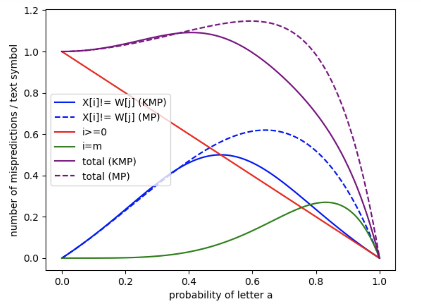
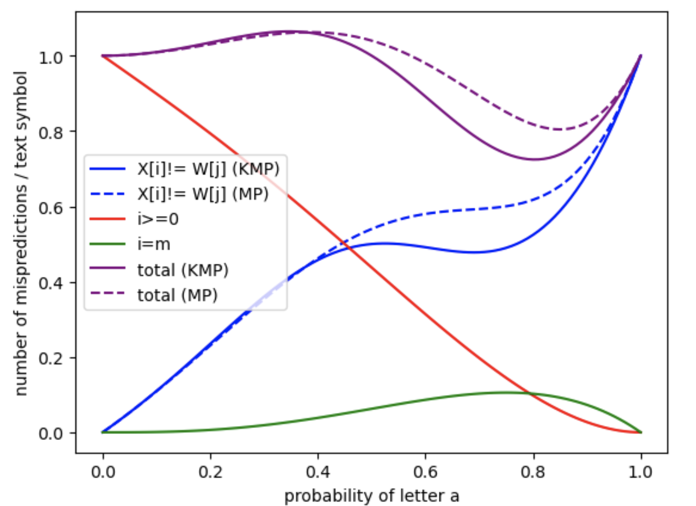
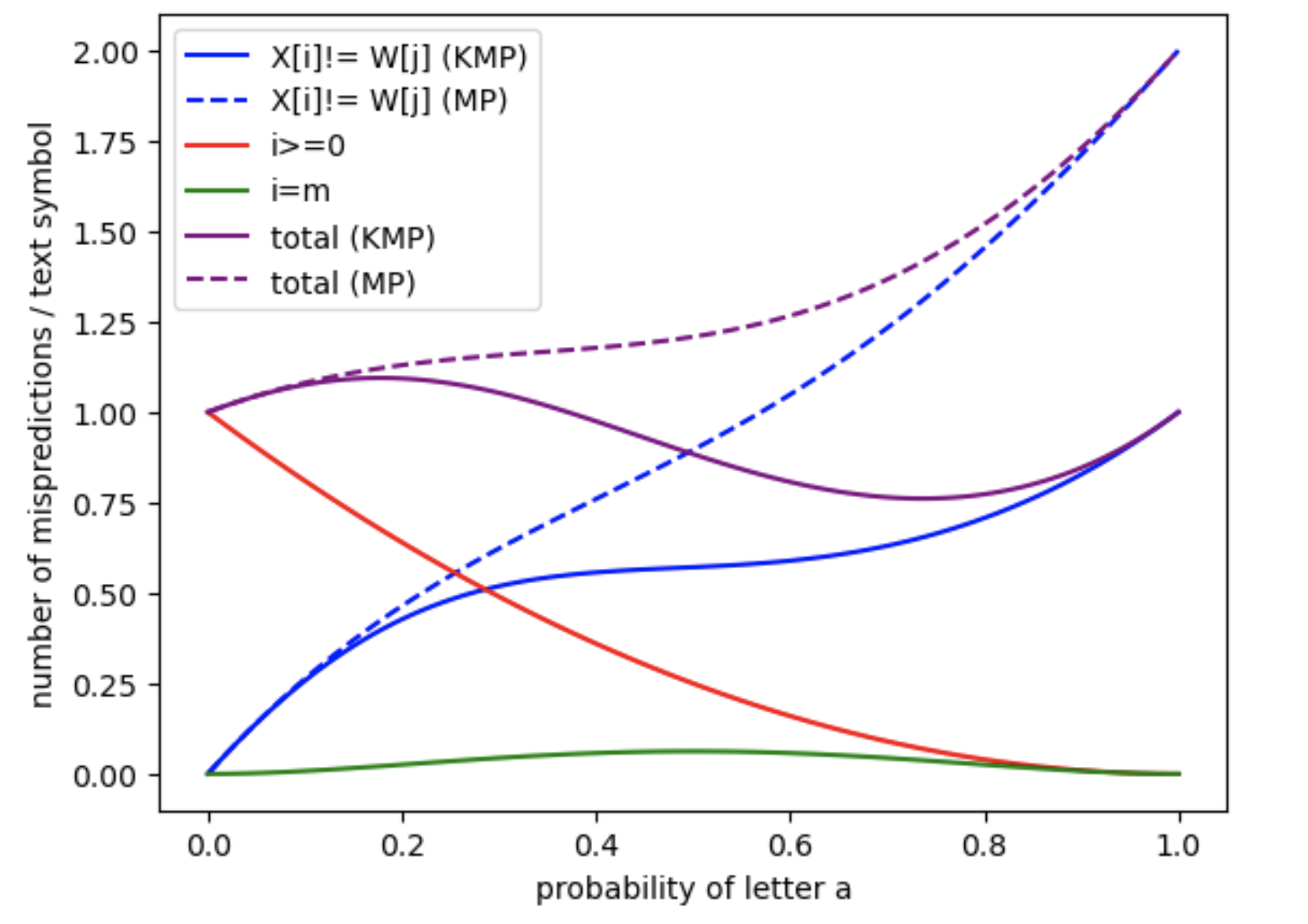
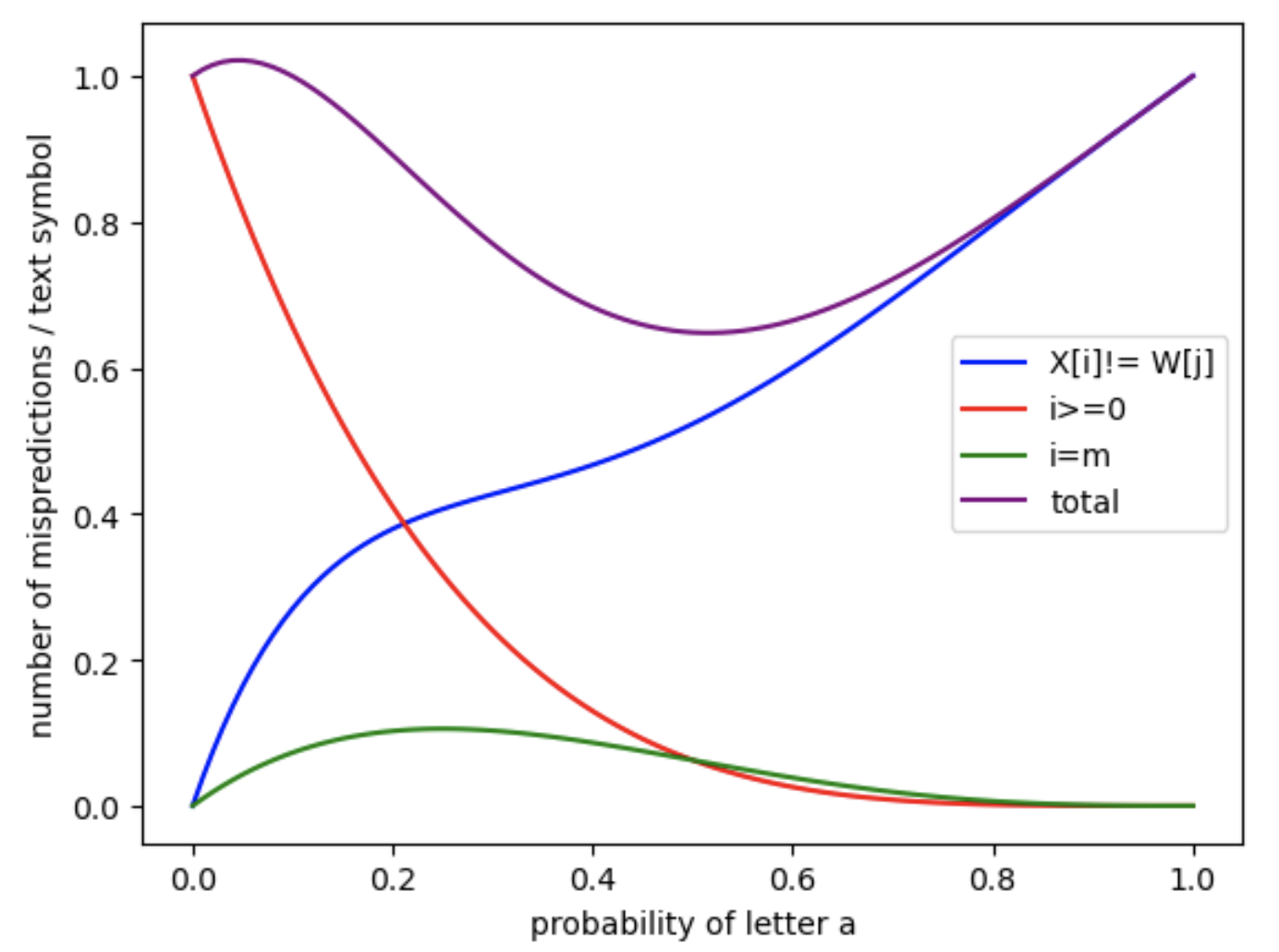
In the first series of four figures (Figure 9, Figure 10, Figure 11 and Figure 12), we apply the analytical formulas developed in the article to compute the expected number of mispredictions for each branch, as well as the total number of mispredictions across the entire matching process. These computations are performed as a function of the character probability $\pi(a)$ , which varies in the interval $[0,1]$ under the assumption of an i.i.d. binary text model over the alphabet $\{a,b\}$ . Each figure corresponds to a different pattern: $a a a a$ , $a a a b$ , $a b a b$ , and $a b b b$ . Each plot was computed in under a few seconds on a personal laptop.

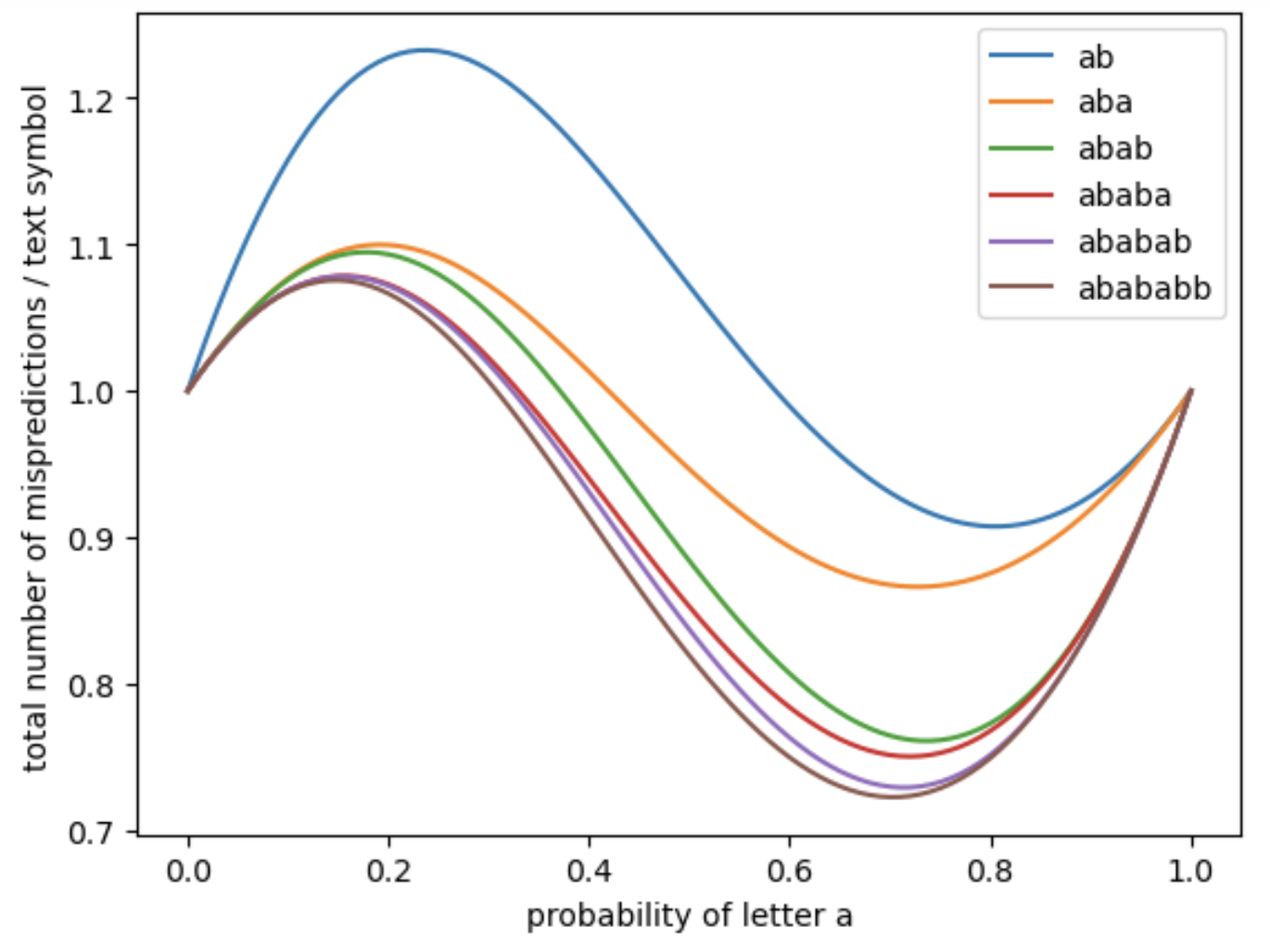
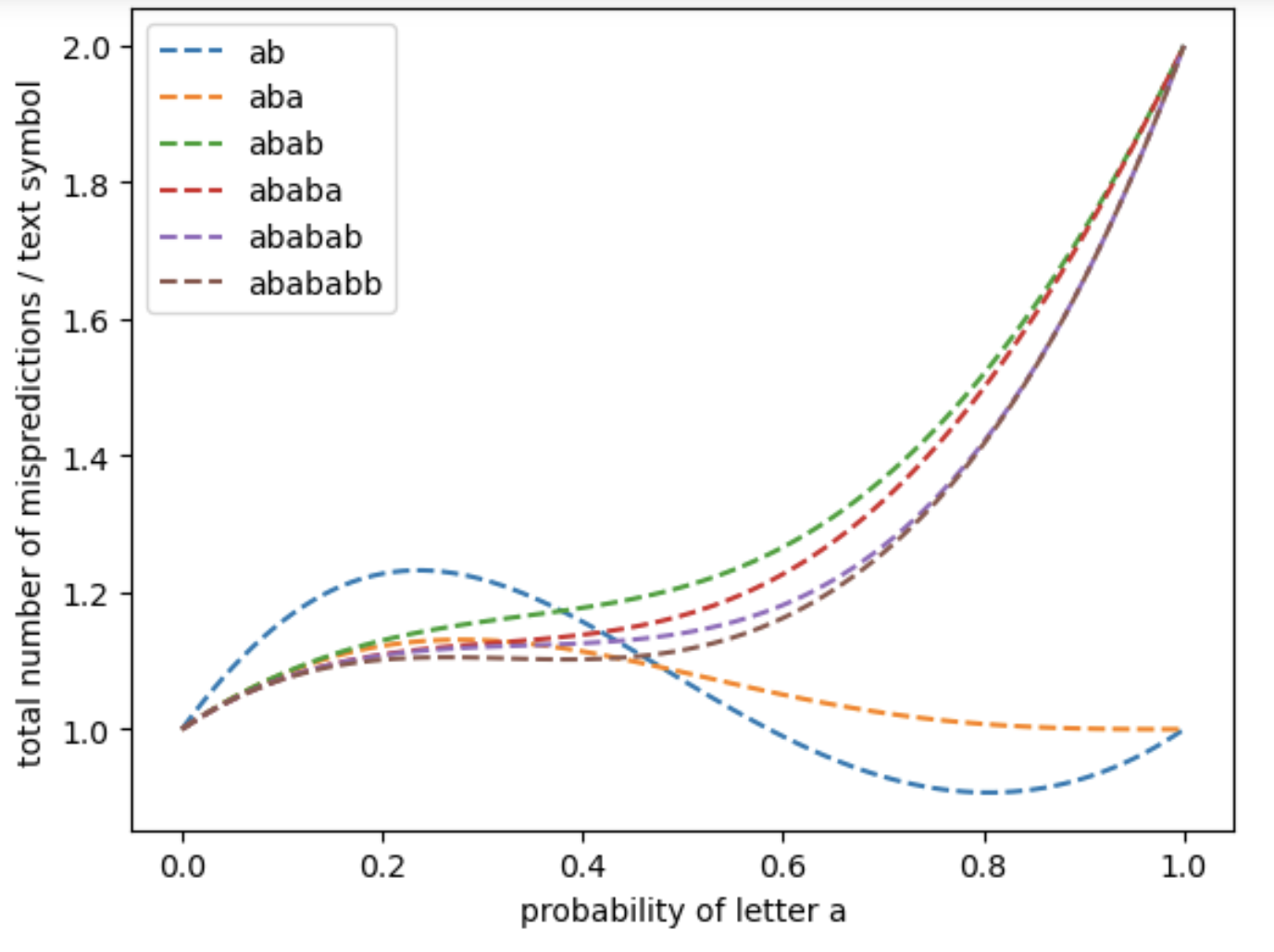
Refer to caption — Figure 9: Pattern $X=aaaa$ .

In the last two figures (Figure 13 and Figure 14), we focus on a more detailed case study. We consider all non-trivial prefixes (i.e., of length at least $2$ ) of the pattern $a b a b a b b$ , and for each prefix, we compute the expected number of mispredictions per text symbol as the text length tends to infinity. This is done for both the MP and the KMP algorithms. The results suggest a form of convergence as the length of the prefix increases. This is consistent with theoretical expectations, as longer prefixes imply that deeper states of the automaton $\mathcal{A}_{X}$ become increasingly less likely to be reached in practice.

[bib.bib1] [1] Nicolas Auger, Cyril Nicaud, and Carine Pivoteau. Good predictions are worth a few comparisons. In Nicolas Ollinger and Heribert Vollmer, editors, 33rd Symposium on Theoretical Aspects of Computer Science, STACS 2016, February 17-20, 2016, Orléans, France, volume 47 of LIPIcs, pages 12:1–12:14. Schloss Dagstuhl – Leibniz-Zentrum für Informatik, 2016. doi:10.4230/LIPICS.STACS.2016.12.

[bib.bib2] [2] Gerth Stølting Brodal and Gabriel Moruz. Tradeoffs between branch mispredictions and comparisons for sorting algorithms. In Frank K. H. A. Dehne, Alejandro López-Ortiz, and Jörg-Rüdiger Sack, editors, Algorithms and Data Structures, 9th International Workshop, WADS 2005, Waterloo, Canada, August 15-17, 2005, Proceedings, volume 3608 of Lecture Notes in Computer Science, pages 385–395. Springer, 2005. doi:10.1007/11534273_34.

[bib.bib3] [3] Maxime Crochemore, Christophe Hancart, and Thierry Lecroq. Algorithms on strings. Cambridge University Press, 2007.

[bib.bib4] [4] Maxime Crochemore and Wojciech Rytter. Text Algorithms. Oxford University Press, 1994.

[bib.bib5] [5] Dan Gusfield. Algorithms on Strings, Trees, and Sequences - Computer Science and Computational Biology. Cambridge University Press, 1997. doi:10.1017/CBO9780511574931.

[bib.bib6] [6] John L. Hennessy and David A. Patterson. Computer Architecture, Sixth Edition: A Quantitative Approach. Morgan Kaufmann Publishers Inc., 6th edition, 2017.

[bib.bib7] [7] Donald E. Knuth, James H. Morris Jr., and Vaughan R. Pratt. Fast pattern matching in strings. SIAM J. Comput., 6(2):323–350, 1977. doi:10.1137/0206024.

[bib.bib8] [8] David A. Levin, Yuval Peres, and Elizabeth L. Wilmer. Markov Chains and Mixing Times. American Mathematical Society, 2008.

[bib.bib9] [9] Conrado Martínez, Markus E. Nebel, and Sebastian Wild. Analysis of branch misses in quicksort. In Proceedings of the Twelfth Workshop on Analytic Algorithmics and Combinatorics, ANALCO 2015, San Diego, CA, USA, January 4, 2015, pages 114–128, 2015. doi:10.1137/1.9781611973761.11.

[bib.bib10] [10] Sparsh Mittal. A survey of techniques for dynamic branch prediction. Concurrency and Computation: Practice and Experience, 31, 2018.

[bib.bib11] [11] James H Morris, Jr and Vaughan R Pratt. A Linear Pattern-Matching Algorithm. Technical report, University of California, Berkeley, CA, January 1970.

[bib.bib12] [12] Mireille Régnier. Knuth-morris-pratt algorithm: An analysis. In Antoni Kreczmar and Grazyna Mirkowska, editors, Mathematical Foundations of Computer Science 1989, MFCS’89, Porabka-Kozubnik, Poland, August 28 - September 1, 1989, Proceedings, volume 379 of Lecture Notes in Computer Science, pages 431–444. Springer, 1989. doi:10.1007/3-540-51486-4_90.

[bib.bib13] [13] Mireille Régnier and Wojciech Szpankowski. Complexity of sequential pattern matching algorithms. In Michael Luby, José D. P. Rolim, and Maria J. Serna, editors, Randomization and Approximation Techniques in Computer Science, Second International Workshop, RANDOM’98, Barcelona, Spain, October 8-10, 1998, Proceedings, volume 1518 of Lecture Notes in Computer Science, pages 187–199. Springer, 1998. doi:10.1007/3-540-49543-6_16.

Branch Prediction Analysis of Morris-Pratt and Knuth-Morris-Pratt Algorithms

Abstract

Keywords and phrases:

Copyright and License:

2012 ACM Subject Classification:

DOI:

Event:

Editors:

Series and Publisher:

1 Introduction

2 Algorithms and their encoding using transducers

Algorithms MP and KMP

Associated automata

3 Expected number of letter comparisons for a given pattern

Encoding the letter comparisons with transducers

Lemma 1.

State probability and expected number of comparisons

Lemma 2.

Proposition 3.

4 Expected number of mispredictions

4.1 Mispredictions of the counter update

Proposition 4.

Proof (sketch).

Proposition 5.

4.2 Expected number of mispredictions during letter comparisons

Lemma 6.

Proposition 7.

4.3 Expected number of mispredictions of the test 𝒊≥𝟎

Proposition 8.

5 Results for small patterns, discussion and perspectives

References

6 Appendix

4.3 Expected number of mispredictions of the test $i\geq 0$