Steinhaus Filtration and Stable Paths in the Mapper

Abstract
We define a new filtration called the Steinhaus filtration built from a single cover based on a generalized Steinhaus distance, a generalization of Jaccard distance. The homology persistence module of a Steinhaus filtration with infinitely many cover elements may not be -tame, even when the covers are in a totally bounded space. While this may pose a challenge to derive stability results, we show that the Steinhaus filtration is stable when the cover is finite. We show that while the Čech and Steinhaus filtrations are not isomorphic in general, they are isomorphic for a finite point set in dimension one. Furthermore, the VR filtration completely determines the -skeleton of the Steinhaus filtration in arbitrary dimension.
We then develop a language and theory for stable paths within the Steinhaus filtration. We demonstrate how the framework can be applied to several applications where a standard metric may not be defined but a cover is readily available. We introduce a new perspective for modeling recommendation system datasets. As an example, we look at a movies dataset and we find the stable paths identified in our framework represent a sequence of movies constituting a gentle transition and ordering from one genre to another.
For explainable machine learning, we apply the Mapper algorithm for model induction by building a filtration from a single Mapper complex, and provide explanations in the form of stable paths between subpopulations. For illustration, we build a Mapper complex from a supervised machine learning model trained on the FashionMNIST dataset. Stable paths in the Steinhaus filtration provide improved explanations of relationships between subpopulations of images.
Keywords and phrases:
Cover and nerve, Jaccard distance, persistence stability, Mapper, recommender systems, explainable machine learningCopyright and License:
Amber Thrall; licensed under Creative Commons License CC-BY 4.0
2012 ACM Subject Classification:
Theory of computationSupplementary Material:
Software: https://github.com/AmberThrall/SteinhausNotebooks/archived at
Acknowledgements:
Broussard, Krishnamoorthy, and Saul acknowledge funding from the US National Science Foundation through grants 1661348 and 1819229. Part of the research described in this paper was conducted under the Laboratory Directed Research and Development Program at Pacific Northwest National Laboratory, a multiprogram national laboratory operated by Battelle for the U.S. Department of Energy.Editors:
Oswin Aichholzer and Haitao WangSeries and Publisher:
1 Introduction
The need to rigorously seed a solution with a notion of stability in topological data analysis (TDA) has been addressed primarily using topological persistence [4, 11, 17]. Persistence arises when we work with a sequence of objects built on a dataset, a filtration, rather than with a single object. One line of focus of this work has been on estimating the homology of the dataset. This typically manifests itself as examining the persistent homology represented as a diagram or barcode, with interpretations of zeroth and first homology as capturing significant clusters and holes, respectively [1, 14, 15, 37]. In practice it is not always clear how to interpret higher dimensional homology (even holes might not make obvious sense in certain cases). A growing focus is to use persistence diagrams to help compare different datasets rather than interpret individual homology groups [2, 8, 34].
The implicit assumption in most such TDA applications is that the data is endowed with a natural metric, e.g., points exist in a high-dimensional space or pairwise distances are available. In certain applications, it is also not clear how one could assign a meaningful metric. For example, memberships of people in groups of interest is captured simply as sets specifying who belongs in each group. An instance of such data is that of recommendation systems, e.g., as used in Netflix to recommend movies to the customer. Graph based recommendation systems have been an area of recent research. Usually these systems are modeled as a bipartite graph with one set of nodes representing recommendees and the other representing recommendations. In practice, these systems are augmented in bespoke ways to accommodate whichever type of data is available. It is highly desirable to analyze the structure without prescribing some ill-fit or incomplete metric to the data.
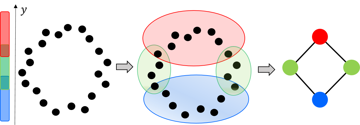
Another TDA approach for structure discovery and visualization of high-dimensional data is based on a construction called Mapper [32]. Defined as the nerve of a refined pullback cover of the data (See Figure 1), Mapper has found increasing use in diverse applications in the past several years [23]. Attention has recently focused on interpreting parts of the -skeleton of the Mapper complex, which is a simplicial complex, as significant features of the data. Paths, flares, and cycles have been investigated in this context [21, 26, 33]. The framework of persistence has been applied to this construction to define a multi-scale Mapper, which permits one to derive results on stability of such features [13]. At the same time, the associated computational framework remains unwieldy and still most applications base their interpretations on a single Mapper object.
The Mapper construction works with covers. By default, one starts with overlapping hypercubes that cover a parameter space (usually a subset of for some dimension ) and consider the pullback of this cover to the space of data. In recommendation systems, the cover is just a collection of abstract sets providing membership info. Could we define a topological construction on such abstract covers that still reveals the topology of the dataset?
We could study paths in this construction, but as the topological constructions are noisy, we would want to define a notion of stability for such paths. With this goal in mind, could we define a filtration from the abstract cover? But unlike in the setting of, e.g., multiscale Mapper [13], we do not have a sequence of covers (called a tower of covers) – we want to work with a single cover. How do we define a filtration on a single abstract cover? And could we prove is is stable? Finally, could we use our construction on real data?
1.1 Our Contributions
We introduce a new type of filtration defined on a single abstract cover. Termed Steinhaus filtration, our construction uses Steinhaus distances between elements of the cover. We generalize the Steinhaus distance between two elements to those of multiple elements in the cover, and define a filtration on a single cover using the generalized Steinhaus distance as the filtration index. The homology persistence module of a Steinhaus filtration with infinitely many cover elements may not be -tame, even when the covers are in a totally bounded space (Lemma 3.1). While this may pose a challenge to derive stability results, we show a stability result on the Steinhaus filtration when the cover is finite – the largest change in generalized Steinhaus distance provides an upper bound for the bottleneck distance of their homologies (Theorem 3.10). We prove that in 1-dimension the Steinhaus filtration is isomorphic to the standard Čech filtration built on the dataset (Theorem 4.1) and independently that the Vietoris-Rips (VR) filtration completely determines the -skeleton of the Steinhaus filtration in arbitrary dimensions (Lemma 4.2). We show by example that the Steinhaus filtration is not isomorphic to the Čech filtration in higher dimensions (Proposition 4.3).
This filtration is quite general, and enables the computation of persistent homology for datasets without requiring strong assumptions or defining ill-fit metrics. With real life applications in mind, we study paths in our construction. Paths provide intuitive explanations of the relationships between the objects that the terminal vertices represent. Our perspective of path analysis is that shortest may not be more descriptive – see Figure 2 for an illustration. Instead, we define a notion of stability of paths in the Steinhaus filtration. Under this notion, a stable path is analogous to a highly persistent feature as identified by persistent homology.
We demonstrate the utility of stable paths in Steinhaus filtrations on two real life applications: a problem in movie recommendation system and Mapper. We first show how recommendation systems can be modeled using the Steinhaus filtration, and then show how stable paths within this filtration suggest a sequence of movies that represent a “smooth” transition from one genre to another (Section 6.1). We then define an extension of the traditional Mapper [32] termed the Steinhaus Mapper Filtration, and show how its stable paths provide valuable explanations of populations in the Mapper complex, focusing on explainable machine learning (Section 6.2). Code for our computations is available at https://github.com/AmberThrall/SteinhausNotebooks/.
1.2 Related Work
Cavanna and Sheehy [7] developed theory for a cover filtration, built from a cover of a filtered simplicial complex. But we work from more general covers of arbitrary spaces.
We are inspired by similar goals as those of previous work addressing stability of the Mapper construction by Dey, Mémoli, and Wang [13] and by Carrière and Oudot [6]. Our goal is to provide some consistency, and thus interpretability, to the Mapper construction. We incorporate ideas of persistence in a different manner into our construction using a single cover, which considerably reduces the effort of generating results.
The multi-scale Mapper defined by Dey, Mémoli, and Wang [13] builds a filtration on the Mapper complex by varying the parameters of a cover. This construction yields nice stability properties, but is unwieldy in practice and difficult to interpret. Carrière, Michel, and Oudot develop ways based on extended persistence to automatically select a hypercube cover that best captures the topology of the data [5]. This approach constructs one final Mapper that is easy to interpret, but is restricted to the use of hypercube covers, which is just one option of myriad potential covering schemes.
Kalyanaraman, Kamruzzaman, and Krishnamoorthy developed methods for tracking populations within the Mapper graph by identifying interesting paths [19] and interesting flares [20]. Interesting paths maximize an interestingness score, and are manifested in the Mapper graph as long paths that track particular populations that show trending behavior. Flares capture subpopulations that diverge, i.e., show branching behavior. In our context, we are interested in shorter paths, under the assumption that they provide the most succinct explanations for relationships between subpopulations.
Our work is similar to that of Parthasarathy, Sivakoff, Tian, and Wang [27] in that they use the Jaccard Index of an observed graph to estimate the geodesic distance of the underlying graph. We take an approach more akin to persistence and make far fewer assumptions.We cannot make rigorous estimates of distances but provide many possible representative paths.
The notion of S-paths [29] is similar to stable paths if we model covers as hypergraphs, and vice versa. Stable paths incorporate the size of each cover element (or hyperedges), normalizing the weights by relative size. This perspective allows us to compare different parts of the resulting structure which may have wildly difference sizes of covers. In this context, a large overlap of small elements is considered more meaningful than a proportionally small intersection of large elements.
In Section 6.1, we show how the Steinhaus filtration and stable paths can be applied in the context of recommendation systems. Our viewpoint on recommendation systems is similar to work of graph-based recommendation systems. This is an active area of research and we believe our new perspective of interpreting such systems as covers and filtrations will yield useful tools for advancing the field. The general approach of graph-based recommendation systems is to model the data as a bipartite graph, with one set of nodes representing the recommendation items and the other set representing the recommendees. We can interpret a bipartite graph as a cover, either with elements being the recommendees covering the items, or elements being the items covering the recommendees.
2 Steinhaus Filtrations
We define the Steinhaus distance, a generalization of the Jaccard distance between two sets, and further generalize it to an arbitrary collection of subsets of a cover. These generalizations take a measure and assume that all sets are taken mod differences by sets of measure .
Definition 2.1 (Steinhaus Distance [24]).
The Steinhaus distance between sets given a measure is .
This distance lies in , is when sets are equal and when they do not intersect.
Definition 2.2 (Generalized Steinhaus distance).
Define the generalized Steinhaus distance of a collection of sets as .
We make use of this generalized distance to associate birth times to simplices in a nerve. Given a cover, we define the Steinhaus filtration as the filtration induced from sublevel sets of the generalized Steinhaus distance function. In other words, consider a cover of the space and the nerve of this cover. For each simplex in the nerve, we assign as birth time the value of its Steinhaus distance of its corresponding cover elements. This filtration captures information about similarity of cover elements and overall structure of the cover.
Definition 2.3 (Nerve).
A nerve of a cover is an abstract simplicial complex defined such that each subset with , defines a simplex if . In this construction, each cover element defines a vertex.
Definition 2.4 (Steinhaus Nerve).
The Steinhaus nerve of a cover , denoted , is defined as the nerve of with each simplex assigned their generalized Steinhaus distance as weight:
Note that by definition for every simplex . We will use when the cover is evident from context. The weighting scheme satisfies the conditions of a filtration.
Theorem 2.5.
The Steinhaus nerve of a cover is a filtered simplicial complex.
Proof.
This proof makes use of standard set theory results. Let be an arbitrary cover of some set and let be its Steinhaus nerve. We consider as a filtration by assigning as the birth time of simplex its weight . To show this is indeed a filtration, we focus on a single simplex and a face to show that the face always appears in the filtration before the simplex.
Suppose is generated from cover elements over some index set . Let a face be generated by cover elements indexed by a subset . The birth time of is
Clearly, with , we have that and . It follows then that . With denoting the subcomplex that includes all simplices in with birth time at most , for any with , we have . Hence is a monotonic filtration. Following this result, we refer to the construction as the Steinhaus filtration.
We could study an adaptation of Steinhaus filtration to an analog of the VR complex by building a weighted clique rank filtration from the -skeleton of the Steinhaus filtration [28]. This adaptation drastically reduces the number of intersection and union checks required for the construction. The weight rank clique filtration is a way of generating a flag filtration from a weighted graph [28]. We can use this idea to build a VR analog of the Steinhaus filtration.
3 Stability
We provide a brief overview of persistence modules and the bottleneck distance. For details, see the book by Chazal, de Silva, Glisse, and Oudot [9].
Given a poset , we define a persistence module over to be an indexed family of vector spaces with a family of linear maps that satisfy whenever . The homologies of the Steinhaus filtered simplicial complex defines a persistence module where each space is the homology of the simplicial complex consisting of simplices whose corresponding Steinhaus distance is at most . Herein, we use simplicial homology with coefficients in some field .
Given two persistence modules and over and , a homomorphism of degree is a collection of linear maps such that . We denote the set of homomorphisms of degree by . The composition of a homomorphism of degree and a homomorphism of degree is a homomorphism of degree given by the composition of their linear maps. For , a crucial endomorphism of degree is the shift map given by the maps
We say that two persistence modules and are -interleaved if there are homomorphisms and such that and .
When a persistence module is -tame, i.e., whenever , then the persistence module decomposes into the direct sum of interval modules Each term represent the birth time and death time of a particular feature. This decomposition is often represented by the multiset of points in the extended plane . This multiset is called the persistence diagram of and denoted .
In typical applications, the simplicial complex is finite. As a result, their homologies are finite and any map between their homologies will have finite rank. In other words, in typical cases the homologies of the Steinhaus filtration will be -tame. However, if we allow for infinitely many cover elements then may not be -tame.
Lemma 3.1.
There is a Steinhaus filtered simplicial complex in a totally bounded space whose homology persistence module is not -tame.
Proof.
Consider the Mapper complex in Figure 3. Each cover element is a rectangle of size
with rectangular intersections of size and . Under the Lebesgue measure, we get the Steinhaus distances of and . Hence, under our Steinhaus filtration the cycles going around the red-green-red-green diamonds in the complex are born at 200/210 and the remaining cycles are born at 366/381. Since these cycles form a linearly independent set, we get that in the first homology persistence module the map from to has infinite rank.
We modify this construction to get a non -tame example in a totally bounded space by shrinking each subsequent cover by factor of two. Thus, if we make the covers have sizes
and position them such that
then the covers are contained in a finite rectangle and the map in the first homology persistence module from to will have infinite rank.
Definition 3.2.
A partial matching between multisets and is a collection of pairs such that for every , there is at most one such that and for every , there is at most one such that .
Let be the diagonal. The cost of a partial matching is given by
Definition 3.3 (Bottleneck distance).
The bottleneck distance between and is given by
Theorem 3.4 ([9]).
If is a -tame persistence module then it has a well-defined persistence diagram . If are -tame persistence modules that are -interleaved then .
We define a multivalued map between and , denoted , to be a subset of such that the projection onto is surjective. A multivalued map is said to be a correspondence if the projection onto is surjective, or equivalently,
Definition 3.5 (-simplicial [10]).
Let and be filtered simplicial complexes with vertex sets and . A multivalued map is -simplicial if for any and any simplex , every finite subset of is a simplex of .
Proposition 3.6 ([10]).
Let and be filtered simplicial complexes with vertex sets and . If is a correspondence such that and are both -simplicial, then they induce an -interleaving between and given by and .
Let and be two Steinhaus filtered simplicial complexes. Given a correspondence , we define the distortion of to be
i.e., the largest change in birth times across each simplex. We then define the pseudometric by finding the correspondence with the smallest distortion:
Lemma 3.7.
is a pseudometric.
does not satisfy the positivity requirement to be a metric. Consider the covers and given in Figure 4. The simplicial complexes are not isomorphic, but .
Proposition 3.9.
Let and be two Steinhaus filtered simplicial complexes. If , then the persistence modules and are -interleaved.
Theorem 3.10.
Let and be two Steinhaus filtered simplicial complexes with -tame homology persistence modules. Then
4 Equivalence
To situate the Steinhaus filtration in the context of standard filtrations built on point clouds in Euclidean space, we wish to show the equivalence of the Steinhaus filtration to the Čech and VR filtrations under certain conditions. We first show that the Čech filtration on a finite set of points in dimension one, i.e., the nerve of balls with radius around each point and over a sequence of , and the Steinhaus Nerve constructed from the terminal cover of the Čech filtration are isomorphic (see Theorem 4.1).
We provide experimental evidence for the -skeletons of the Steinhaus filtration and the VR filtration being isomorphic. We prove one direction of this equivalence in arbitrary dimension – that the VR filtration completely determines the -skeleton of the Steinhaus filtration (see Lemma 4.2). We prove by example that the Steinhaus filtration and the Čech filtration in two (or higher) dimension(s) may not be isomorphic (see Proposition 4.3).
Let be cover of by balls of radius centered on points in . The Čech complex is the nerve of this cover. The Čech filtration is sequence of simplicial complexes for all .
Theorem 4.1.
Given a finite dataset in dimension one and some radius the Čech filtration constructed from is isomorphic to the Steinhaus filtration on constructed from , given the Lebesgue (i.e., volume) measure.
Proof.
We set as birth radius of the simplex defined by , computed as
since in 1D space the simplex is born when balls around the two outermost points intersect.
Let be the set of balls of radius centered on the set . Recall that we are using the Steinhaus distance for Lebesgue measure, so computes volume here. Then the generalized Steinhaus distance for those balls is given by , since the mutual intersection of all the balls in this one dimensional space is the interval bounded by the minimum right endpoint of all the balls and the maximum of all left endpoints of all the balls and the union of all the balls has the minimum left endpoint amongst left endpoints and maximum right endpoint amongst right endpoints.
Solving for , we get giving a bijection between birth times.
Now since and , . Also, decreases monotonically over the range . Thus, increases monotonically on . Thus, if we order the subsets of by increasing birth radius , then the Steinhaus distances are also in increasing order, showing the isomorphism.
Lemma 4.2.
There is a map from the birth time of an edge in the VR filtration to its birth time in the Steinhaus filtration. Hence the VR filtration determines the -skeleton of the Steinhaus filtration in arbitrary dimensions.
Proof.
The volume of the intersection of two hyperspheres was derived by Li [22]. The volume of intersection of two hyperspheres of equal radius in with centers distance apart is defined as
where is the gamma function and is the regularized incomplete beta function:
We can reduce this equation to
We then compute the Steinhaus distance with Lebesgue measure of two spheres in and radius with Euclidean distance apart as
This equation provides a mapping from the birth time of the edge in the VR filtration to the birth time of the edge in the Steinhaus filtration. Once an and are chosen, the equation readily reduces, producing the birth times of a simplex in the Steinhaus filtration.
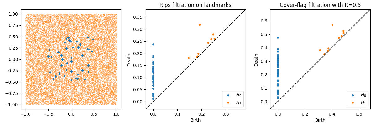
Next we provide detailed experimental results suggesting that the -skeletons of the Steinhaus and the VR filtrations are isomorphic. We estimate the area of intersection of 1-spheres using Monte Carlo integration with uniform sampling. The first plot in Figure 5 shows the 50 landmark points along with 20,000 points uniformly sampled around the landmarks for ease of computation. The middle plot shows the persistence diagrams of dimension 0 and 1 for the VR filtration on the landmarks. Finally, we show the Steinhaus filtration on the landmarks using balls with radii 0.5 as the covers.
Proposition 4.3.
The Čech and Steinhaus filtrations are not isomorphic in general.
Proof.
Let be the four corners of a unit square. We construct a cover where at each point in there is a ball of radius one (see Figure 6). In the Steinhaus filtration, four 2-simplices are born approximately at 0.935 before the 3-simplex is born around 0.959 under the volume measure. However, in the Čech complex the 2-simplices are born at the same time as the 3-simplex.
5 Stable Paths
We develop a theory of stable paths within a Steinhaus filtration. We provide an algorithm for computing a most stable path from one vertex to another. Note that a most stable path might not be a shortest path in terms of number of edges. Conversely, a shortest path might not be highly stable. Since the two objectives are at odds with each other, we provide an algorithm to identify a family of shortest paths as we vary the stability level.
We were studying shortest paths in a Mapper graph constructed on a machine learning model as ways to illustrate the relations between the data as identified by the model. In this context, shortest paths found could have low Steinhaus distance, and thus could be considered noise. This motivated our desire to find stable paths, as they would intuitively be most representative of data and stable with respect to changing or data.
Definition 5.1 (-Stable Path).
A path is said to be -stable for Steinhaus distance if where is the Steinhaus distance associated with edge .
It follows that a -stable path is also -stable for any . Also, a -stable path is more stable than a -stable path when . In this case, we have a higher confidence that the edges in do exist, and are not due to noise, than the edges in .
Definition 5.2 (Most Stable Path).
Given a pair of vertices and , a most stable - path is a -stable path between and for the smallest value of . If there are multiple - paths at the same minimum value, a shortest path among them is defined as a most stable path.
The problem of finding the most stable - path can be solved as a minimax path problem on an undirected graph, which can solved efficiently using, e.g., range minimum queries [12].
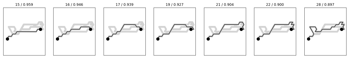
We are then left with two paths between vertices and , the shortest and the most stable. As these two notions, stable and short, are at odds with each other, we are interested in computing the entire Pareto frontier between the short and stable path. Algorithm 1 identifies the Pareto frontier, and its sample output is shown in Figure 7.
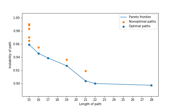
The blue points in Figure 7 are on the Pareto frontier, while the orange points are the pairs that get replaced from the LIST in the course of the algorithm. We then visualize the paths on the Pareto frontier in Figure 8. Continuing our analogy to persistence, the path corresponding to a point on the Pareto frontier which sees a steep rise to the left is considered highly persistent, e.g., the path with length on the frontier.
6 Applications
We apply the Steinhaus filtration and stable paths to recommendation systems and Mapper analysis. We show how recommendation systems can be modeled using the Steinhaus filtration and then show how stable paths in this filtration can answer the question what movies should I show my friend first, to wean them into my favorite (but potentially weird) movie? We then define an extension of the traditional Mapper complex [32, 6] called the Steinhaus Mapper Filtration, and show how stable paths within this filtration can provide valuable explanations of populations in the Mapper construction. As a direct illustration, we focus on the case of explainable machine learning, where the Mapper complex is constructed with a supervised machine learning model as the filter function, and address the question what can we learn about the model?
6.1 Recommendation Systems
We apply the Steinhaus filtration to a recommendation system dataset and employ the stable paths analysis to compute sequences of movies that ease viewers from one title to another title. Suppose you have only ever seen the movie Mulan and your partner wants to show you Moulin Rouge. It would be jarring to watch that movie, so your partner might gently build up to it by showing movies similar to both Mulan and Moulin Rouge. We compute stable paths that identify such a gentle sequence.
We use the MovieLens-20m dataset [18], comprised of 20 million ratings by 138,493 users of 27,278 movies. Often, these types of datasets are interpreted as bipartite graphs. We note that a bipartite graph can be equivalently represented as a covering of one node set with the other, and apply the Steinhaus filtration to build a filtration. In our case, we interpret each movie as a cover element of the users who have rated the movie. To reduce computational expenses and noise, we remove all movies with less than 10 ratings and then sample 4000 movies at random from the remaining movies.
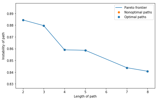
Figure 9 shows the computed Pareto frontier of stable paths for the case of Mulan and Moulin Rouge. In Table 1, we show two stable paths. The stable path with length 4 is found after a large drop in instability. As the length and stability must be traded off, we think this would be a decent path to choose if you want to optimize both. The second path is the most stable. For readers familiar with the movies, the relationship between each edge is clear.
| Shortest Path | Most Stable Path |
| 1. Mulan (1998) 2. Dumbo (1941) 3. The Sound of Music (1965) 4. Moulin Rouge (2001) | 1. Mulan (1998) 2. Robin Hood (1973) 3. Dumbo (1941) 4. The Sound of Music (1965) 5. Gone with the Wind (1939) 6. Psycho (1960) 7. High Fidelity (2000) 8. Moulin Rouge (2001) |
6.2 Steinhaus Mapper Filtration
We develop a method of model induction for inspecting a machine learning model. The goal is to develop an understanding of the model structure by characterizing the relationship between the feature space and the prediction space. The Mapper construction [32] is aptly suited for visualizing this functional structure.
This application is based on the work of using paths in the Mapper graph to provide explanations for supervised machine learning models [31]. In a similar approach, Rathore, Chalapathi, Palande, and Wang [30] used the Mapper construction to visually explore shapes of activations in deep learning. They focused mostly on bifurcations in the Mapper graph, and did not directly address the question of stability of the features. We build a Mapper from the predicted probability space of a logistic regression model. We then extend that Mapper to be a Steinhaus Mapper Filtration and analyze its stable paths.
Given topological spaces , function , and a cover of , the Mapper complex is the nerve of the refined, i.e., with each cover element split into path-connected components, pullback cover of . Typically, a clustering algorithm is used to compute the pullback of each cover element.
Definition 6.1 (Steinhaus Mapper filtration).
Given data , a function , and a cover of , we define the Steinhaus Mapper as the Steinhaus nerve (Definition 2.4) of the refined pullback cover of :
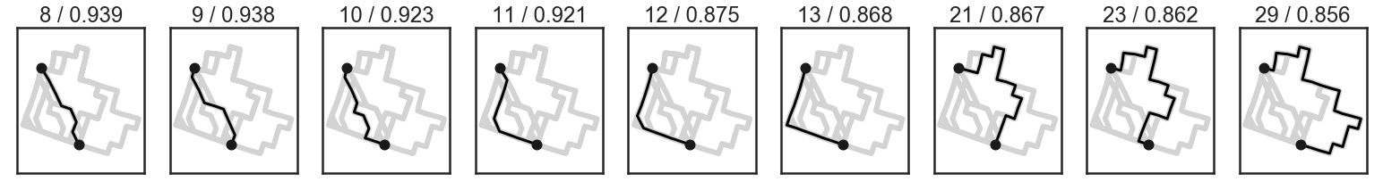
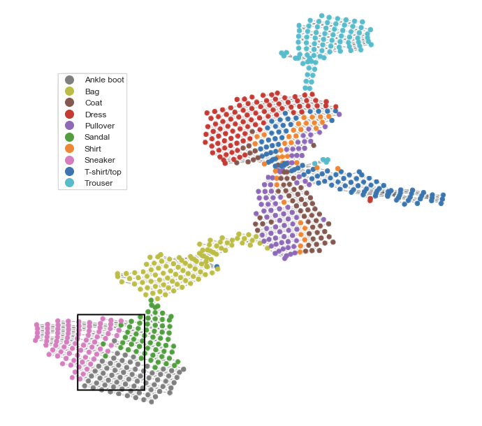
Figure 10 shows the Steinhaus Mapper filtration constructed from a logistic regression model built on the Fashion-MNIST dataset [36], with 70,000 images of clothing items from 10 classes. Each image is pixels. The Fashion-MNIST dataset is typically considered to be a more difficult application than the MNIST handwritten digits.
We first reduce the dataset to 100 dimensions using Principal Components Analysis, and then a logistic regression classifier with regularization is trained on the reduced data using 5-fold cross validation on a training set of 60,000 images. The model evaluated at 93% accuracy on the remaining 10,000 images. We then extract the 10-dimensional predicted probability space and use UMAP [25] to reduce it to 2 dimensions. This 2-dimensional space is taken as the filter function of the Mapper complex, using a cover consisting of 40 bins along each dimension with 50% overlap between each bin. DBSCAN is used as the clustering algorithm in the refinement step [16]. KeplerMapper [35] is used to construct the Mapper complex. Finally, the cover is extracted and the Steinhaus Mapper filtration is constructed.
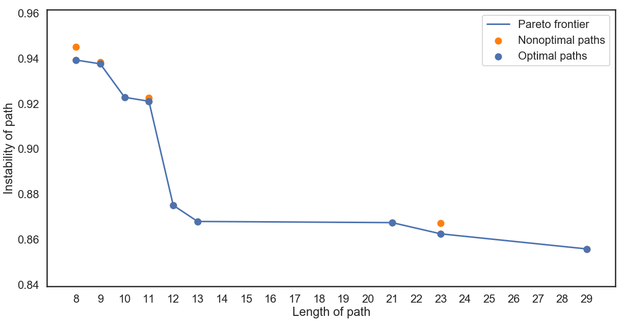
To illustrate path explanations, we take two vertices selected from the sneaker and ankle boot regions of the resulting graph. The three regions of shoes (sneaker, ankle boot, and sandals) are understandably confusing to the model, and we are interested in where these confusions arise. Figure 11 shows the paths associated with the Pareto frontier (Figure 12).
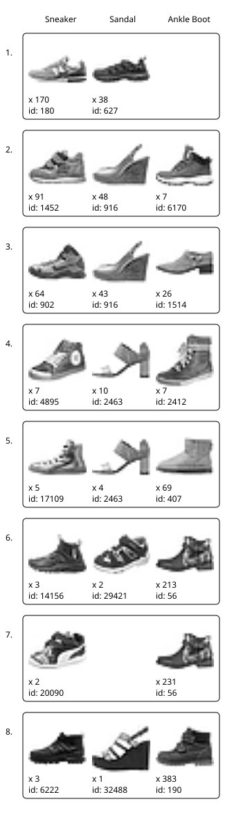
Figure 13 shows representatives from each vertex in the path for the shortest and the stable path with length 12. Each row corresponds to one vertex and the columns show a representative from each class represented in the vertex. Each image shows the multiplicity of that type of shoe in the vertex.
 |
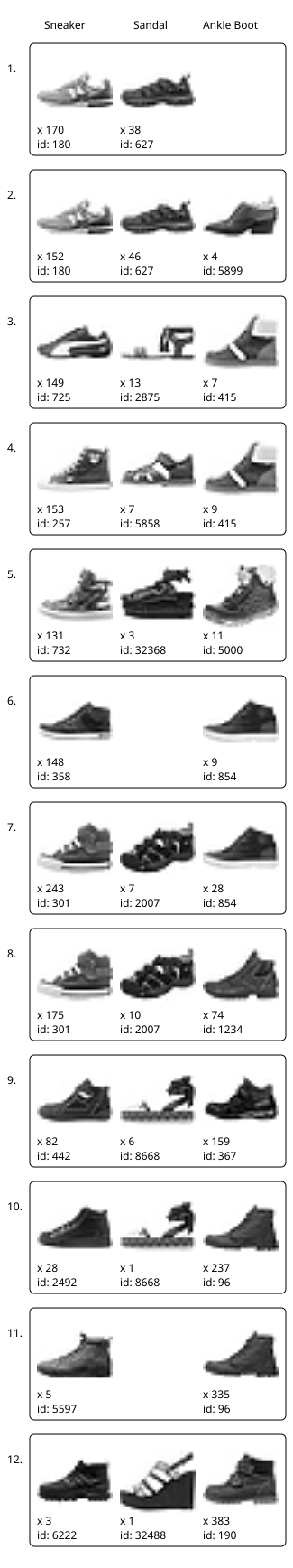 |
In both paths, vertices start with mostly sneakers and sneaker-like sandals. They then transition to contain larger proportions of ankle boots, with all three classes showing higher cut tops or high heels.
Along each path we see the relationships between nodes change. In the most stable path (Right), we see slow transition from sneaker to ankle boot space, with some sandals spread throughout. Along the path, shoes from all three classes become taller. Near the middle, images from sneakers and ankle boots are indistinguishable.
7 Discussion
We introduced the Steinhaus filtration, a new kind of filtration that enables application of TDA to previously inaccessible types of data. We then developed a theory of stable paths in the Steinhaus filtration, and provide algorithms for computing the Pareto frontier between short and stable paths. As proof of their utility to real world applications, we show how these two ideas can be applied to the analysis of recommendation systems and of Mapper in the context of explainable machine learning.
Our results suggest many new questions. The application of recommendation systems leaves us curious if the Steinhaus filtration along with new results such as the one on predicting links in graphs using persistent homology [3] could help answer the main question in recommendation system research: what item to recommend to the user next?
While paths and connected components are most amenable to practical interpretations, could other structures in the Steinhaus filtration also suggest insights? What would holes and loops in the Steinhaus filtration for recommendation systems mean?
We showed that when the cover is finite, the Steinhaus filtration is stable to small changes within the cover. The example showing non -tameness for instances with infinite covers even when it is in a totally bounded space motivates this following question: can we find a finite subcover that approximates such infinite covers?
References
- [1] Henry Adams and Gunnar Carlsson. On the nonlinear statistics of range image patches. SIAM Journal on Imaging Sciences, 2(1):110–117, 2009. doi:10.1137/070711669.
- [2] Henry Adams, Tegan Emerson, Michael Kirby, Rachel Neville, Chris Peterson, Patrick Shipman, Sofya Chepushtanova, Eric Hanson, Francis Motta, and Lori Ziegelmeier. Persistence Images: A stable vector representation of persistent homology. Journal of Machine Learning Research, 18(8):1–35, 2017. URL: http://jmlr.org/papers/v18/16-337.html.
- [3] Sumit Bhatia, Bapi Chatterjee, Deepak Nathani, and Manohar Kaul. A persistent homology perspective to the link prediction problem. In Hocine Cherifi, Sabrina Gaito, José Fernendo Mendes, Esteban Moro, and Luis Mateus Rocha, editors, Complex Networks and Their Applications VIII, pages 27–39, Cham, 2020. Springer International Publishing. arXiv:1811.04049.
- [4] Gunnar Carlsson. Topology and data. Bulletin of the American Mathematical Society, 46(2):255–308, January 2009. doi:10.1090/s0273-0979-09-01249-x.
- [5] Mathieu Carrière, Bertrand Michel, and Steve Oudot. Statistical analysis and parameter selection for Mapper. Journal of Machine Learning Research, 19(12):1–39, 2018. arXiv:1706.00204.
- [6] Mathieu Carrière and Steve Oudot. Structure and stability of the one-dimensional Mapper. Foundations of Computational Mathematics, 18:1333–1396, October 2018. doi:10.1007/s10208-017-9370-z.
- [7] Nicholas J Cavanna and Donald R Sheehy. Persistent nerves revisited. Young Researchers Forum at Symposium of Computational Geometry, 2017. URL: http://donsheehy.net/research/cavanna17peristent_yrf.pdf.
- [8] Frédéric Chazal, David Cohen-Steiner, Leonidas J. Guibas, Facundo Mémoli, and Steve Y. Oudot. Gromov-Hausdorff stable signatures for shapes using persistence. In Proceedings of the Symposium on Geometry Processing, SGP ’09, pages 1393–1403, Aire-la-Ville, Switzerland, Switzerland, 2009. Eurographics Association. doi:10.1111/j.1467-8659.2009.01516.x.
- [9] Frédéric Chazal, Vin de Silva, Marc Glisse, and Steve Oudot. The Structure and Stability of Persistence Modules. SpringerBriefs in Mathematics. Springer Cham, 1 edition, 2016. doi:10.1007/978-3-319-42545-0.
- [10] Frédéric Chazal, Vin de Silva, and Steve Oudot. Persistence stability for geometric complexes. Geometriae Dedicata, 173:193–214, 2014. doi:10.1007/s10711-013-9937-z.
- [11] Frédéric Chazal and Bertrand Michel. An introduction to Topological Data Analysis: Fundamental and practical aspects for data scientists. Frontiers in Artificial Intelligence, 4, 2021. doi:10.3389/frai.2021.667963.
- [12] Erik D. Demaine, Gad M. Landau, and Oren Weimann. On Cartesian trees and range minimum queries. In Susanne Albers, Alberto Marchetti-Spaccamela, Yossi Matias, Sotiris Nikoletseas, and Wolfgang Thomas, editors, Automata, Languages and Programming, pages 341–353, Berlin, Heidelberg, 2009. Springer Berlin Heidelberg. doi:10.1007/978-3-642-02927-1_29.
- [13] Tamal K. Dey, Facundo Mémoli, and Yusu Wang. Multiscale Mapper: Topological summarization via codomain covers. In Proceedings of the Twenty-Seventh Annual ACM-SIAM Symposium on Discrete Algorithms, SODA ’16, pages 997–1013, Philadelphia, PA, USA, 2016. Society for Industrial and Applied Mathematics. doi:10.1137/1.9781611974331.CH71.
- [14] Herbert Edelsbrunner and John L. Harer. Computational Topology: An Introduction. American Mathematical Society, December 2009.
- [15] Herbert Edelsbrunner, David Letscher, and Afra Zomorodian. Topological persistence and simplification. Discrete and Computational Geometry, 28:511–533, 2002. doi:10.1007/S00454-002-2885-2.
- [16] Martin Ester, Hans-Peter Kriegel, Jörg Sander, and Xiaowei Xu. A density-based algorithm for discovering clusters in large spatial databases with noise. In Proceedings of the Second International Conference on Knowledge Discovery and Data Mining, KDD’96, pages 226–231. AAAI Press, 1996. URL: https://cdn.aaai.org/KDD/1996/KDD96-037.pdf.
- [17] Robert Ghrist. Barcodes: The persistent topology of data. Bulletin of the American Mathematical Society, 45:61–75, 2008. doi:10.1090/S0273-0979-07-01191-3.
- [18] F Maxwell Harper and Joseph A Konstan. The MovieLens datasets: History and context. ACM transactions on interactive intelligent systems (TIIS), 5(4):19, 2016. doi:10.1145/2827872.
- [19] Ananth Kalyanaraman, Methun Kamruzzaman, and Bala Krishnamoorthy. Interesting paths in the Mapper complex. Journal of Computational Geometry, 10(1):500–531, 2019. doi:10.20382/jocg.v10i1a17.
- [20] Methun Kamruzzaman, Ananth Kalyanaraman, and Bala Krishnamoorthy. Detecting divergent subpopulations in phenomics data using interesting flares. In Proceedings of the 2018 ACM International Conference on Bioinformatics, Computational Biology, and Health Informatics, BCB ’18, pages 155–164, New York, NY, USA, 2018. ACM. doi:10.1145/3233547.3233593.
- [21] Li Li, Wei-Yi Cheng, Benjamin S. Glicksberg, Omri Gottesman, Ronald Tamler, Rong Chen, Erwin P. Bottinger, and Joel T. Dudley. Identification of type 2 diabetes subgroups through topological analysis of patient similarity. Science Translational Medicine, 7(311):311ra174–311ra174, 2015. doi:10.1126/scitranslmed.aaa9364.
- [22] S Li. Concise formulas for the area and volume of a hyperspherical cap. Asian Journal of Mathematics and Statistics, 4(1):66–70, 2011. doi:10.3923/ajms.2011.66.70.
- [23] Pek Y. Lum, Gurjeet Singh, Alan Lehman, Tigran Ishkanov, Mikael. Vejdemo-Johansson, Muthi Alagappan, John G. Carlsson, and Gunnar Carlsson. Extracting insights from the shape of complex data using topology. Scientific Reports, 3(1236), 2013. doi:10.1038/srep01236.
- [24] Edward Marczewski and Hugo Steinhaus. On a certain distance of sets and the corresponding distance of functions. Colloquium Mathematicum, 6(1):319–327, 1958. URL: http://eudml.org/doc/210378.
- [25] Leland McInnes, John Healy, and James Melville. UMAP: Uniform Manifold Approximation and Projection for Dimension Reduction. ArXiv e-prints, September 2020. arXiv:1802.03426.
- [26] Monica Nicolau, Arnold J. Levine, and Gunnar Carlsson. Topology based data analysis identifies a subgroup of breast cancers with a unique mutational profile and excellent survival. Proceedings of the National Academy of Sciences, 108(17):7265–7270, 2011. doi:10.1073/pnas.1102826108.
- [27] Srinivasan Parthasarathy, David Sivakoff, Minghao Tian, and Yusu Wang. A quest to unravel the metric structure behind perturbed networks. In Proceedings of the thirty-three annual symposium on Computational geometry, pages 123–445. ACM, 2017. arXiv:1703.05475.
- [28] Giovanni Petri, Martina Scolamiero, Irene Donato, and Francesco Vaccarino. Topological strata of weighted complex networks. PLoS One, 8(6):e66506, 2013. doi:10.1371/journal.pone.0066506.
- [29] Emilie Purvine, Sinan Aksoy, Cliff Joslyn, Kathleen Nowak, Brenda Praggastis, and Michael Robinson. A topological approach to representational data models. In Sakae Yamamoto and Hirohiko Mori, editors, Human Interface and the Management of Information. Interaction, Visualization, and Analytics, pages 90–109, Cham, 2018. Springer International Publishing. doi:10.1007/978-3-319-92043-6_8.
- [30] Archit Rathore, Nithin Chalapathi, Sourabh Palande, and Bei Wang. TopoAct: Visually exploring the shape of activations in Deep Learning. Computer Graphics Forum, 40(1):382–397, 2021. doi:10.1111/cgf.14195.
- [31] Nathaniel Saul and Dustin L. Arendt. Machine learning explanations with topological data analysis. Demo at the Workshop on Visualization for AI explainability (VISxAI), 2018. URL: https://sauln.github.io/blog/tda_explanations/.
- [32] Gurjeet Singh, Facundo Mémoli, and Gunnar Carlsson. Topological methods for the analysis of high dimensional data sets and 3D object recognition. In M. Botsch, R. Pajarola, B. Chen, and M. Zwicker, editors, Proceedings of the Symposium on Point Based Graphics, pages 91–100, Prague, Czech Republic, 2007. Eurographics Association. doi:10.2312/SPBG/SPBG07/091-100.
- [33] Brenda Y. Torres, Jose Henrique M. Oliveira, Ann Thomas Tate, Poonam Rath, Katherine Cumnock, and David S. Schneider. Tracking resilience to infections by mapping disease space. PLoS Biol, 14(4):1–19, April 2016. doi:10.1371/journal.pbio.1002436.
- [34] Katharine Turner, Yuriy Mileyko, Sayan Mukherjee, and John Harer. Fréchet means for distributions of persistence diagrams. Discrete and Computational Geometry, 52(1):44–70, July 2014. doi:10.1007/s00454-014-9604-7.
- [35] Hendrik van Veen, Nathaniel Saul, David Eargle, and Sam Mangham. Kepler Mapper: A flexible python implementation of the Mapper algorithm. The Journal of Open Source Software, 4(42):1315, 2019. doi:10.21105/JOSS.01315.
- [36] Han Xiao, Kashif Rasul, and Roland Vollgraf. Fashion-MNIST: a Novel Image Dataset for Benchmarking Machine Learning Algorithms. arXiv, 2017. arXiv:1708.07747.
- [37] Afra J. Zomorodian. Topology for Computing. Cambridge Monographs on Applied and Computational Mathematics. Cambridge University Press, New York, NY, USA, 2005.