A Linear Time Algorithm for the Maximum Overlap of Two Convex Polygons Under Translation

Abstract
Given two convex polygons and with and edges, the maximum overlap problem is to find a translation of that maximizes the area of its intersection with . We give the first randomized algorithm for this problem with linear running time. Our result improves the previous two-and-a-half-decades-old algorithm by de Berg, Cheong, Devillers, van Kreveld, and Teillaud (1998), which ran in time, as well as multiple recent algorithms given for special cases of the problem.
Keywords and phrases:
Convex polygons, shape matching, prune-and-search, parametric searchFunding:
Timothy M. Chan: Work supported by NSF Grant CCF-2224271.Copyright and License:
2012 ACM Subject Classification:
Theory of computation Computational geometryEditors:
Oswin Aichholzer and Haitao WangSeries and Publisher:
1 Introduction
Problems related to convex polygons are widely studied in computational geometry, as they are fundamental and give insights to more complex problems. We consider one of the most basic problems in this class:
Problem 1.
Given two convex polygons and in the plane, with and edges respectively, find a vector that maximizes the area of , where denotes translated by .
This problem for convex polygons was first explicitly posed as an open question by Mount, Silverman, and Wu [34]. In 1998, de Berg, Cheong, Devillers, van Kreveld, and Teillaud [21] presented the first efficient algorithm which solves the problem in time. As many problems have complexity, this would appear to be the end of the story for the above problem – or is it?
Motivation and Background.
The computational geometry literature is replete with various types of problems about polygons [36], e.g., polygon containment [14] (which has seen exciting development even in the convex polygon case, with translations and rotations, as recently as last year’s SoCG [13]). The maximum overlap problem may be viewed as an outgrowth of polygon containment problems.
The maximum overlap problem may also be viewed as a formulation of shape matching [7], which has numerous applications and has long been a popular topic in computational geometry. Many notions of distance between shapes have been used in the past (e.g., Hausdorff distance, Fréchet distance, etc.), and the overlap area is another very natural measure (the larger it is, the closer the two shapes are) and has been considered in numerous papers for different classes of objects (e.g., two convex polytopes in higher dimensions [3, 5, 4], two arbitrary polygons in the plane [18, 25], two unions of balls [10], one convex polygon vs. a discrete point set111In the discrete case, we are maximizing the number of points inside the translated polygon. [9, 1], etc.) as well as different types of motions allowed (translations, rotations, and scaling – with translations-only being the most often studied). Problem 1 is perhaps the simplest and most basic version, but is already quite fascinating from the theoretical or technical perspective, as we will see.
A Superlinear Barrier?
Due to the concavity of (the square root of) the objective function [21], it is not difficult to obtain an -time algorithm for the problem by applying the well-known parametric search technique [30, 2] (or more precisely, a multidimensional version of parametric search [38]). De Berg, Cheong, Deviller, van Kreveld, and Teillaud [21] took more care in eliminating extra logarithmic factors to obtain their -time algorithm, by avoiding parametric search and instead using more elementary binary search and matrix search techniques [24]. But any form of binary search would seem to generate at least one logarithmic factor, and so it is tempting to believe that their time bound might be the best possible.
On the other hand, in the geometric optimization literature, there is another well-known technique that can give rise to linear-time algorithms for various problems: namely, prune-and-search (pioneered by Megiddo and Dyer [31, 22, 32]). For prune-and-search to be applicable, one needs a way to prune a fraction of the input elements at each iteration, but our problem is sufficiently complex that it is unclear how one could throw away any vertex from the input polygons and preserve the answer.
Perhaps because of these reasons, no improved algorithms have been reported since de Berg et al.’s 1998 work. This is not because of lack of interest in finding faster algorithms. For example, a (lesser known) paper by Kim, Choi, and Ahn [28] considered an unbalanced case of Problem 1 and gave an algorithm with running time, which is linear when . Ahn et al. [6] investigated approximation algorithms for the problem and obtain logarithmic running time for approximation factor arbitrarily close to 1, while Har-Peled and Roy [25] more generally gave a linear-time algorithm to approximate the entire objective function, which was then used to obtain a linear-time approximation algorithm for an extension of the problem to polygons that are decomposable into convex pieces.
Our Result.
A New Kind of Prune-and-Search?
Besides our result itself, the way we obtain linear time is also interesting. As mentioned, if one does not care about extra factors, one can use (multidimensional) parametric search to solve the problem. Specifically, parametric search allows us to reduce the optimization problem to the implementation of a line oracle (determining which side of a given line the optimal point lies in), which in turn can be reduced to a point oracle (evaluating the area of for a given point ). A point oracle can be implemented in linear time by computing the intersection explicitly. (In de Berg et al.’s work [21], they directly implemented the line oracle in linear time.)
Various linear-time prune-and-search algorithms (e.g., for low-dimensional linear programming [31, 22, 32], ham-sandwich cuts [33], centerpoints [26], Euclidean 1-center [23], rectilinear 1-median [39, 35], etc.) also exploit line or point oracles; using (in modern parlance) cuttings [16], such oracle calls let them refine the search space and eliminate a fraction of the input at each iteration. Unfortunately, for our problem, we can’t technically eliminate any part of the input polygons and . Instead, our new idea is to reduce the cost of the oracles iteratively as the search space is refined, which effectively is as good as reducing the input complexity itself. As the algorithm progresses, oracles get cheaper and cheaper, and we will bound the total running time by a geometric series.
To execute this strategy, one should think of oracles as data structures with sublinear query time (i.e., sublinear in the original input size ). Our key idea to designing such data structures is to divide the input polygons into blocks of a certain size based on angles/slopes. This idea is inspired by the recent work of Chan and Hair [13] (they studied the convex polygon containment problem with both translations and rotations, and although our problem without rotations might seem different, their divide-and-conquer algorithms also crucially relied on division of the input convex polygons by angles/slopes). We show that at each iteration, as we refine the search space, we can use the current “block data structure” to obtain a better “block data structure” with a larger block size. (The refinement process from one block structure to another block structure shares some general similarities with the idea of fractional cascading [17].)
We are not aware of any prior algorithms in the computational geometry literature that work in the same way (which makes our techniques interesting). A linear-time algorithm by Chan [12] for a matrix searching problem (reporting all elements in a Monge matrix less than given value) has a recurrence similar to the one we obtain here, but this appears to be a coincidence. An algorithm for computing so-called “-approximations” in range spaces by Matoušek [29] also achieved linear time (for constant ) by iteratively increasing block sizes, but the algorithm still operates in the realm of traditional prune-and-search (reducing actual input size). Chazelle’s infamous linear-time algorithm for triangulating simple polygons [15] also iteratively refines a “granularity” parameter analogous to our block size, and as one of many steps, also requires the implementation of oracles (for ray shooting, in his case) whose cost similarly varies as a function of the granularity (at least from a superficial reading of his paper) – fortunately, our algorithm here will not be as complicated!
Remarks.
Recently, Jung, Kang, and Ahn [27] have announced a linear-time algorithm for a related problem: given two convex polygons and in the plane, find a vector that minimizes the area of the convex hull . Although the problem may look similar to our problem on the surface, it is in many ways different: in the minimum convex hull problem, the optimal point is known to lie on one of candidate lines (formed by an edge of one polygon and a corresponding extreme vertex of the other polygon), whereas in the maximum overlap problem (Problem 1), lies on one of candidate lines (defined by pairs of edges of the two polygons). Thus a more traditional prune-and-search approach can be used to solve the minimum convex hull problem, but not the maximum overlap problem. Indeed, Jung et al.’s paper [27] considered the maximum overlap problem, but they do not give an improvement over de Berg et al.’s time algorithm for the two-dimensional case. Instead, they give some new results for the problem in higher dimensions , but their time bound is , which is much larger than linear.
We observe that, in the specific case of maximum overlap for convex polytopes in dimension , one can obtain a significantly faster -time algorithm by directly using multi-dimensional parametric search [38], since a point oracle (computing the area of the intersection of two convex polytopes in ) can be done in time by explicitly computing the intersection [15, 11], and this is parallelizable with work and steps by known parallel algorithms for intersection of halfspaces in , i.e., convex hull in in the dual (e.g., see [8]). This observation seems to have not appeared in literature before (including [40, 27]).
2 Preliminaries
We may assume that and have no (adjacent) parallel edges, as these can be merged. Without loss of generality, and both contain the origin as an interior point. Throughout, we assume that the edges of and are given in counterclockwise order. We define , and we use to denote the set . If is not an interger, then we use to denote the set , i.e., is implicitly rounded up to the nearest integer. “With high probability” means “with probability at least .” The interior of a triangle refers to all points strictly inside of its bounding edges, and the interior of a line segment refers to all points strictly between its bounding points.
The Objective Function.
We want to find a translation maximizing
De Berg, Cheong, Devillers, van Kreveld, and Teillaud showed several interesting properties of the area as a function of [21]. For our purposes, we only need to import the following.
Lemma 1.
is downward concave over all values of that yield nonzero overlap of with .
The restriction on is important, as suddenly transitions from a convex function to a constant function when is outside of the specified region. For our algorithm, however, this technicality will have little impact.
Cuttings.
First, we give a definition of the type of cuttings we use.
Definition 2 (-Cuttings).
A cutting for a set of hyperplanes in , for any , is a partition of into simplices such that the interior of every simplex intersects at most hyperplanes of .
Endowed with the ability to sample random hyperplanes, we can actually produce such a cutting with very high probability in sublinear time, as per Clarkson and Shor [19, 20] (roughly, we can take logarithmically many random hyperplanes, and return a canonical triangulation of their arrangement).
Lemma 3.
Let be a set of hyperplanes in , for any . Assume we can sample a uniformly random member of in expected time . Let be any constant. Then in expected time, we can find a set of simplices that constitutes an -cutting of with high probability.
Area Prefix Sums.
Let be the vertices of listed in counterclockwise order, and let be the vertices of listed in counterclockwise order. Let denote the convex hull of the set of points containing: (i) the origin, (ii) the vertices and , and (iii) all vertices encountered when traversing the boundary of in counterclockwise order from to . We define analogously.
By a standard application of prefix sums, we can produce a data structure to report and with preprocessing time and query time. This is since (taking as an example):
Throughout, we refer to the above data structure as the area prefix sums for and .
The Configuration Space.
Consider two convex polygons and , or more generally, two polygonal chains and . Let be an edge of and let be an edge of . These two edges define a parallelogram in configuration space such that, for any vector , we have that intersects iff . Let denote the set of four line segments defining . We define the set of all such line segments as
| (1) |
We define to be where each line segment is extended to a line.
Angles and Angle Ranges.
The angle of an edge on the boundary of an arbitrary convex polygon , denoted , is the angle (measured counterclockwise) starting from a horizontal rightward ray and ending with a ray coincident with that has on its left side. We always have that . For any subset of the edges of , let denote the minimal interval in such that for all . We call the angle range for the subset with respect to .
3 Blocking Scheme
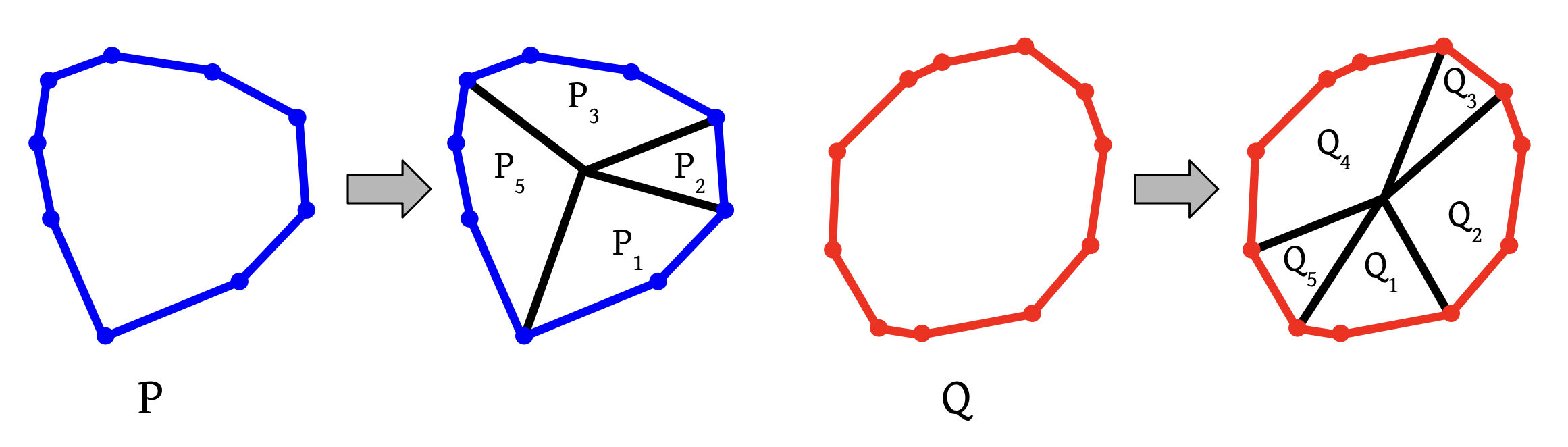
Given a parameter , referred to as the block size, we define a partition222Actually, it isn’t quite a partition because the boundaries may overlap, but these have zero area. of and into blocks and as follows. First (implicitly) sort the set333We assume that no angles are shared between the edges of and , as this case can be handled easily but requires a clumsier definition.
in increasing order and then partition the resulting sequence into consecutive subsequences of length each (except possibly the last one). We then define as the convex hull of the origin and the set of edges444The set of edges may be empty, in which case the block is just a single point (the origin). and . We define similarly. See Figure 1 for an example.
Now, uniquely defines the partition, so we refer to and as the blocks determined by parameter . This scheme is useful because the angle ranges and are strictly disjoint whenever , where is the set of edges that shares with , and is the set of edges that shares with . We call the restriction of ’s edges to , and similarly for .
3.1 A Data Structure Using Blocks
Towards producing a prune-and-search style algorithm, we want some way to reduce the time required to compute the vector which maximizes . Instead of reducing the complexity of or directly, we maintain and refine a specific data structure that contains information about and and allows us to rapidly search for optimal placements.
Definition 4 (-Block Structure).
A -block structure is a data structure containing the following:
-
1.
Access to the vertices of and in counterclockwise order with query time, and access to the area prefix sums for and with query time.
-
2.
A block size parameter , which implies blocks and .
-
3.
A region that is either (i) a triangle, (ii) a line segment, or (iii) a point.
-
4.
A partition of into subsets and , with the requirement .
-
5.
For every , access in time to a constant-complexity quadratic function such that for all .
Throughout, we assume that and are sorted, since we can apply radix sort in time . When using the block structure, we aim to decrease the size of while increasing the block size . If this is done carefully enough, we get a surprising result: a sublinear time oracle to report for any translation .
4 The Linear Time Algorithm
We will reduce Problem 1 to a few different subroutines/oracles. Roughly speaking, these allow us to produce a highly refined block structure in linear time, which can be used along with multidimensional parametric search [38] to find the translation of maximizing its area of intersection with in time .
Problem 2 (MaxRegion).
Given a -block structure for and , find
along with the translation realizing this maximum.555During some calls to MaxRegion, may not contain the global optimum.
Problem 3 (Cascade).
Given a -block structure, parameters and such that divides , and a triangle or line segment , either produce a -block structure, or report failure. Failure may be reported only if the interior of intersects more than lines from the set
| (2) |
where and are the blocks of and determined by .
The set may appear mysterious, but it simply corresponds to the line extensions for the edges that could “cause trouble” for the cascading procedure. The only observation necessary right now is that , i.e., is near-linear in size for all .
We write the expected time complexity of the fastest algorithm for MaxRegion as , where is the dimension of the region . We write the expected time complexity of the fastest algorithm for Cascade as . The latter will not depend on or the dimensions of and .
The next lemmas will be proved in Sections 5 and 6. The main idea behind proving each is to group most of the blocks of and into larger convex polygons that intersect in at most a constant number of locations, and then to process the rest via brute force.
Lemma 5 (Point Oracle).
For all , for all ,
Lemma 6 (Cascading Subroutine).
For all such that divides , for all ,
4.1 Reducing to the Point Oracle and Cascading Subroutine
We now give an algorithm for MaxRegion when the input -block structure has being a triangle or line segment. The algorithm works by invoking MaxRegion on regions with lower dimension to iteratively shrink .
Lemma 7.
For all such that divides , for all such that ,
Proof.
The algorithm for when is a line segment is nearly identical to the algorithm for when is a triangle, so for brevity we only focus on the triangle case. Let and be the blocks of and determined by block size parameter .
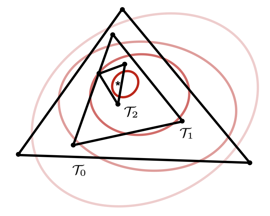
Define . We will produce a series of triangles such that each triangle is guaranteed to contain the optimal translation for the original region , and then take the final triangle in this sequence as . Once we have , we invoke Cascade to produce a -block structure, and then find the optimal translation within (along with the area for this translation) by invoking MaxRegion on this new block structure.
In the subsequent analysis, we show that, with high probability, the interior of produced as per our sequence will intersect at most lines of the set . If this event occurs, then Cascade will be forced to produce a -block structure. If this event does not occur, and Cascade returns failure, we can re-run the randomized algorithm to produce a new and try again. The expected number of attempts is , and so all of the steps (except for producing ) have a time overhead of .
Producing .
As per the above, the expected number of times we need to make is , so we only focus on the time complexity to make once. Consider producing a triangle from a triangle in the sequence. As a first step, we use Lemma 3 to make, with high probability, a -cutting for the lines of that intersect the interior of .
To apply this lemma, we need an efficient sampler. We argue that naive rejection sampling will suffice. Observe that if rejection sampling fails to find a random line of that intersects the interior of within time , then with high probability only lines of intersect . By assumption , so we can directly take . If rejection sampling is fast enough, then we can produce the required -cutting with high probability in time . Then, we intersect this cutting with and re-triangulate the resulting cells, which takes time in total.
The final step is to locate the cell of this triangulation that contains . This cell will be . To do this, we check all triangles by recursing in the dimension. We assume that is strictly contained within some cell, as the case that it is on the boundary can be detected similarly. Consider a single triangle . Let be an infinitesimally smaller copy of that is strictly inscribed within .666Infinitesimal shifts are a standard trick, and all of the algorithms in this paper can handle them without modification as long as they are implemented carefully enough. All bounding line segments for and are contained within . Therefore, we can use the input -block structure as a block structure for these line segments, and find the optimal translation (along with the area of intersection) restricted to each line segment in time . If one of the line segments for has a translation realizing a larger area than all of the line segments for , then by Lemma 1 we know that . Otherwise, does not contain .777All invocations might return a maximum area of zero, but we can handle this in time by checking whether an arbitrary translation that causes and to overlap is located within .
With high probability, the interior of will intersect at most half as many lines of as . By construction and the fact that divides (and hence ), we have . Thus there are at most iterations before we produce a triangle that intersects at most lines of with high probability and hence can be taken as . The time for all iterations is .
4.2 Putting it all Together
We now present our linear time algorithm. This amounts to solving a curious recurrence, and we actually have significant freedom in choosing the values for and .
Theorem 8.
There is an algorithm for Problem 1 running in expected time .
Proof.
We will always take and , so we can drop the and arguments from the time complexity of each subroutine/oracle. We begin by reducing from Problem 1 to an instance of MaxRegion over a -block structure, which requires no work beyond computing the area prefix sums because we can take and . Thus the total expected running time for Problem 1 will be .
Before analyzing , we find a closed-form expression for when . As per Lemmas 5, 6, and 7, we have the following for any such that divides :
We can efficiently parallelize the algorithm for zero-dimensional MaxRegion given in the proof of Lemma 5. So via a standard application of multidimensional parametric search (see Theorem 4.4 in the full version of [38]) that uses zero-dimensional MaxRegion for the decision problem, when for some constant . If we take (for example) and solve the recurrence, we get
Using the above along with Lemmas 5, 6, and 7, we have the following for any such that divides :
If we again take and stop to apply multidimensional parametric search when for some constant , we have recursion depth, and never exceeds . Solving the recurrence in the same way as for gives:
Clearly , and the theorem follows.
5 Constructing the Point Oracle
In this section, we prove the Point Oracle Lemma, restated below:
See 5
In other words, we need to use a given -block structure (where is just a single point ) to calculate . We can decompose the area function as
and then solve for each individual summation rapidly. The first summation is quite easy to compute by simply reading through the lists and that are provided.
Lemma 9.
There is an algorithm running in time such that, given a -block structure, where and consists of just a single point , it will compute
where and are the blocks of and determined by parameter .
Proof.
By definition of the block structure, we have a partition of into two subsets and such that , and for each we have a constant complexity quadratic function for all .
We can thus compute
in time by simply evaluating each . Since , we can compute
by evaluating the area for each directly. The time required is using known algorithms for intersecting two convex polygons whose edges are in sorted order.
We now turn our attention to the summation . Because every term amounts to computing the intersection for two blocks with different angle ranges, we could use binary searches to evaluate each term in time. However, this is too slow for our purposes, as there are a near quadratic number of terms. Instead, we take advantage of additional structure to decompose the summation into intersections of unions of blocks, such that each intersection can still be computed via binary search.
As a tool, we need a way to efficiently intersect convex chains that meet certain conditions.
Lemma 10.
Let and be any two convex polygons, and let and be any two polygonal chains whose edges are a subset of the edges of and , respectively. If , then and intersect at most twice, and we can find the intersection point(s) in time .
Proof.
Because the angle ranges for and are disjoint, they act as pseudo-disks, and hence can intersect at most twice. We can find the intersection point(s), if they exist, using a standard nested binary search in time (or a more clever binary search [37] in time, though we don’t need this improvement).
Now we can show how to compute .
Lemma 11.
There is an algorithm running in time such that, given a -block structure, where consists of just a single point , it will compute
where and are the blocks of and determined by parameter .
Proof.
We give a recursive algorithm for the problem. As a subroutine, we consider the problem of computing, given two integers with ,
Let be the time complexity of this subroutine. Since the original summation is equivalent to , the lemma amounts to showing that , or more generally, .
Consider an instance of this subroutine with any parameters . Let and . We can decompose the target summation as follows:
The first two summations can be evaluated in time at most via recursion (unless , in which case they are automatically zero). The last two summations can actually be evaluated directly. We consider the case of the very last summation; the remaining one can be evaluated via a symmetric process. First note that
Let and . Observe that and are both convex polygons, since each is the union of consecutive blocks. By construction, the edges that shares with and the edges that shares with form two convex polygonal chains that have disjoint angle ranges, i.e., . These chains account for all but two edges of and two edges of . Thus we can decompose and into convex polygonal chains satisfying the preconditions of Lemma 10. This implies that and intersect in at most a constant number of locations, and furthermore we can find the intersection points in time .
By decomposing and into pieces based on the intersection locations, we can use the area prefix sums888The area prefix sums for and also act as ares prefix sums for and ., along with a direct computation on the intersecting pairs of edges, to find the area of intersection in additional time. So the recurrence is when and . This solves to .
6 Constructing the Cascading Subroutine
The last step is to prove the Cascading Subroutine Lemma, restated below:
See 6
In other words, given a -block structure, parameters and , and a triangle or line segment , we want to either produce a valid -block structure, or report that more than lines of the set intersect . Throughout, let and be the blocks of and determined by block size parameter , and let and be the blocks of and determined by block size parameter .
First, we show that constant-complexity quadratic functions may actually be used to summarize the area function for certain block pairs.
Lemma 12.
Let and be any convex polygons, and let be any triangle or line segment contained in one cell of .999It is permissible for to touch the boundary of one cell, as long as it doesn’t strictly intersect. Then there exists a constant-complexity quadratic function such that for all .
Proof.
This follows from known observations by de Berg et al. [21].
Before describing how to perform cascading, we need a tool to help classify the new blocks based on their relationship with .
Lemma 13.
Let and be any two convex polygons, and let and be any two polygonal chains whose edges are a subset of the edges of and , respectively. Let be any triangle or line segment. If , then we can determine if some line segment in intersects the interior of in time .
Proof.
Let the set of vertices for be . For each , we know that, by Lemma 10, and can intersect in at most two points, and we can find the two pairs of edges that contain these intersection(s) in time .101010There is an edge case where at least one of the intersections occurs at a vertex of or a vertex of , but this can be handled with slightly more work without increasing the asymptotic running time. Let the set of all edge pairs for all vertices in be . We can determine if for all via brute force in time . If this is not the case, then some line segment of intersects the interior of , and we are done. If this is the case, then because is convex and each is convex, we have that each translation realizes a set of intersecting pairs that is a (possibly strict) superset of .
It remains to determine if any translations realize an intersecting pair not in , because this case (and only this case) would mean that a line segment in intersects the interior of . Let be with its edges participating in deleted, and let be with its edges participating in deleted. In time we can use techniques similar to the ones given above to determine if the interior of the (implicitly generated) Minkowski sum of and has any intersection with , and then if the interior of the (implicitly generated) Minkowski sum of and has any intersection with .
We are now ready to prove Lemma 6. The main observation is that the new quadratic functions stored in this data structure only need to apply when , not the more general case that , so many of the previously difficult blocks can now be handled. We will find a quadratic function for almost all indices in two steps:
-
1.
Scan through the information provided in the input -block structure, and use this to recover part of the function .
- 2.
Proof.
For all , note that because divides , we have a set of indices such that and .111111The set may be smaller for the very last value of , but this does not impact the proof. If for all and for all we can summarize with a constant-complexity quadratic function, then we can simply add these to get a new function .
We first argue that each quadratic function can be found efficiently, if it exists. Consider just a single value of . We use the decomposition
For the first summation on the right hand side, we scan through the list from the original -block structure. Each function with already has a quadratic function, and reading these takes time for each , or time for all . Globally, there are at most indices not in . For each of these, we can check whether lies in a single cell of via directly examining each line segment in in time . If this is the case, then by Lemma 12, can be summarized by a quadratic function for all , and we find the function via directly examining each parallelogram in in time ; the total additional time is . (If this fails for some , we will add the index to .)
Now consider the second summation on the right hand side. We can rewrite this as
where is the union of all ’s in the original sum with , and is the union of all ’s in the original sum with . We evaluate each of the terms individually.
Consider the case of , as the case of is symmetric. Now, is a convex polygon, because it is the union of consecutive blocks. By construction, . Therefore, we can break and into pieces that satisfy the preconditions of Lemma 10, showing that and can only intersect at a constant number of locations for any translation . These same pieces allow us to apply Lemma 13 to determine if lies in a single cell of , which takes time . If this is the case, then by Lemma 12 there exists a quadratic function equal to for all . The nonconstant components of this quadratic function only depend on the intersecting pairs of edges, and we have already found these via Lemma 13. Thus we can break and into pieces based on the intersection points, and use the area prefix sums from the -block structure (which also serve as area prefix sums for and ), to find the quadratic function equal to in additional time. (If this fails for some , we will add the index to .)
Adding the time across all terms for all gives an overall time of .
Each index for which we found a function is added to , and we store its function. The remaining indices are added to . The last step is to argue that , meaning we have constructed a valid -block structure.
By construction, note that every corresponds to an intersection between and the interior of . Also by construction (see Equation 2), each line in has at most two indices such is the line extension of some line segment in . Therefore we can charge each to different lines of in such a way that each line of will be charged at most twice. Thus if , this implies that more than lines of intersect the interior of , so the algorithm can just return failure in this case.
References
- [1] Pankaj K. Agarwal, Torben Hagerup, Rahul Ray, Micha Sharir, Michiel H. M. Smid, and Emo Welzl. Translating a planar object to maximize point containment. In Proc. 10th Annual European Symposium on Algorithms (ESA), volume 2461 of Lecture Notes in Computer Science, pages 42–53. Springer, 2002. doi:10.1007/3-540-45749-6_8.
- [2] Pankaj K. Agarwal and Micha Sharir. Efficient algorithms for geometric optimization. ACM Comput. Surv., 30(4):412–458, 1998. doi:10.1145/299917.299918.
- [3] Hee-Kap Ahn, Peter Brass, and Chan-Su Shin. Maximum overlap and minimum convex hull of two convex polyhedra under translations. Comput. Geom., 40(2):171–177, 2008. doi:10.1016/J.COMGEO.2007.08.001.
- [4] Hee-Kap Ahn, Siu-Wing Cheng, Hyuk Jun Kweon, and Juyoung Yon. Overlap of convex polytopes under rigid motion. Comput. Geom., 47(1):15–24, 2014. doi:10.1016/J.COMGEO.2013.08.001.
- [5] Hee-Kap Ahn, Siu-Wing Cheng, and Iris Reinbacher. Maximum overlap of convex polytopes under translation. Comput. Geom., 46(5):552–565, 2013. doi:10.1016/J.COMGEO.2011.11.003.
- [6] Hee-Kap Ahn, Otfried Cheong, Chong-Dae Park, Chan-Su Shin, and Antoine Vigneron. Maximizing the overlap of two planar convex sets under rigid motions. Comput. Geom., 37(1):3–15, 2007. doi:10.1016/J.COMGEO.2006.01.005.
- [7] Helmut Alt and Leonidas J. Guibas. Discrete geometric shapes: Matching, interpolation, and approximation. In Jörg-Rüdiger Sack and Jorge Urrutia, editors, Handbook of Computational Geometry, pages 121–153. North Holland / Elsevier, 2000. doi:10.1016/B978-044482537-7/50004-8.
- [8] Nancy M. Amato and Franco P. Preparata. A time-optimal parallel algorithm for three-dimensional convex hulls. Algorithmica, 14(2):169–182, 1995. doi:10.1007/BF01293667.
- [9] Gill Barequet, Matthew T. Dickerson, and Petru Pau. Translating a convex polygon to contain a maximum number of points. Comput. Geom., 8:167–179, 1997. doi:10.1016/S0925-7721(96)00011-9.
- [10] Sergio Cabello, Mark de Berg, Panos Giannopoulos, Christian Knauer, René van Oostrum, and Remco C. Veltkamp. Maximizing the area of overlap of two unions of disks under rigid motion. Int. J. Comput. Geom. Appl., 19(6):533–556, 2009. doi:10.1142/S0218195909003118.
- [11] Timothy M. Chan. A simpler linear-time algorithm for intersecting two convex polyhedra in three dimensions. Discret. Comput. Geom., 56(4):860–865, 2016. doi:10.1007/S00454-016-9785-3.
- [12] Timothy M. Chan. (Near-)linear-time randomized algorithms for row minima in Monge partial matrices and related problems. In Proc. of the 32nd ACM-SIAM Symposium on Discrete Algorithms (SODA), pages 1465–1482, 2021. doi:10.1137/1.9781611976465.88.
- [13] Timothy M. Chan and Isaac M. Hair. Convex polygon containment: Improving quadratic to near linear time. In Proc. 40th International Symposium on Computational Geometry (SoCG), volume 293 of LIPIcs, pages 34:1–34:15, 2024. doi:10.4230/LIPICS.SOCG.2024.34.
- [14] Bernard Chazelle. The polygon containment problem. Advances in Computing Research, 1(1):1–33, 1983. URL: https://www.cs.princeton.edu/˜chazelle/pubs/PolygContainmentProb.pdf.
- [15] Bernard Chazelle. Triangulating a simple polygon in linear time. Discret. Comput. Geom., 6:485–524, 1991. doi:10.1007/BF02574703.
- [16] Bernard Chazelle. Cuttings. In Dinesh P. Mehta and Sartaj Sahni, editors, Handbook of Data Structures and Applications. Chapman and Hall/CRC, 2004. doi:10.1201/9781420035179.CH25.
- [17] Bernard Chazelle and Leonidas J. Guibas. Fractional cascading: I. A data structuring technique. Algorithmica, 1(2):133–162, 1986. doi:10.1007/BF01840440.
- [18] Siu-Wing Cheng and Chi-Kit Lam. Shape matching under rigid motion. Comput. Geom., 46(6):591–603, 2013. doi:10.1016/J.COMGEO.2013.01.002.
- [19] Kenneth L. Clarkson. New applications of random sampling in computational geometry. Discret. Comput. Geom., 2:195–222, 1987. doi:10.1007/BF02187879.
- [20] Kenneth L. Clarkson and Peter W. Shor. Application of random sampling in computational geometry, II. Discret. Comput. Geom., 4:387–421, 1989. doi:10.1007/BF02187740.
- [21] Mark de Berg, Otfried Cheong, Olivier Devillers, Marc J. van Kreveld, and Monique Teillaud. Computing the maximum overlap of two convex polygons under translations. Theory Comput. Syst., 31(5):613–628, 1998. doi:10.1007/PL00005845.
- [22] Martin E. Dyer. Linear time algorithms for two- and three-variable linear programs. SIAM J. Comput., 13(1):31–45, 1984. doi:10.1137/0213003.
- [23] Martin E. Dyer. On a multidimensional search technique and its application to the euclidean one-centre problem. SIAM J. Comput., 15(3):725–738, 1986. doi:10.1137/0215052.
- [24] Greg N. Frederickson and Donald B. Johnson. Generalized selection and ranking: Sorted matrices. SIAM J. Comput., 13(1):14–30, 1984. doi:10.1137/0213002.
- [25] Sariel Har-Peled and Subhro Roy. Approximating the maximum overlap of polygons under translation. Algorithmica, 78(1):147–165, 2017. doi:10.1007/S00453-016-0152-9.
- [26] Shreesh Jadhav and Asish Mukhopadhyay. Computing a centerpoint of a finite planar set of points in linear time. Discret. Comput. Geom., 12:291–312, 1994. doi:10.1007/BF02574382.
- [27] Mook Kwon Jung, Seokyun Kang, and Hee-Kap Ahn. Minimum convex hull and maximum overlap of two convex polytopes. In Proc. 36th ACM-SIAM Symposium on Discrete Algorithms (SODA), 2025. To appear.
- [28] Garam Kim, Jongmin Choi, and Hee-Kap Ahn. Maximum overlap of two convex polygons. KIISE Transactions on Computing Practices, 27(8):400–405, 2021. doi:10.5626/KTCP.2021.27.8.400.
- [29] Jirí Matoušek. Approximations and optimal geometric divide-an-conquer. J. Comput. Syst. Sci., 50(2):203–208, 1995. doi:10.1006/JCSS.1995.1018.
- [30] Nimrod Megiddo. Applying parallel computation algorithms in the design of serial algorithms. J. ACM, 30(4):852–865, 1983. doi:10.1145/2157.322410.
- [31] Nimrod Megiddo. Linear-time algorithms for linear programming in and related problems. SIAM J. Comput., 12(4):759–776, 1983. doi:10.1137/0212052.
- [32] Nimrod Megiddo. Linear programming in linear time when the dimension is fixed. J. ACM, 31(1):114–127, 1984. doi:10.1145/2422.322418.
- [33] Nimrod Megiddo. Partitioning with two lines in the plane. J. Algorithms, 6(3):430–433, 1985. doi:10.1016/0196-6774(85)90011-2.
- [34] David M. Mount, Ruth Silverman, and Angela Y. Wu. On the area of overlap of translated polygons. Comput. Vis. Image Underst., 64(1):53–61, 1996. doi:10.1006/CVIU.1996.0045.
- [35] Wlodzimierz Ogryczak and Arie Tamir. Minimizing the sum of the largest functions in linear time. Inf. Process. Lett., 85(3):117–122, 2003. doi:10.1016/S0020-0190(02)00370-8.
- [36] Joseph O’Rourke, Subhash Suri, and Csaba D. Tóth. Polygons. In Jacob E. Goodman, Joseph O’Rourke, and Csaba D. Tóth, editors, Handbook of Discrete and Computational Geometry, pages 787–810. Chapman and Hall/CRC, 3rd edition, 2017. URL: https://www.csun.edu/˜ctoth/Handbook/chap30.pdf.
- [37] Mark H. Overmars and Jan van Leeuwen. Maintenance of configurations in the plane. J. Comput. Syst. Sci., 23(2):166–204, 1981. doi:10.1016/0022-0000(81)90012-X.
- [38] Sivan Toledo. Maximizing non-linear concave functions in fixed dimension. In Proc. 33rd Annual Symposium on Foundations of Computer Science (FOCS), pages 676–685, 1992. doi:10.1109/SFCS.1992.267783.
- [39] Eitan Zemel. An algorithm for the linear multiple choice knapsack problem and related problems. Inf. Process. Lett., 18(3):123–128, 1984. doi:10.1016/0020-0190(84)90014-0.
- [40] Honglin Zhu and Hyuk Jun Kweon. Maximum overlap area of a convex polyhedron and a convex polygon under translation. In Proc. 39th International Symposium on Computational Geometry (SoCG), volume 258 of LIPIcs, pages 61:1–61:16, 2023. doi:10.4230/LIPICS.SOCG.2023.61.