A Theory of Sub-Barcodes

Abstract
The primary tool in topological data analysis (TDA) is persistent homology, which involves computing a barcode – often from point-cloud or scalar field data – that serves as a topological signature for the underlying function. In this work, we introduce sub-barcodes and show how they arise naturally from factorizations of persistence module homomorphisms. We show that, as a partial order induced by factorizations, the relation of being a sub-barcode is strictly stronger than the rank invariant, and we apply sub-barcode theory to the problem of inferring information about the barcode of an unknown Lipschitz function from samples. The advantage of this approach is that it permits strong guarantees – with no noise – while requiring no sampling assumptions, and the resulting barcode is guaranteed to be a sub-barcode of every Lipschitz function that agrees with the data. We also present an algorithmic theory that allows for the efficient approximation of sub-barcodes using filtered Delaunay triangulations for Euclidean inputs.
Keywords and phrases:
Topology, Topological Data Analysis, Persistent Homology, Persistence Modules, Barcodes, Sub-barcodes, Factorizations, Lipschitz ExtensionsCopyright and License:
2012 ACM Subject Classification:
Mathematics of computing Algebraic topology ; Mathematics of computing Geometric topology ; Theory of computation Computational geometry ; Computing methodologies Algebraic algorithmsFunding:
This work was partially funded by the NSF under grant CCF-2017980.Editors:
Oswin Aichholzer and Haitao WangSeries and Publisher:
1 Introduction
Topological data analysis (TDA) seeks to compute topological properties of unknown functions from finite samples. The most widely-used tool for TDA is persistent homology (PH), and the most widely-studied functions are distance functions. Thus, the algorithmic problems arising in this field tend to be either algebraic (PH computation), geometric (distance function representation), or both.
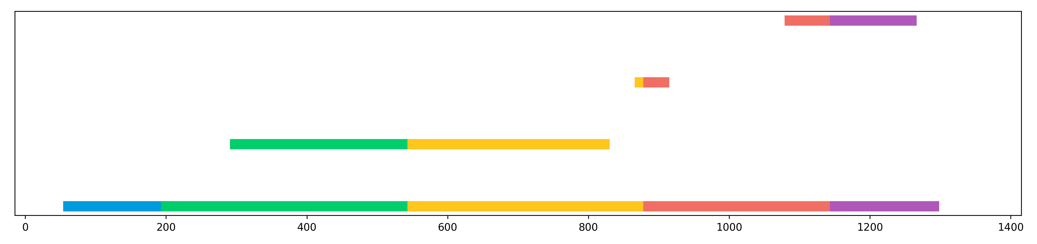
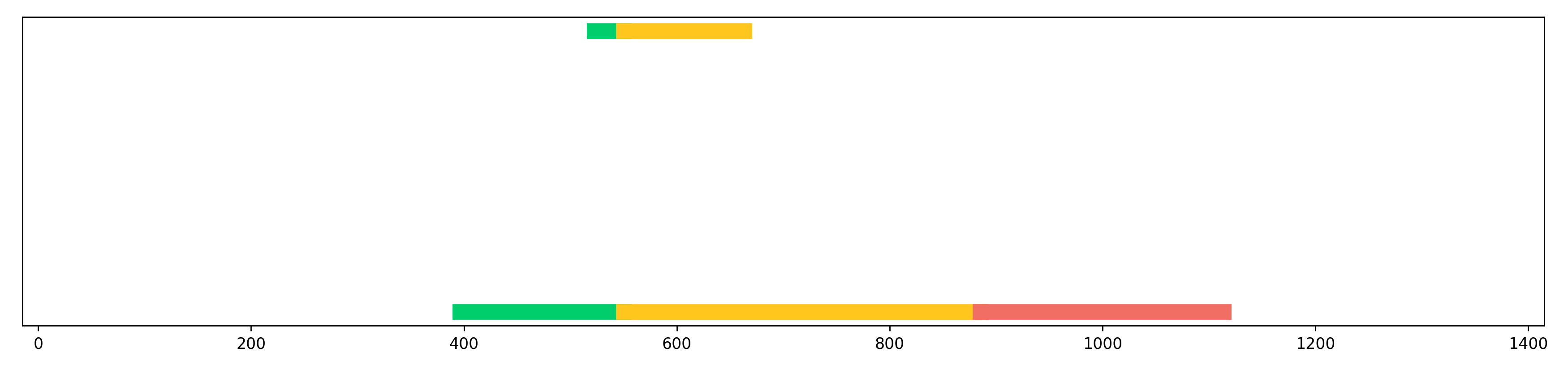
A PH pipeline starts with a real-valued function as input, and then considers the sublevel sets of this function. The homology of the sublevels at each threshold value are tracked and aggregated into a barcode (see Figure 1). The goal is to compute or approximate this barcode, which often requires substantial assumptions on the quality of the sample.
In this paper, we relax this goal to instead compute whatever sub-barcode is supported by the data we have. We form a sub-barcode by taking a sub-interval of each bar in the barcode. The formal definition of a sub-barcode and how it arises naturally in PH is covered in Section 3. The main idea is that, given some of the data, we compute some of the underlying structure.

In practice, analyzing the topology of a finite sample entails two main challenges:
-
Extension: If is a finite sample of the underlying space , then we need to extrapolate the values for a function from the known values at to the unknown values at the rest of . We won’t get the exact answer, but we would like some guarantees on the extension.
-
Discretization: Having a good approximation to the function is insufficient: we also need a reliable discrete representation of the underlying space. In practice, these representations usually arise in the form of a simplicial complex or a simplicial set.
In the classic setting of distance functions in Euclidean space, strong sampling assumptions guarantee that the distance to a sample approximates the distance to the underlying set. The Delaunay triangulation provides a perfect discretization, capturing the exact homology of the distance sublevels. This was the original setting for PH [13].
Lipschitz functions generalize distance functions and allow us to represent a much wider class of inputs. Several previous papers have shown that, given a sufficiently dense sample, a good approximation to the barcode of a Lipschitz function can be computed [6, 8, 11]. The guarantees from such work is that the output barcode is close to the true barcode in a standard metric called the bottleneck distance. Our approach eliminates all sampling assumptions, but gives guarantees in terms of a partial order on barcodes; that is, it is guaranteed to produce no noise or spurious bars, but finds only those topological features (bars) that are sufficiently supported by the sample.
Contributions and Outline
The background and definitions appear in sections 2 and 3. The algebraic theory of sub-barcodes is presented in Section 4. First, we show how sub-barcodes are related to the widely-studied rank invariant. Surprisingly, despite being a complete invariant for persistence, the natural extension of the rank invariant to a partial order is strictly less discriminating than sub-barcodes. This would be useless if it were not the case that sub-barcodes can be computed, a fact we show in the main sub-barcode theorem (Theorem 4), which states that sub-barcodes arise whenever we have one persistence module homomorphism factoring through another.
In Section 5, we lay out the extension theory. According to the algebraic theory of the previous section, the key to producing sub-barcodes is to find suitable upper and lower bounds on the unknown function. We show that maximum and minimum Lipschitz extensions serve this purpose (Figure 2), as well as how to give good guarantees with only an approximation to the upper and lower bounds (Corollary 9). This section also contains a much more general result to encompass other classes of functions beyond Lipschitz functions (Theorem 11).
The discretization theory is presented in Section 6. Here, we show how to approximate the Lipschitz extension sub-barcode of the previous section using Delaunay triangulations. This leads to a theory of semi-supervised TDA in which only a subset of function values are known (Theorem 13). We also give a tighter approximation using the barycentric decomposition of the Delaunay triangulation (Theorem 14), and show that this method also applies to a wider class of functions (Example 15).
The categorical theory of sub-barcodes is presented in Section 7. The TDA and PH pipeline depend on category theory to express the way relationships between inputs impact relationships between outputs, i.e., barcodes. We relate sub-barcodes to the classic approach of smoothing barcodes and show how this arises naturally from categorical considerations. We also give a new perspective on barcodes in general for which sub-barcodes are shown to be true subobjects in the categorical sense, and discuss how this construction is related to the theory of fuzzy sets [15, 1, 21].
2 Background
Functions and Filtrations
Let be a metric space. When the metric is Euclidean, we denote the distance as a norm, i.e., . The distance from a point to a (finite) set is denoted .
The real-valued functions form a vector space where , for all . We also have a poset of functions, where iff for all . A function is -Lipschitz if, for all , we have
If is not specified, then it is assumed that . This is perhaps not the most common way to express the Lipschitz condition, but it is closest to how it is used in this work.
The -sublevel set of is the set of points with :
This notation is designed to indicate that is a filtration: for we have . There is a partial order on sublevel filtrations where iff for all . It is a simple exercise to check that, if , then ; i.e., larger functions have smaller sublevel sets.
Remark 1.
The mapping from a function to its sublevel filtration is a contravariant functor from the poset of functions to the poset of filtrations. The filtrations themselves are functors from the totally ordered set of real numbers to , the category of topological spaces. Throughout, we use remarks like this one to highlight the categorical interpretations. The reader who is unfamiliar with these terms may still follow all definitions and algorithms.
Persistence Modules
A pointwise finite dimensional (p.f.d.) persistence module assigns a (finite-dimensional) vector space to all and a linear map for all . The map is the identity on , and for all , . For persistence modules and , a homomorphism assigns linear maps for all so that for all , we have .
Remark 2.
A persistence module is a functor , and a persistence module homomorphism is a natural transformation between functors , so that the category of persistence modules is precisely the category of functors .
A factorization of homomorphisms to is given by a pair of homomorphisms such that (Diagram 1).
| (1) |
Let denote the category with homomorphisms of persistence modules as objects, and arrows . Then is a factorization of through .
Example 3.
Letting denote a persistence module shifted by a constant , a -interleaving is traditionally given by a pair of commuting diagrams
| (2) |
| (3) |
Homology
Homology is a topological invariant that is particularily useful because it is both informative and efficiently computable for triangulable topological spaces. A homology functor associates a vector space to a topological space , and takes continuous maps between topological spaces to linear maps between the corresponding vector spaces.
Persistence modules naturally arise in TDA by taking the homology of a sublevel filtration of a function. This assembles the functorial TDA pipeline from functions to filtrations to persistence modules. It is useful to see these as functors and not just functions because the additional structure of functoriality tells us that, if , then there is a persistence module homomorphism . As we will see, these homomorphisms can be combined into factorizations (leading to sub-barcodes) and interleavings (leading to approximations).

3 Barcodes and Sub-Barcodes
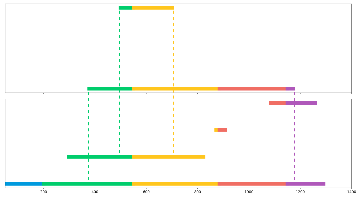
Let denote the poset of intervals on ordered by inclusion. A barcode is a function where is a set whose elements are called bars. The barcode assigns an interval to each bar. Note that is not necessarily injective. When there is no confusion, we identify the bars in a barcode with their corresponding intervals. A sub-barcode mapping between barcodes and is a function such that, for all , we have . If is injective, then we call it a sub-barcode matching and say is a sub-barcode of , denoted . That is, is a sub-barcode of if can be formed from by taking a subinterval of each bar in a subset of (Figure 4).
There is a barcode corresponding to any persistence module . Note, the image of a persistence module homomorphism is also persistence module. We overload notation and write to indicate .
From the PH pipeline, we have persistence modules associated with each continuous function . We again simplify our notation and write to denote and to denote . The object giving us a barcode is always clear from context.
We now have enough definitions to state the main theorem of sub-barcodes. The proof is postponed until Section 4 when we will have developed some necessary tools.
Theorem 4 (The Sub-Barcode Theorem).
If there exists a factorization of persistence module homomorphisms (i.e., ), then .
4 The Algebraic Theory
4.1 Sub-barcodes vs. Ranks
Let denote the rank of a linear map defined as the dimension of its image, . The rank invariant of a persistence module is a function from ordered pairs in to the natural numbers defined as . It is straightforward to extend this invariant to homomorphisms by letting . In the following, we consider the rank invariant for a persistence module to be the rank invariant of its identity homomorphism, i.e., .
A basic fact from linear algebra is that, if a linear map factors through a second linear map , then . It follows immediately that, if there is a factorization of persistence module homomorphisms, then for all ,
This puts a partial order on rank invariants that we call the sub-rank relation and denote by .
Remark 5.
is a contravariant functor and is a contravariant functor , i.e., from factorizations of vector spaces (resp. persistence modules) to the poset of natural numbers. An ordering of two rank invariants is a natural transformation between these functors.
In light of the sub-barcode theorem, the rank invariant is the same type of invariant as sub-barcodes. It puts a partial order on morphisms induced by factorizations. However, although the barcode can be constructed from the rank invariant, the natural ordering of rank invariants is a weaker invariant than sub-barcodes as expressed in the following.
Theorem 6.
The sub-barcode order is a more discriminating invariant than the sub-rank order in the sense that, for all persistence module homomorphisms and , implies that , but not vice-versa.
Proof.
The rank invariant is easily extracted from a barcode: is the number of bars in that contain the closed interval . It follows immediately from the injectivity of the sub-barcode matching (and the pigeonhole principle) that implies that .
For the other side of the proof, it suffices to give an example of persistence modules and such that while .111As before, is shorthand for . Let be a persistence module where has two bars corresponding to intervals and , and let be a persistence module such that has only one bar corresponding to the interval . Clearly, , but it is not possible for a barcode with two bars to be a sub-barcode of one with only one bar. Thus .
4.2 Induced Matching Theory Proof of the Sub-Barcode Theorem
Although not expressed in these terms, Bauer and Lesnick’s theory of induced matchings [3] shows that sub-barcode matchings arise from certain homomorphisms. The induced matchings in that work are matchings between the bars that do not (necessarily) satisfy the inclusion requirement of a sub-barcode matching. They showed that for any homomorphism , there is a partial bijective function (a matching) between the bars with the property that every bar of is the intersection of the intervals of the matched bars from to . These are constructed from the pair of canonical (functorial) matchings induced by the epi-mono factorization of through its image. Translated into the vocabulary of sub-barcodes, this result implies that and .
More generally, if is a monomorphism (all maps are injective), then . This is because the induced matching of a monomorphism matches every bar, in addition to the property that, if is matched to , then and ; thus, a submodule relation between persistence modules implies a sub-barcode relation between the barcodes.
If is an epimorphism (all maps are surjective), then the induced matching is surjective, and if is matched to , then and . So, reversing this induced matching, we get . We use these matchings in the proof of the Sub-Barcode Theorem below.
Proof of The Sub-Barcode Theorem (Theorem 4).
The factorization entails . Let be the unique monomorphism given by the universal property of images, and let be the epimorphism given by resticting to . Using the induced matching theory, gives a sub-barcode matching . Then, the reverse of the matching induced by gives a sub-barcode matching . Putting these together, we get
The following corollary for ordered sequences of functions forms the basis for all of our applications of sub-barcodes in TDA.
Corollary 7.
If are functions , then .
Proof.
It suffices to observe that the ordering on the functions gives a factorization of through . By the functoriality of the sublevel functor and homology, we get the corresponding factorization of persistence modules. The claim then follows from Theorem 4.
5 The Extension Theory
Given an unknown Lipschitz function and a sample , let denote the function restricted to the points of . The pair denotes input to a TDA problem where the goal is to infer as much as possible about . Any function that agrees with at the points of is called an extension of . If is also Lipschitz, then it is called a Lipschitz extension. By the definition of Lipschitz continuity, each point puts an upper bound and a lower bound on the unknown so that
The combination of these upper and lower bounds gives the maximum and minimum Lipschitz extensions, defined respectively for each as
Note that the max extension is the minimum of the upper bounds and vice versa (see also [17]).
The following theorem states that, for every Lipschitz function that agrees with the data, the max and min Lipschitz extensions yield a barcode that is contained in .
Theorem 8.
Given and , for all Lipschitz extensions of , we have .
Proof.
It suffices to observe that for all Lipschitz extensions of , we have . Because , the result follows from Corollary 7.
The Choice of Lipschitz Constants
It is natural to ask whether (and how) the choice of the Lipschitz constant affects this result. The previous statements have all assumed -Lipschitz functions. More generally, tuning the Lipschitz constant naturally leads to a filtration of the barcode itself as shown in the following.
Corollary 9.
For any , let and denote the (resp.) max and min -Lipschitz extensions. If is -Lipschitz and , then .
A Sub-Barcode that is Close in Bottleneck Distance
A fundamental challenge in computing sub-barcodes from Lipschitz extensions is that it is not clear how to construct a simplicial complex that can represent the sublevel sets of both the max and min extension at the same time. So, in order to still derive guarantees, it will suffice to have approximations to these extensions. The following theorem shows that a bottleneck-close sub-barcode is possible if we have close approximations to the upper and lower bounds.
Theorem 10.
Let be an ordered sequence of functions such that and . Then, .
Proof.
The proof is a straightforward application of the general stability theorem for image persistence. The bounds and imply that and . As all maps from ordered functions induce inclusions of sublevel sets, all required maps commute to form an interleaving in the arrow category of filtrations. This gives an interleaving in the arrow category of persistence modules which leads to an -interleaving of the image persistence modules.
Beyond Lipschitz Functions
The careful reader may note that there is nothing particularly special about Lipschitz functions in the treatment above. One could consider other classes of functions as well. More generally, it suffices to have an upper and lower bound on the unknown function. In the Lipschitz case, the Lipschitz extensions form a lattice of hypotheses that we are considering. Recall that a poset is a lattice if every subset has a join (least upper bound) and a meet (greatest lower bound). The symbol is used for joins and is used for meets. This is the origin of our notation and .
For a set of functions, let and . In particular, if denotes the set of Lipschitz extensions of , then and . For other lattices of hypotheses, the same proof as for the Lipschitz case (Theorem 8) implies the following theorem.
Theorem 11.
Given a lattice of functions , for all , we have
6 The Discretization Theory
The preceding sections laid out the theory of sub-barcodes for persistence modules, as well a the useful setting of Lipschitz functions. The following section shows how to approximate these barcodes.
The fundamental challenge is to provide a single discretization of space that approximates (or at least bounds) both Lipschitz extensions at the same time. We assume throughout this section that is a convex polytope in .222The convexity of can be relaxed in many settings. Assuming is convex simplifies our use of the Nerve theorem. For a finite set , the Voronoi diagram assigns a convex polytope called the Voronoi cell to each point defined as
The radius of is the maximum distance from to any point in the cell: . More generally, for , we have a Voronoi cell
Dually, the Delaunay triangulation associated with is the simplicial complex with vertex set and simplices . The Delaunay triangulation is widely used for persistent homology on Euclidean inputs.
6.1 Simple Voronoi Extensions and a Delaunay Filtration
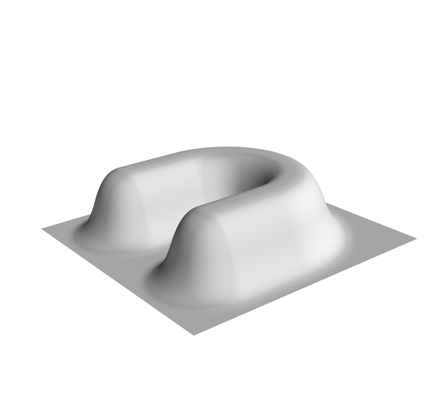
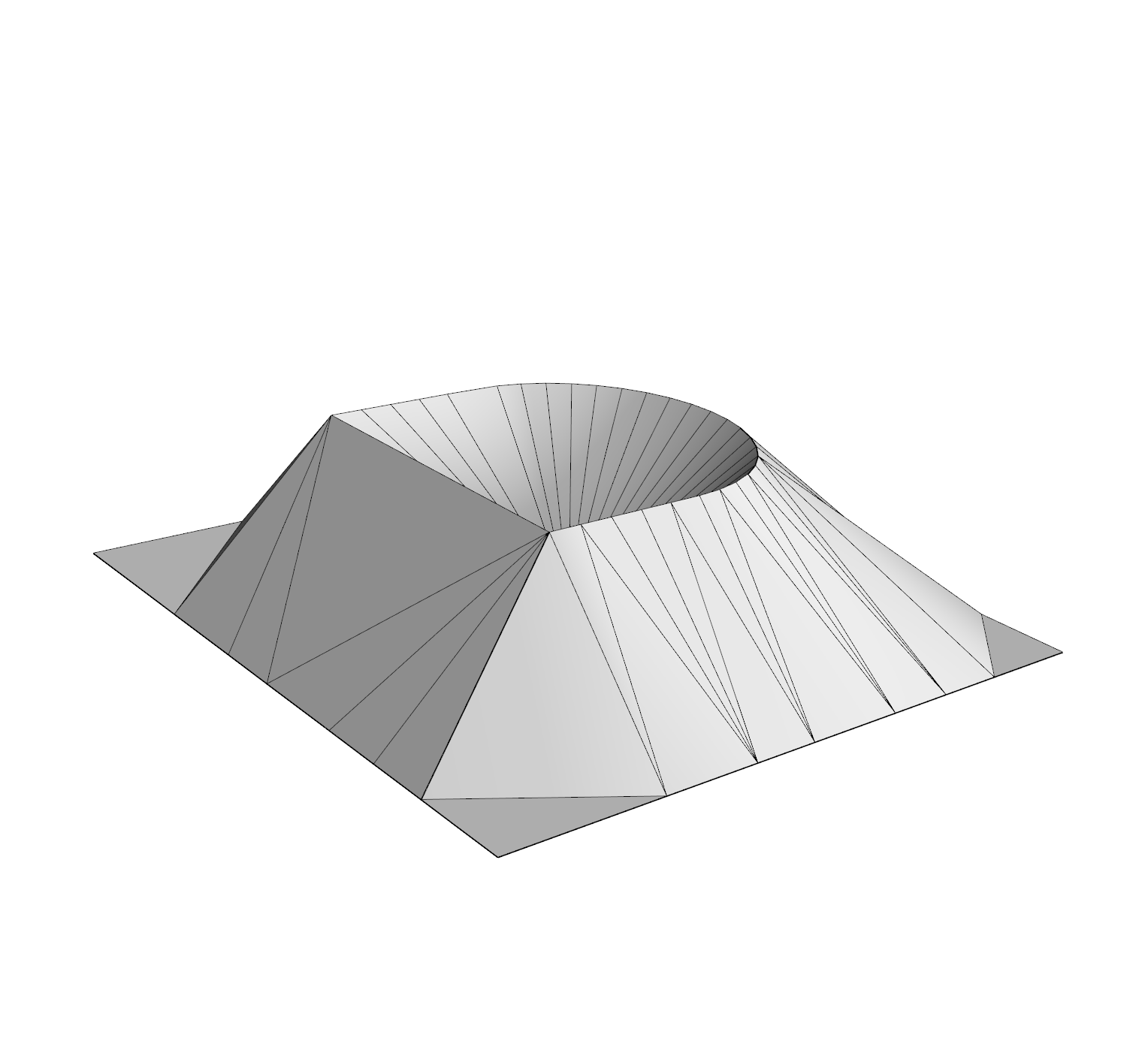
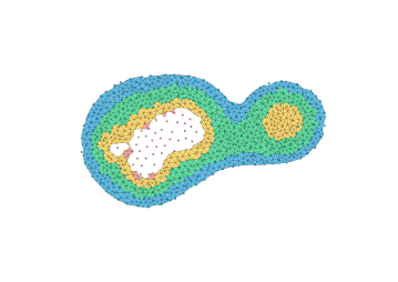
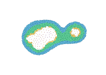
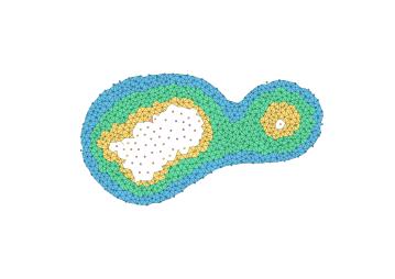
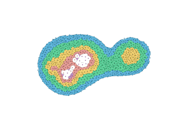
The most direct way to use a Delaunay triangulation to estimate the persistence diagram of a set of points is to extend the function from the vertex set to the simplices, setting the value at the simplex be the maximum value at its vertices. This corresponds to the piecewise linear extension of the function to the geometric realization of the complex (see Section 2.5, Morozov [20]). Unfortunately, this can fail badly in the absence of strong sampling guarantees; Figure 5 shows an example where the piecewise linear extension introduces spurious features. Thus, the problem with some samples is not only that we can miss features, but that we may hallucinate them as well.
The key to using a discretization is to use an image filtration (see Cohen-Steiner et al. [12], Bauer [4]) capturing both an upper and lower bound. The following theorem states that we can compute a sub-barcode for any Lipschitz function by filtering the Delaunay triangulation by upper and lower bounds given on the input values and the radius of the Voronoi cells.
Theorem 12.
Let be a finite subset of a polytope . Let be a sample of an unknown Lipschitz function . For each , let denote the radius of the Voronoi cell . Let and be functions defined on Delaunay simplices as
Then, .
Proof.
To relate the barcodes, we will first construct functions on that have the same barcode as the simplicial functions and . Second, we will relate these functions to the Lipschitz extensions and .
We define piecewise constant functions on using the Voronoi cells and as
By the Persistent Nerve Lemma (Chazal et al. [9], Lemma 3.4), there is a homotopy equivalence between the sublevels of and that commutes with inclusions (see also [2]). The same holds for and . It follows that .
For any , there is an such that and , so
Similarly, there is an such that and , so
thus , and Corollary 7 therefore implies
6.2 Semi-Supervised TDA
We have assumed thus far that we have access to function values at all points in the sample. This resembles a supervised learning problem. If instead we only have function values at a subset , we can still use the points of to improve our approximation. We call this semi-supervised TDA.
The most common guarantees in PH are derived from interleavings, and thus yield bottleneck distance bounds on the resulting barcodes. In this section, we combine those results with the Lipschitz extension sub-barcode and the Delaunay filtration above to get a guaranteed approximation. Throughout, we assume that is a sample of , and that we only have function values for . The algorithm extends and to the points of and then use the Delaunay filtration from the previous subsection.
In the following, we say that is an -sample of if every point of is within of a point in . Equivalently, the radius of every Voronoi cell is at most .
Theorem 13.
Let be a convex polytope, and suppose is an -sample. Let be a sample of an unknown Lipschitz function defined on a subset , and let and be functions defined on each Delaunay simplex as
Then, , and .
Proof.
The sub-barcode relation follows from Theorem 12 and the observation that the radius for all in an -sample. The bottleneck bound follows from a more general theory of interleaving of image persitence modules. It depends only on the fact that the extensions and of and to piecewise constant functions on Voronoi cells (as in the proof of Theorem 12) satisfy and , respectively. These bounds yeild an -interleaving of the sublevels, and thus give an interleaving of the images.333A more general theorem for stabilty of image persistence can be found in the full version of this paper [10].
6.3 Finer Approximation with Barycentric Subdivision
In general, we would like to have tight approximations to the sub-barcode of Lipschitz extensions without requiring any sampling assumptions. One way to get a better bound is to manually add points to reduce the radii of the cells. Another approach would be to consider the barycentric subdivision. This makes sense because it can be understood as assigning function values to Delaunay simplices individually rather than inducing the values from the function on the vertices. In this section, we show how to define such constructions in a way that applies to a much more general class of functions.
For each sample , knowing the value of implies an upper bound and a lower bound on . Thus far, these bounds came from the assumption that is Lipschitz. Similar upper and lower bounds can be defined for other classes of functions. We only assume that these bounds are distance monotone. That is, the upper bound for a point satisfies the condition that if , then . For the lower bound at values decrease with distance, i.e., if , then . We call and a family of pointwise distance monotone bounds. As before, we let and .
Although the term baryentric subdivision implies that subdivision happen at the barycenters of the cells, we define this operation instead as a combinatorial operation on simplicial complexes. For any simplicial complex , we define to be the simplicial complex with a vertex for each simplex in and a simplex for each ordered subset of simplices (the ordering is by inclusion). For any function , we can extend it to a filtration on , as is in if and only if for all . Proof of the following theorem may be found in the full version [10].
Theorem 14.
Let be a finite sample of a convex polytope , and let and be families of pointwise distance-monotone bounds on some unknown function . Aggregate these bounds as and . For , let
Extend and to . Then, .
Example 15.
To apply this theorem to the special case of Lipschitz functions, the resulting filtration captures the usual Lipschitz upper and lower bounds restricted to the Voronoi cells. That is,
Letting be the birth time of the simplex in the standard Delaunay filtration (also known as the -complex filtration). Then, the corresponding filtration on is induced by
7 Categorical Constructions
The following section describes how the concepts presented above fit neatly into a category-theoretic framework. It contains some technical concepts that may unfamiliar to computational geometers.
7.1 Smoothing Persistence Modules
Given a barcode , an -smoothing is a new barcode defined by eliminating bars of length at most , and replacing all other bars with a ; that is, we trim from the beginning and the end of each bar. The idea of a smoothed barcode naturally arises in the literature on the stability of persistence modules [7, 5, 18]. It is clear from the definition that the smoothed barcode is a sub-barcode of the original. This relationship can be expressed clearly as arising from a factorization as follows.
Let and be order-preserving maps with the property that, for all , we have . Order preserving maps between posets are functors, so the pointwise order relations on and correspond to natural transformations
So, for any persistence module , composition with yields the following factorization.
| (4) |
Letting , we can view (or equivalently, its image) as the smoothed persistence module. The factorization induces the sub-barcode matching in the obvious way:
From this perspective, an interleaving of persistence modules may be viewed as a pair of compatible factorizations rather than a pair of compatible (shifted) homomorphisms. In fact, the pair corresponds to an adjunction with counit and unit (see [14]).
7.2 Sub-Barcodes are Subobjects
Within the literature, there are several different categorifications of persistence barcodes (or equivalently persistence diagrams). Here, we identify a natural way to define a category of barcodes that plays nicely with our treatment of sub-barcodes.
First, recall that unlike much of the prior work, we do not regard barcodes as multisets. Instead, we define a barcode to be a function from a set to the intervals. In computer programming terms, we have an “is a” versus “has a” distinction; in the multiset view, each bar is an interval. In our view, each bar has an interval.
A standard categorical approach to construct a category from a (pseudo)functor is the Grothendieck construction. Let be a functor from a category to the category of (small) categories. For the purposes of this work, the (covariant) Grothendieck construction yields a category with objects given by pairs for each and , and arrows for each pair of arrows in and in .
Let be the (pseudo)functor that takes a set and returns the category of functors . Then the category of barcodes described in Section 3 is a contravariant Grothendieck construction
The objects of are pairs – i.e. barcodes – and a morphism of is a function such that for all , we have that . To see this as a Grothendieck construction, it suffices to observe that the barwise inclusion ordering is a natural transformation in .
The condition on morphisms ensures that a bar can only map to a bar when . Thus, a injective morphism is exactly a sub-barcode matching. These injective morphisms are the monomorphsisms in this category and thus sub-barcodes are subobjects in this category.
Remark 16.
The category defined above is also known as the category of -fuzzy sets [15], and the construction of a category of fuzzy sets using the Grothendieck construction also noted by Jardine [16]. It is also possible to replace with , the category of sets with partial injective maps (i.e., matchings), to construct barcodes as , or more generally, to replace with the category of sets and partial functions. In both cases, the monomorphisms are injective sub-barcode matchings that yield sub-barcode relations.
7.3 Ranks via Presheaves
The rank functor was previously constructed directly from a persistence module, or more generally, a factorization of persistence module homomorphisms. In this section, we show how the rank functor can also be constructed from a barcode. This is already well-known; the novelty here is that we show how the rank functor can be factored through the category of barcodes. This gives the more abstract proof that sub-barcodes are more discriminating than ranks.
For any category , there is a functor given for by
The morphisms are inclusions . For in , it is easy to check that gives a natural transformation .
For the special case where , this is a functor from barcodes to presheaves of intervals. The intuitive meaning is that, for a barcode , the presheaf maps an interval to the set of bars in that contain all of . All morphisms in the image of are inclusions, and so, for , we have and thus . Here the vertical bars indicate set cardinality which is a functor from the poset of finite sets with inclusions to the poset . Thus, we have a functor .
It is now an easy exercise to show that . All morphisms in the functor category are monomorphisms, so clearly a sub-barcode relation (a monomorphism of barcodes) yields a subrank relation (a monomorphism of rank invariants). The other direction doesn’t hold. The most natural way to define a barcode from the rank invariant does not give a functor to barcodes. The example is given in the proof of Theorem 6.
Remark 17.
Barr [1] showed that, when the indexing poset is a Heyting algebra, the category of -fuzzy sets is equivalent to a category of sheaves of monomorphisms. Following this result, many of the recent applications of fuzzy sets [21, 19] have defined fuzzy sets directly as functors . Unfortunately, because the poset of intervals is not a Heyting algebra, this equivalence cannot be applied directly to the category . On the other hand, the category of intervals with the product or Egli-Milner ordering is a Heyting algebra. Extending Barr’s equivalence to a category of barcodes and partial functions is the subject of future work.
References
- [1] Michael Barr. Fuzzy set theory and topos theory. Canadian Mathematical Bulletin, 29(4):501–508, 1986.
- [2] Ulrich Bauer, Michael Kerber, Fabian Roll, and Alexander Rolle. A unified view on the functorial nerve theorem and its variations. Expositiones Mathematicae, 41(4):125503, 2023. doi:10.1016/j.exmath.2023.04.005.
- [3] Ulrich Bauer and Michael Lesnick. Induced matchings and the algebraic stability of persistence barcodes. Journal of Computational Geometry, page Vol. 6 No. 2 (2015): Special issue of Selected Papers from SoCG 2014, 2015. doi:10.20382/JOCG.V6I2A9.
- [4] Ulrich Bauer and Maximilian Schmahl. Efficient computation of image persistence. arXiv preprint, 2022. arXiv:2201.04170.
- [5] Peter Bubenik, Vin De Silva, and Jonathan Scott. Metrics for generalized persistence modules. Foundations of Computational Mathematics, 15(6):1501–1531, 2015. doi:10.1007/S10208-014-9229-5.
- [6] Mickaël Buchet, Frédéric Chazal, Tamal K. Dey, Fengtao Fan, Steve Y. Oudot, and Yusu Wang. Topological analysis of scalar fields with outliers. In 31st International Symposium on Computational Geometry (SoCG 2015), volume 34 of Leibniz International Proceedings in Informatics (LIPIcs), pages 827–841. Schloss Dagstuhl – Leibniz-Zentrum für Informatik, 2015. doi:10.4230/LIPICS.SOCG.2015.827.
- [7] Frédéric Chazal, David Cohen-Steiner, Marc Glisse, Leonidas J. Guibas, and Steve Y. Oudot. Proximity of persistence modules and their diagrams. In Proceedings of the Twenty-fifth Annual Symposium on Computational Geometry, SCG ’09, pages 237–246, New York, NY, USA, 2009. ACM. doi:10.1145/1542362.1542407.
- [8] Frédéric Chazal, Leonidas J. Guibas, Steve Y. Oudot, and Primoz Skraba. Scalar field analysis over point cloud data. Discrete & Computational Geometry, 46(4):743–775, 2011. doi:10.1007/S00454-011-9360-X.
- [9] Frédéric Chazal and Steve Yann Oudot. Towards persistence-based reconstruction in euclidean spaces. In Proceedings of the Twenty-fourth Annual Symposium on Computational Geometry, SCG ’08, pages 232–241, New York, NY, USA, 2008. ACM. doi:10.1145/1377676.1377719.
- [10] Oliver A. Chubet, Kirk P. Gardner, and Donald R. Sheehy. A theory of sub-barcodes, 2022. doi:10.48550/arXiv.2206.10504.
- [11] David Cohen-Steiner, Herbert Edelsbrunner, John Harer, and Yuriy Mileyko. Lipschitz functions have l p-stable persistence. Foundations of computational mathematics, 10(2):127–139, 2010. doi:10.1007/S10208-010-9060-6.
- [12] David Cohen-Steiner, Herbert Edelsbrunner, John Harer, and Dmitriy Morozov. Persistent homology for kernels, images, and cokernels. In SODA: ACM-SIAM Symposium on Discrete Algorithms, 2009.
- [13] Edelsbrunner, Letscher, and Zomorodian. Topological persistence and simplification. Discrete & Computational Geometry, 28(4):511–533, November 2002. doi:10.1007/s00454-002-2885-2.
- [14] Kirk Patrick Gardner. Verified Topological Data Analysis and a Theory of Sub-Barcodes. PhD thesis, North Carolina State University, 2022.
- [15] Joseph A Goguen. L-fuzzy sets. Journal of mathematical analysis and applications, 18(1):145–174, 1967.
- [16] John F. Jardine. Fuzzy sets and presheaves. Compositionality, 1:3, December 2019. doi:10.32408/compositionality-1-3.
- [17] F William Lawvere. Metric spaces, generalized logic, and closed categories. Rendiconti del seminario matématico e fisico di Milano, 43:135–166, 1973.
- [18] Michael Lesnick. The theory of the interleaving distance on multidimensional persistence modules. Foundations of Computational Mathematics, 15(3):613–650, 2015. doi:10.1007/S10208-015-9255-Y.
- [19] Leland McInnes, John Healy, and James Melville. Umap: Uniform manifold approximation and projection for dimension reduction. arXiv preprint, 2018. arXiv:1802.03426.
- [20] Dmitriy Morozov. Homological Illusions of Persistence and Stability. PhD thesis, Duke University, 2008.
- [21] David I Spivak. Metric realization of fuzzy simplicial sets. Self-published Notes.