Quantum Combine and Conquer and Its Applications to Sublinear Quantum Convex Hull and Maxima Set Construction

Abstract
We introduce a quantum algorithm design paradigm called combine and conquer, which is a quantum version of the “marriage-before-conquest” technique of Kirkpatrick and Seidel. In a quantum combine-and-conquer algorithm, one performs the essential computation of the combine step of a quantum divide-and-conquer algorithm prior to the conquer step while avoiding recursion. This model is better suited for the quantum setting, due to its non-recursive nature. We show the utility of this approach by providing quantum algorithms for 2D maxima set and convex hull problems for sorted point sets running in time, w.h.p., where is the size of the output.
Keywords and phrases:
quantum computing, computational geometry, divide and conquer, convex hulls, maxima setsCopyright and License:
2012 ACM Subject Classification:
Theory of computationFunding:
This work was supported in part by NSF Grant 2212129.Editors:
Oswin Aichholzer and Haitao WangSeries and Publisher:
1 Introduction
In classical computing, divide and conquer is an algorithm design pardigm that is usually described in terms of the following three steps:
-
1.
Divide: divide a problem into two or more subproblems.
-
2.
Conquer: solve the subproblems, typically using recursion.
-
3.
Combine: combine subproblem solutions into a solution to the original problem.
Perhaps because of the wide applicability of algorithm design paradigms, like divide and conquer, there is interest in adapting classical paradigms to the quantum setting. For example, Childs, Kothari, Kovacs-Deak, Sundaram, and Wang [9] describe an adaptation of the divide-and-conquer technique to quantum computing that in some cases results in query complexities better than what is possible classically. Likewise, Allcock, Bao, Belovs, Lee, and Santha [3] study the time complexity of a number of quantum divide-and-conquer algorithms, establishing conditions under which search and minimization problems with classical divide-and-conquer algorithms are amenable to quantum speedups. Akmal and Jin [2] adapt classical divide-and-conquer approaches for string problems to the quantum setting. There is also related work by many others; see, e.g., [4, 25, 37, 8, 6, 14, 35].
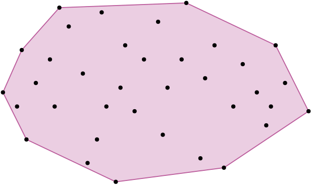
A well-known problem that can be solved classically using the divide-and-conquer paradigm is the convex hull problem; e.g., see Seidel [34]. In the two-dimensional version of this problem, one is given a set, , of points in the plane and asked to output a representation of the smallest convex polygon that contains the points in . (See Figure 1.)
Asymptotically fast classical convex hull algorithms are output sensitive, meaning that their running times depend on both the input size, , and output size, , and there are well-known examples that run in time; e.g., see Kirkpatrick and Seidel [22], Chan [7], and Afshani, Barbay, and Chan [1]. In this paper, we are interested in studying how to efficiently adapt classical output-sensitive divide-and-conquer algorithms, e.g., for convex hull and related problems, to quantum computing models.
Additional Related Work.
There is considerable interest in quantum algorithms for solving computational geometry problems. Sadakane, Sugawara, and Tokuyama [32] give a quantum convex hull algorithm that runs in time,111We use to denote , for some constant . and this time bound is also achieved by Wang and Zhou [36]. Note that if , as can occur, for instance, with points distributed on a circle or parabola, then these algorithms run in time, which is significantly slower than the best classical algorithms. Furthermore, the above quantum algorithms make use of a quantum input data model that assumes that the points are provided in superposition. Many of the procedures require sampling as well, meaning that the algorithms require multiple copies of these input states. We present the algorithm in a standard quantum query model that allows for an even comparison with the existing literature on the subject. In this model, we assume the existence of an oracle that returns the item in the queried index. For completeness, Cortese and Braje [10] showed that there exists a quantum circuit which can take classical data and implement this oracle, with the cost of a logarithmic overhead if the circuit construction time is excluded. Lanzagorta and Uhlmann [24, 23] also describe a quantum convex hull algorithm running in time, which, in their case, is a quantum implementation of the well-known Jarvis march convex hull algorithm using Grover search for the inner loop; see, e.g., [11, 33, 30, 29, 16]. They also describe an algorithm that runs in time, but this result only applies when is small and the points are chosen uniformly at random from a bounded convex region. In addition to this quantum prior work, there is a well-developed body of prior work in classical computing models for computing convex hulls where the points are given pre-sorted in lexicographic order; see, e.g., Ghouse and Goodrich [13], Hayashi, Nakano, and Olarlu [18], Berkman, Schieber, and Vishkin [5], Nakano [27], Goodrich [15], and Nakagawa, Man, Ito, and Nakano [26]. The question we seek to answer in this paper is whether it is possible to leverage this assumption in the quantum setting and obtain asymptotically faster output-sensitive algorithms in the model where the input point set is pre-sorted but with no other assumptions about the distribution of points.
Our Results.
In this paper, we introduce quantum combine and conquer, which is a novel quantum divide-and-conquer paradigm where we perform the combine step before the conquer step and avoid recursion. Our combine-and-conquer paradigm provides a quantum analogue to a classical divide-and-conquer variation that Kirkpatrick and Seidel call “marriage-before-conquest” [20, 21, 22]. We show that using this paradigm it is possible to compute the convex hull of a set of points in the plane in time given that the input is presorted in lexicographic order. As the sorting problem can be reduced to computing the convex hull, and there is no quantum speed-up for sorting [19], we don’t expect quantum algorithms to outperform classical algorithms for this problem in the general case, but this result shows that some reasonable conditions can provide significant speedups. For example, for inputs where is , such as is expected for points uniformly distributed in a convex polygon with a constant number of sides [17], then our method achieves an running time. Similarly, for inputs where is , such as is expected for points uniformly distributed in a disk [17, 31], then our method achieves an running time. In general, our algorithms achieve sublinear running times for sorted input sets for up to almost . Moreover, our results do not depend on any assumptions about the input points coming from a given distribution, such as uniformly distributed points in a convex region. Indeed, our results hold for adversarial chosen point sets, such as points on a circle.
To introduce the combine-and-conquer paradigm, we first apply it to constructing the maxima set of a set of lexicographically sorted points in the plane. Our quantum maxima set algorithm runs in time, where is the size of the output. The key idea to our technique is that there is information that can first be computed globally (the combine step), which partitions the computation into the smaller blocks that then use this information to finish the computation locally and (in a conquer step) without recursion.
We then apply our quantum combine-and-conquer paradigm to the convex hull problem. In this case, the combine step is more complex, in that it includes multiple reductions to two-dimensional linear programming. Nonetheless, we show that the combine steps can still be performed before the conquer steps in this case. As a result, we give a quantum convex hull combine-and-conquer algorithm that runs in time, where is the number of (sorted) input points and is the size of the output. The quantum combine-and-conquer technique provides a novel algorithm design paradigm that may be useful for designing more quantum algorithms that use similar intuition as classical algorithms.
We compare our bounds to previous quantum convex hull algorithms in Table 1. In our algorithm’s input model, the data is encoded by a unitary, such that if the input is a list of points, , then we assume access to a unitary that maps an index to the corresponding element in the array : . The existing literature on quantum solutions to this problem assume that the data is given in a uniform superposition state, . Access to the unitary is a somewhat stronger assumption in that the uniform superposition state can be prepared in unit time given access to . On the other hand, the most natural way to prepare such a state is via access to , as we do.
| Input point set assumptions | Runtime | |
|---|---|---|
| Sadakane, Sugawara, and Tokuyama [32] | Unsorted, arbitrary point set | |
| Wang and Zhou [36] | Unsorted, arbitrary point set | |
| Lanzagorta and Uhlmann [24, 23] | Small , uniformly distributed points | |
| This work | Sorted, arbitrary point set |
2 Preliminaries
We assume basic familiarity with quantum computing; see, e.g., Nielsen and Chuang [28]. A quantum state over qubits is a unit vector of length with complex entries. The computational basis is a basis over quantum states where represents the unit vector of length with a 1 in the -th index and 0 elsewhere. A computational basis state can be used as a classical bit string to simulate any classical algorithm. We can express any quantum state as a weighted sum of these classical basis states,
| (1) |
If at least two in the above are nonzero, we say the state is in superposition. A measurement of the state will collapse the state to with probability . The measurement is destructive in the sense that once it is collapsed, there is no way to go back to without running the circuit to prepare that state. The state where all can be prepared by a circuit of depth 1.
We will assume an input model where the input data is accessible by a unitary that maps an index to the corresponding element in the array . Since quantum operations must be reversible, it is standard to model the action of this unitary by using an index and data register as . We can use linearity to examine the action of this unitary to a state in superposition
| (2) |
from which the data point can be retrieved with probability upon measurement of the index register. Therefore, in this model, we assume that a quantum state representing a distribution of our inputs is preparable in time proportional to the time it takes to prepare the distribution. A transformation from the -bit zero string to a uniform superposition over all -bit strings can be accomplished by a depth 1 circuit where a Hadamard gate is applied to each qubit in parallel.
Much of the existing literature on this subject assumes access to multiple copies of the state in (2). Our assumption of access to is at least as strong of an assumption as having multiple copies of the state. At the same time, it is a standard assumption for states in the form of (2) are generated using access to a unitary like . We therefore compare the performance of our algorithm against the existing literature under equal access to , and we summarize the performance of each in Table 1 under this model.
Quantum Subroutines.
In this section we discuss the two primary quantum subroutines that will be used throughout the paper. The quantum computing components of our algorithms are limited to invocations of these subroutines, and the remainder of the algorithms are done through classical post-processing.
The first subroutine is for preparing superposition states of subsets of points. Our algorithms use the fact that the data is encoded as a sorted list in , and we need to prepare states where is a uniform superposition of consecutive elements in the array starting at index and is a power of 2. Preparation of the begins with a register storing an -bit zero string , and another register large enough to store a point from the dataset, each of which we will call the index and data register respectively. The first step is to set the first bits of the index register to . Next, take the remaining bits in the index register and prepare a uniform superposition state over the bitstrings of length . Finally, apply on this state and the data register to prepare the superposition of states starting from ,
| (3) |
We summarize this process in Algorithm 1. Throughout this paper, we use to represent the subset of storing points in the -th block, and to be the quantum state that encodes this set, as seen in Equation (3).
The second quantum subroutine we use is a quantum max/min finding algorithm due to Durr and Hoyer [12]. This algorithm takes as input a Boolean function, , a comparator, , to maximize (or minimize) over, the index, , of the block to perform the search over, and the total number of blocks, . Our subroutine uses qPrep to prepare the superposition state described in Theorem 1. This has the effect of applying the algorithm only to the points in block , and allows us to search the block in time. Throughout the text, we use the signature, when calling this function, and the output is an element of or null if there are no elements such that . The function can be passed as, say, a classical circuit which can be converted to a quantum circuit.
Theorem 1 (Quantum Maximum/Minimum Finding [12]).
Let be a list of elements represented by bits, and let be the time required to prepare the state,
| (4) |
and the time it takes to query a boolean function . Let be the subset of such that for all . Also, let be some ordering of data values in the data register such that comparisons according to this ordering can be performed in time. Then we can find the maximum (or minimum) value of under the specified ordering in time .
3 Quantum Maxima Sets
In this section, we present a quantum algorithm to solve the maxima set problem using the combine-and-conquer paradigm. In the maxima set problem, we are given a set, , of points in the plane and are tasked with finding the subset of points in that are not dominated by any other points in . We say that a point dominates a point if and . Note that the output size, , can be as small as or as large as .
We assume that the input set is sorted in lexicographic order (first by -coordinates and then by -coodinates in the case of ties), as discussed in the introduction.
Let us begin by reviewing a simple divide-and-conquer algorithm in the classical computing model, which is provided the set, , of points as input in sorted order, and returns the maxima set, (see Preparata and Shamos [30]). The algorithm splits into left and right sets, and , and recursively finds the maxima sets of each. Then it prunes away each point in with smaller -coordinate than the point, , in with maximum -coordinate. The resulting maxima set algorithm, which we give in detail in an appendix, takes time, even when is sorted [30]. Kirkpatrick and Seidel [21] show that if the combine step of finding is performed before the divide and conquer steps, and used to prune points in recursive subproblems, then the running time can be improved to .
For our output-sensitive quantum algorithm, we also perform the combine step before the conquer step, but our goal is to design a quantum algorithm that runs in time without recursion, which requires a more sophisticated approach. We first describe an algorithm where the output size, , is known in advance and later show how to use this algorithm to solve the case where the output size is not known.
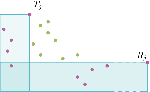
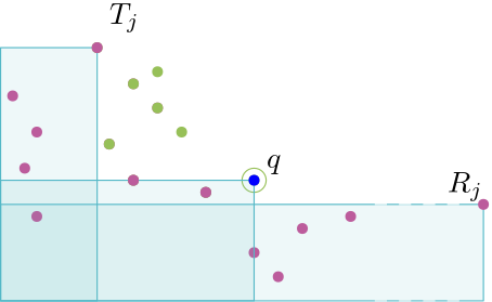
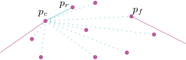
At a high level, the combine-and-conquer approach performs the combine step first before conquering the subproblems. In the maxima set problem, this is achieved in the following way. We begin by dividing our set into different blocks using Algorithm 1. The key observation we use is that we can isolate the problem of finding the maxima set to each of the local blocks once we identify representative information from each block. This representative information is used globally, so we describe the process of finding such information as the combine step. The combine-and-conquer paradigm works for problems where, once the global information is identified, the blocks do not need to communicate with each other for the remainder of the algorithm. In the case of computing the maxima set, the combine step consists of searching for the set of the highest points in each block. Once the set is found, we classically compute the maxima set of . Note that cannot contain more than points, and if a block does not share a point with no points in that block can be in the final output set. Once the points in are identified, we begin the conquer step of the algorithm to find the points in each block that appear in the maxima set. Block number uses information from two points identified in the combine step to restrict the search region. The first is the coordinate of the tallest point within the -th block, which immediately removes all points to the left of it inside block out of the candidate set. The second is the coordinate of the highest point that appears in any of the blocks to the right of block . Note that is left-most point from that is to the right of block . See Figure 2.
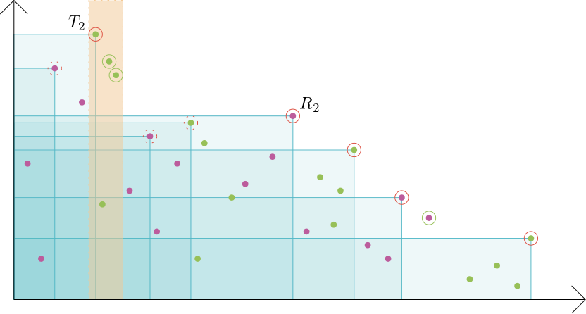
Using and , we can define a Boolean function that takes as input a point and returns 1 if is not dominated by either of and . We then apply Theorem 1 to search for the maximum element in lexicographic order subject to this Boolean function. It turns out that this point is part of the final output set, as tells us it is not dominated by any point in blocks to the right of and tells us it is not dominated by any point in block . We then update to equal this maximal point we found, and repeat this process in block until the Boolean function does not mark any elements in the set. We illustrate the first iteration of this process in Figure 3. Since the output size is , it suffices to run this process times in total across all blocks. Finally, we collect the outputs in the blocks that contain a point in , which takes at most time. See Algorithm 2.
Finally, the case where is unknown can be handled using an approach where we start with a small estimate of , then repeat the procedure using if we discover more than points. Thus, the running time forms a geometric sum that is . See Algorithm 3.
Theorem 2.
There is a quantum algorithm for finding the maxima set of a presorted set of points in the plane in time, where is the size of the output.
Proof.
The Grover searches for the tallest points in each block takes time. Once this set is found, the maxima set of can be computed classically in time. The total time incurred by the calls to CompleteMaximaSet is dominated by the calls to qMax, each of which outputs a point or terminates the call to CompleteMaximaSet. Therefore qMax is called times and each call requires time for a total of time. Note that the condition that the points we are searching over are between and can be done in constant time. The outer loop repeats at most times, whose contribution is suppressed by . Finally, the time to output the points that were found takes time and is dominated by the other parts of the algorithm.
4 Quantum Convex Hulls
In this section, we describe a quantum algorithm to construct the convex hull of points in the plane in time, where is the size of the output. Again, we assume that the input set is sorted in lexicographic order. We follow our combine-and-conquer paradigm, where we use some global properties that can be computed from our subsets to prune off points that do not appear in the output, then use these values to isolate the problem solving within each block. Here, however, the combine step is more complicated that simply finding a point, , with maximum -coordinate.
We begin by reviewing a well-known classical divide-and-conquer algorithm for 2D convex hulls (see, e.g., [11, 33, 30, 29]). The convex hull of a set, , of points in the plane can be described as a union of the polygonal chains that form the upper hull and lower hull of the points, where (resp., ) is the set of edges of with positive (negative) normals. For completeness, we provide a description of a classical divide-and-conquer algorithm for computing in appendix D, which divides into a left set, , and right set, , and recursively finds and . Then it finds the tanget segment bridge between and and prunes away the points under the bridge, resulting in an algorithm running in time. By a well-known point-line duality, which we also review in an appendix, the bridge edge can be found by a solving a two-dimensional linear program; see, e.g., [11, 33, 29].
Lemma 3 (see, e.g., [11, 33, 29]).
Given a vertical line , and a set of points in a plane, one can determine the edge of that intersects (or that no such edge exists) by finding the highest point of intersection between halfplanes.
If we use linear-time 2D linear programming for the bridge-finding step, then the running time for this classical divide-and-conquer algorithm is , even if the points are sorted by -coordinate. Kirkpatrick and Seidel [22] show that this classical running time can be improved to by performing the bridge-finding step before the (recursive) conquer steps. Likewise, our quantum convex hull algorithm also performs this combine step before the conquer steps, but avoids recursion.
Before we give our algorithm, let us review another well-known classical algorithm for computing a two-dimensional convex hull – the Jarvis march algorithm; see, e.g., [11, 33, 30]. In this algorithm, we start with a point, , known to be on the convex hull, such as a point with smallest -coordinate. Then, we find the next point on the convex hull in a clockwise order, by a simple linear-time maximum-finding step. We iterate this search, winding around the convex hull, until we return to the starting point. Since each iteration takes time, this algorithm runs in time. Lanzagorta and Uhlmann [24] describe a quantum assisted version of the Jarvis march algorithm that runs in time, which we review in an appendix.
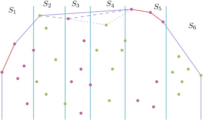
Let be a set of points in the plane sorted lexicographically. For simplicity of expression, let us assume that the points have distinct -coordinates and we are interested in computing the upper hull, , of . As in our maxima set algorithm, let us assume for now that we know the value of , the number of points on the upper hull of to simplify the presentation. We divide into blocks, , of size each by vertical lines, , arranged left-to-right. This is achieved by using Algorithm 1 to partition the input.
At a high level, our quantum combine-and-conquer upper hull algorithm first computes all the bridge edges that are intersected by one of the vertical lines, . This amounts to the combine step of our quantum combine-and-conquer algorithm. Each of these bridge edges belong to the upper hull of ; hence, there are at most such bridges. Importantly, we show how to compute all these bridges in time. Each block of points, , has points, and, of course, there may be remaining upper hull points to compute for each such (between points of tangency for the bridges computed in the combine step). Note that the conquer step for block will return in time if does not contain any endpoints of a bridge edge or if it contains a single point where two bridge edges meet. See Figure 5 showing the edges that come from the combine step and the edges that come from the conquer step.
To compute the remaining convex hull points, then, we perform a modified quantum Jarvis march for each subset, , which runs in time time, where is the number of additional upper hull points found for . Thus, the total time for this second (conquer) phase of our algorithm is
Given this overview, let us next describe how to perform the different steps of our algorithm, beginning with our quantum algorithm for finding all the bridge edges intersecting the vertical lines, , which separate the subsets, , of . At a high level, our combine-step method can be viewed as a quantum adaptation of a classical algorithm by Goodrich [15] for computing the upper hull of a partially sorted set of points.
As mentioned above, by point-line duality, bridge finding is dual to two-dimensional linear programming. In more detail, let be a set of points in the plane, and be a vertical line in this plane. Let be the same set of points after shifting the plane horizontally so that is the -axis. We define a dual plane by taking each point and mapping it to a line . A standard result in computational geometry is that the points in the upper hull of correspond to the lower envelope of the set of lines in the dual plane; see, e.g., [11, 33, 30]. Furthermore, by the duality transformation, the highest point in the lower envelope is the intersection of two lines in the envelope whose slopes transition from positive to negative. Mapping this point to the primal plane gives us the bridge edge we are looking for. Thus, we can reduce the problem of finding a bridge edge to the problem of finding the largest point in the intersection of lower-halfplanes. We also use the following lemma due to Sadakane et al. showing that the problem of computing the highest point in the intersection of halfplanes efficiently using a quantum algorithm.
Lemma 4 (Sadakane et al. [32]).
The highest point in the intersection of lower-halfplanes can be computed in time, using a quantum computer, with probability for any constant given the linear constraints in superposition.
The linear constraints in superposition refers to a state in the following form:
| (5) |
where are the coordinates of each of the points. By point-line duality, the coordinates fully describe the halfplanes in the dual plane.
The output element is a point in the dual plane, which maps back to a line in the primal plane. To determine which points this line intersects, we can run two iterations of minimum finding to find the points in that are on the resulting line by minimizing by the distance to the line. We combine the above two lemmas to a function with the signature,
| (6) |
and it returns the endpoints of the bridge edge as a tuple. This process will also call i,h as needed.
We are now ready to describe the full algorithm. The first step will be to divide our input set into blocks, each containing points. We define a bridge edge to be an edge in the upper hull of whose endpoints are in two different blocks.
To find the bridge edges, we take inspiration from the classical Graham scan algorithm for computing the convex hull. We will be using the fact that if we traverse the convex hull in the clockwise direction, each edge makes a right turn from its previous edge. Since bridge edges are edges in the upper hull, this is true for them as well. We will compute bridge edges between consecutive pairs, but if at any point a left turn is formed between two bridge edges, we know that these edges will not be a part of the upper hull. Critically, this allows us to ignore an entire block of points, and move on to find the bridge edge between the remaining blocks. The details of the above approach are outlined in Algorithm 5.
Lemma 5.
Let be a set of points divided into blocks such that for all and where . Then, the set of bridge edges of this partition can be found in time.
Proof.
Each block’s pending contribution to the bridge edges can only be popped at most once. Thus, the total time it takes for the loop starting at line 3 of Algorithm 5 will be proportional to . For each edge, we must compute the Bridge between sets and , which will take time by lemma 3 and 4. Thus, the total time it takes to find the bridge edges is .
Once the bridge edges are identified, what remains is to find the edges of the convex hull whose end points are in the same block. To do this, we use a quantum assisted Jarvis march. Recall that the Jarvis march is another standard convex hull algorithm in which we start with an edge on the convex hull, then do a search over the remaining points to find the point such that the angle formed between and is maximized.
In each block, , rather than performing a full Jarvis march, however, we start the search from the bridge edge entering from the left, and perform up to Grover searches for the point maximizing the angle until we find the starting point of the bridge edge leaving . We summarize this step in Algorithm 6 and Lemma 6. See also Figure 4.
Lemma 6.
Let be a set of points and , be points on the convex hull of . The part of the convex hull from to in the clockwise direction can be computed in time, where is the number of points on the convex hull from to .
We now combine the above pieces to describe our complete quantum convex hull algorithm. See Figure 5. As was the case in the maxima set algorithm, we begin with a guess for the upper bound of , then during the conquer step detect whether or not we have exceeded this bound. A convex hull requires at least 3 points, so we use 4 as our initial guess, as it is the smallest power of 2 greater than 3. If we exceed our guess, then we double our estimate for and rerun the algorithm. Thus, the running times across all our guesses form a geometric sum that is . See Algorithm 7.
Theorem 7.
There is a quantum algorithm for finding the convex hull of a set of points in lexicographic order that runs in time, where is the size of the output.
Proof.
As observed, the outer loop will run at most times. By lemma 5, FindBridgeEdges takes time. By lemma 6, QuantumJarvisMarch takes time for block , where is the number of points from that lie on the convex hull of the entire points set . Since , the total running time for all the calls to QuantumJarvisMarch is . Finally, printing the discovered points takes time.
In an appendix, we give a lower bound for quantum convex hull that shows our algorithm is optimal up to polylogarithmic factors.
5 Discussion
Afshani, Peyman, and Chan [1] give an instance-optimal classical algorithm for finding 2D convex hulls, which adapts the algorithm by Kirkpatrick and Seidel [22] to run in time, where is a classical-computing structural entropy measure that is never more than . An interesting direction for future work would be to determine if there is a quantum convex hull algorithm that is instance optimal based on a quantum structural entropy measure.
References
- [1] Peyman Afshani, Jérémy Barbay, and Timothy M Chan. Instance-optimal geometric algorithms. Journal of the ACM, 64(1):1–38, 2017. doi:10.1145/3046673.
- [2] Shyan Akmal and Ce Jin. Near-optimal quantum algorithms for string problems. In ACM-SIAM Symposium on Discrete Algorithms (SODA), pages 2791–2832, 2022. doi:10.1137/1.9781611977073.109.
- [3] Jonathan Allcock, Jinge Bao, Aleksandrs Belovs, Troy Lee, and Miklos Santha. On the quantum time complexity of divide and conquer, 2023. doi:10.48550/arXiv.2311.16401.
- [4] Israel F Araujo, Daniel K Park, Francesco Petruccione, and Adenilton J da Silva. A divide-and-conquer algorithm for quantum state preparation. Scientific Reports, 11(1):6329, 2021.
- [5] Omer Berkman, Baruch Schieber, and Uzi Vishkin. A fast parallel algorithm for finding the convex hull of a sorted point set. International Journal of Computational Geometry & Applications, 06(02):231–241, 1996. doi:10.1142/S0218195996000162.
- [6] Ibrahim Cameron, Teague Tomesh, Zain Saleem, and Ilya Safro. Scaling up the quantum divide and conquer algorithm for combinatorial optimization, 2024. arXiv:2405.00861.
- [7] Timothy M. Chan. Optimal output-sensitive convex hull algorithms in two and three dimensions. Discrete & Computational Geometry, 16(4):361–368, 1996. doi:10.1007/BF02712873.
- [8] Daniel Tzu Shiuan Chen, Zain Hamid Saleem, and Michael Alexandrovich Perlin. Quantum circuit cutting for classical shadows. ACM Transactions on Quantum Computing, 5(2):1–21, 2024. doi:10.1145/3665335.
- [9] Andrew M. Childs, Robin Kothari, Matt Kovacs-Deak, Aarthi Sundaram, and Daochen Wang. Quantum divide and conquer, 2022. doi:10.48550/arXiv.2210.06419.
- [10] John A. Cortese and Timothy M. Braje. Loading Classical Data into a Quantum Computer, March 2018. arXiv:1803.01958.
- [11] Mark de Berg, Otfried Cheong, Marc van Kreveld, and Mark Overmars. Computational Geometry: Algorithms and Applications. Springer, 3rd edition, 2008.
- [12] Christoph Durr and Peter Hoyer. A Quantum Algorithm for Finding the Minimum, January 1999. arXiv:quant-ph/9607014.
- [13] Mujtaba R Ghouse and Michael T Goodrich. In-place techniques for parallel convex hull algorithms. In 3rd ACM Symposium on Parallel Algorithms and Architectures (SPAA), pages 192–203, 1991.
- [14] Li-Hua Gong, Wei Ding, Zi Li, Yuan-Zhi Wang, and Nan-Run Zhou. Quantum k-nearest neighbor classification algorithm via a divide-and-conquer strategy. Advanced Quantum Technologies, 7(6):2300221, 2024.
- [15] Michael T. Goodrich. Constructing the convex hull of a partially sorted set of points. Computational Geometry, 2(5):267–278, 1993. doi:10.1016/0925-7721(93)90023-Y.
- [16] Lov K. Grover. A fast quantum mechanical algorithm for database search. In 28th ACM Symposium on Theory of Computing (STOC), pages 212–219, 1996. doi:10.1145/237814.237866.
- [17] Sariel Har-Peled. On the Expected Complexity of Random Convex Hulls. arXiv e-prints, page arXiv:1111.5340, November 2011. doi:10.48550/arXiv.1111.5340.
- [18] T. Hayashi, K. Nakano, and S. Olarlu. An time algorithm to compute the convex hull of sorted points on reconfigurable meshes. IEEE Transactions on Parallel and Distributed Systems, 9(12):1167–1179, 1998. doi:10.1109/71.737694.
- [19] Peter Høyer, Jan Neerbek, and Yaoyun Shi. Quantum Complexities of Ordered Searching, Sorting, and Element Distinctness, pages 346–357. Springer Berlin Heidelberg, 2001. doi:10.1007/3-540-48224-5_29.
- [20] David G. Kirkpatrick and Seidel Raimund. Marriage before conquest: A variation on the divide and conquer paradigm. Technical Report 83-7, University of British Columbia, 1983. URL: https://www.cs.ubc.ca/sites/default/files/tr/1983/TR-83-07.pdf.
- [21] David G. Kirkpatrick and Raimund Seidel. Output-size sensitive algorithms for finding maximal vectors. In 1st Symposium on Computational Geometry (SoCG), pages 89–96, 1985. doi:10.1145/323233.323246.
- [22] David G. Kirkpatrick and Raimund Seidel. The ultimate planar convex hull algorithm? SIAM Journal on Computing, 15(1):287–299, 1986. doi:10.1137/0215021.
- [23] Marco Lanzagorta and Jeffrey Uhlmann. Quantum algorithmic methods for computational geometry. Mathematical Structures in Computer Science, 20(6):1117–1125, 2010. doi:10.1017/S0960129510000411.
- [24] Marco Lanzagorta and Jeffrey K. Uhlmann. Quantum computational geometry. In Quantum Information and Computation II, volume 5436, pages 332–339. SPIE, 2004.
- [25] Junde Li, Mahabubul Alam, and Swaroop Ghosh. Large-scale quantum approximate optimization via divide-and-conquer. IEEE Transactions on Computer-Aided Design of Integrated Circuits and Systems, 42(6):1852–1860, 2023. doi:10.1109/TCAD.2022.3212196.
- [26] Masaya Nakagawa, Duhu Man, Yasuaki Ito, and Koji Nakano. A simple parallel convex hulls algorithm for sorted points and the performance evaluation on the multicore processors. In 2009 International Conference on Parallel and Distributed Computing, Applications and Technologies, pages 506–511, 2009. doi:10.1109/PDCAT.2009.56.
- [27] Koji Nakano. Computation of the convex hull for sorted points on a reconfigurable mesh. Parallel Algorithms and Applications, 8(3-4):243–250, 1996. doi:10.1080/10637199608915555.
- [28] Michael A. Nielsen and Isaac L. Chuang. Quantum Computation and Quantum Information. Cambridge University Press, 10th anniversary edition, 2010.
- [29] Joseph O’Rourke. Computational Geometry in C. Cambridge University Press, 1998.
- [30] Franco P. Preparata and Michael I. Shamos. Computational Geometry: An Introduction. Springer, 2012.
- [31] H. Raynaud. Sur l’enveloppe convexe des nuages de points aleatoires dans . i. Journal of Applied Probability, 7(1):35–48, 1970. doi:10.2307/3212146.
- [32] Kunihiko Sadakane, Norito Sugawara, and Takeshi Tokuyama. Quantum computation in computational geometry. Interdisciplinary Information Sciences, 8(2):129–136, 2002.
- [33] Raimund Seidel. Linear programming and convex hulls made easy. In 6th Symposium on Computational Geometry (SoCG), pages 211–215, 1990. doi:10.1145/98524.98570.
- [34] Raimund Seidel. Convex hull computations. In Handbook of Discrete and Computational Geometry, pages 687–703. Chapman and Hall/CRC, 2017.
- [35] Teague Tomesh, Zain H. Saleem, Michael A. Perlin, Pranav Gokhale, Martin Suchara, and Margaret Martonosi. Divide and conquer for combinatorial optimization and distributed quantum computation. In 2023 IEEE International Conference on Quantum Computing and Engineering (QCE), volume 01, pages 1–12, 2023. doi:10.1109/QCE57702.2023.00009.
- [36] Cheng Wang and Ri-Gui Zhou. A quantum search algorithm of two-dimensional convex hull. Communications in Theoretical Physics, 73(11):115102, September 2021. doi:10.1088/1572-9494/ac1da0.
- [37] Qisheng Wang. A note on quantum divide and conquer for minimal string rotation, 2022. doi:10.48550/arXiv.2210.09149.