A Sparse Multicover Bifiltration of Linear Size

Abstract
The -cover of a point cloud of at radius is the set of all those points within distance of at least points of . By varying and we obtain a two-parameter filtration known as the multicover bifiltration. This bifiltration has received attention recently due to being choice-free and robust to outliers. However, it is hard to compute: the smallest known equivalent simplicial bifiltration has simplices. In this paper we introduce a -approximation of the multicover bifiltration of linear size , for fixed and . The methods also apply to the subdivision Rips bifiltration on metric spaces of bounded doubling dimension yielding analogous results.
Keywords and phrases:
Multicover, Approximation, Sparsification, Multiparameter persistenceCopyright and License:
2012 ACM Subject Classification:
Mathematics of computing Topology ; Theory of computation Computational geometryAcknowledgements:
The author would like to thank his advisor Michael Kerber for helpful comments. He would also like to deeply thank an anonymous reviewer for many comments that helped to substantially improve the exposition. Part of the writing was carried out while the author was visiting Yasuaki Hiraoka’s group at the Kyoto University Institute of Advanced Study.Funding:
This research was funded in whole, or in part, by the Austrian Science Fund (FWF) 10.55776/P33765.Editors:
Oswin Aichholzer and Haitao WangSeries and Publisher:
1 Introduction
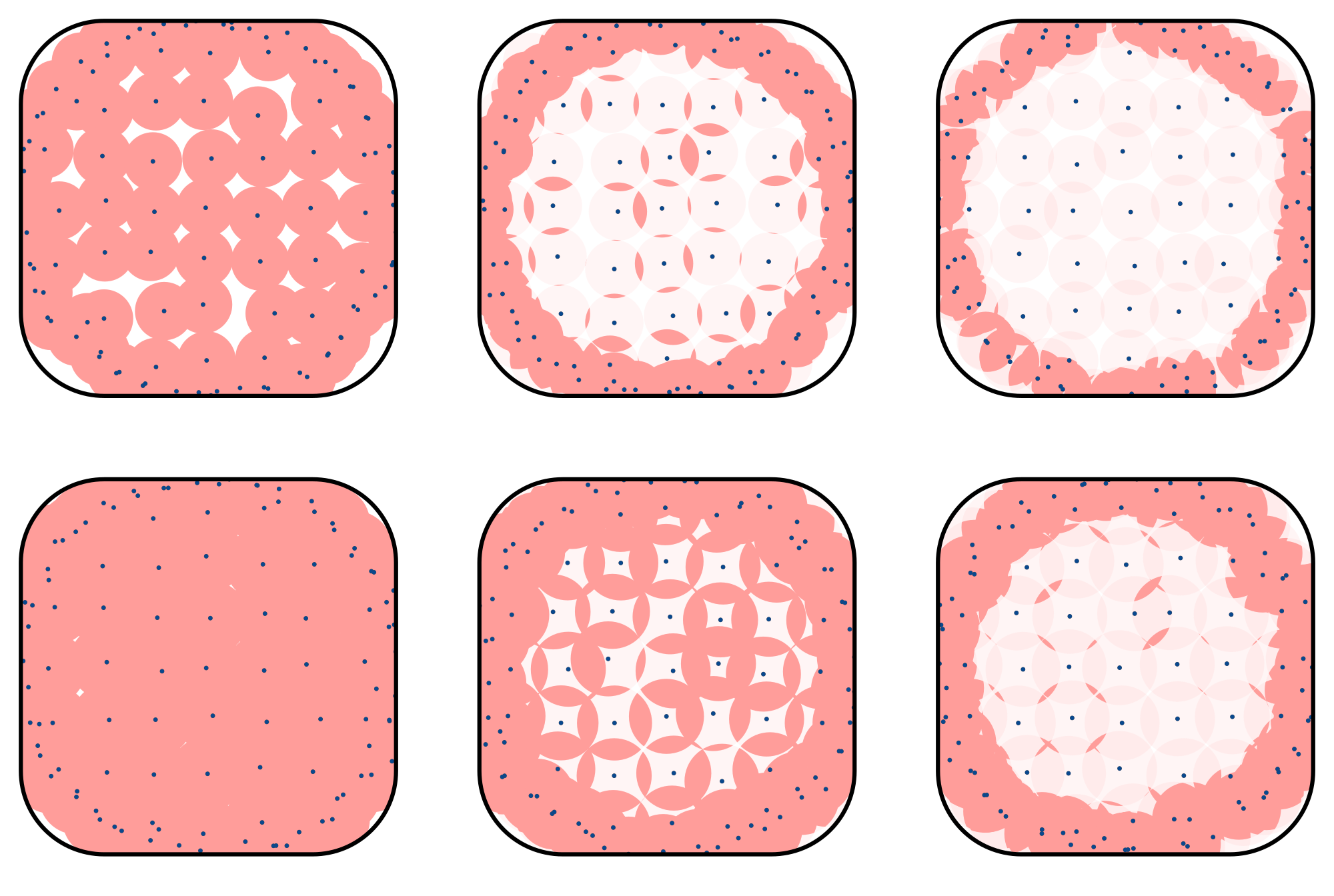
This paper aims to approximate the multicover bifiltration of a finite subset of , depicted in Figure 1. The -cover for a scale is given by all those points covered by at least balls of radius around the points of :
For any and , we have that and as such the assemble into a bifiltration known as the multicover bifiltration.
The multicover bifiltration offers a view into the topology of the point cloud across multiple scales, in a way that is robust to outliers [7]. However, computing the multicover bifiltration remains a challenge. Current exact combinatorial (simplicial or polyhedral) methods [34, 28] are expensive, of size , and previous approximate methods [12, 9] are in general exponential and only linear on when taking to be at most a constant.
For general metric spaces, instead of subsets of , an analogue of the multicover is the subdivision Rips bifiltration [53]. As the multicover, it has received attention recently, both in its theoretical [7] and computational aspects [42, 43, 41], where it faces similar challenges as the multicover. Previous approximation schemes [44, 7, 42, 43, 41] are of size polynomial (but not linear) in , see the related work section below.
In this paper, we define a simplicial bifiltration, the sparse subdivision bifiltration (Definition 13), that -approximates the multicover and that is of linear size , independently of and for fixed and . It can be computed in time , where is the spread of , the ratio between the longest and shortest distances between points in . In addition, the methods extend to obtain analogous results for the subdivision Rips bifiltration for metric spaces of bounded doubling dimension, as we discuss in Section 6.
The sparse subdivision bifiltration is (homotopically) equivalent to the sparse multicover bifiltration (Definition 6), a bifiltration of subsets of . It is via that the sparse subdivision bifiltration -approximates the multicover, by which we mean that
for any and , as shown in Theorem 8. In other words, the sparse subdivision bifiltration and the multicover are (multiplicatively) -homotopy-interleaved [6].
This approximation is analogous to the one obtained by Cavanna, Jahanseir and Sheehy [16] for the case of fixed , and our techniques can be traced back to their work; see the related work section. A key principle is that instead of balls of radius , the sparse multicover bifiltration is based on sparse balls (Definition 1), understood as balls with a lifetime of three phases: on the first phase they grow normally (at scale they have radius ), and then they are slowed down (they keep growing but at scale they have radius less than ), before eventually disappearing. Cavanna, Jahanseir and Sheehy [16] (there is a video [15]) do the same, with technical differences that include stopping balls from growing, rather than growing slow. The size bounds here are also an adaptation of their methods, as well as the technique of lifting the construction one dimension higher, as in the cones of Section 3.1.
We guarantee that when a sparse ball disappears it is approximately covered by another present sparse ball, and we keep track of which present sparse ball covers which disappeared sparse ball via a covering map (Definition 4). A sparse ball is weighted by as many sparse balls it approximately covers according to the covering map – the sparse -cover consists of those points covered by sparse balls whose total weight is at least .
1.1 Motivation and related work
For , the -cover is the union of balls of radius around points of . The union of balls is commonly used in reconstructing submanifolds from samples [46, 4, 3] and is a cornerstone of persistent homology methods in topological data analysis, being homotopy equivalent to the Čech complex and the alpha complex [31, 32], and related to the (Vietoris-)Rips complex. The union of balls assembles into a -parameter filtration: by increasing the scale parameter we obtain inclusions , for . Taking the homology of each , we obtain a persistence module, an algebraic descriptor of the topology of the filtration across the different scales. Such a persistence module is stable to perturbations of the points [26, 25], but is not robust to outliers (already appreciated in the first column of Figure 1) and insensitive to differences in density in the point cloud.
There are multiple methods that address the lack of robustness to outliers and changes in density within the -parameter framework. These include density estimation [47, 20, 8], distance to a measure [18, 38, 39, 19, 2, 1, 11, 10], and subsampling [5]. However, they all depend on choosing a parameter. The problem is that it is not clear how to choose such a parameter for all cases, and such a choice might focus on a specific range of scales or densities. We refer to [7, Section 1.7] for a complete overview of the methods and their limitations.
It is then natural to consider constructions over two parameters, scale and density. Examples include the density bifiltration [13], degree bifiltration [44], and the multicover, closely related to both the distance to a measure [18] and -nearest neighbors [53]. The advantage of the multicover is that it does not depend on any further choices (like choosing a density estimation function) and that it is robust to outliers, as a consequence of its strong stability properties [7].
However, one currently problematic aspect of the multicover is its computation. Sheehy [53] introduced an influential simplicial model of the multicover called the subdivision Čech bifiltration, based on the barycentric subdivision of the Čech filtration. It has exponentially many vertices on the number of input points, making its computation infeasible. A crucial ingredient in the theory is the multicover nerve theorem [53, 14, 7] that establishes the topological equivalence (see Section 3.1 for a precise definition) of the subdivision Čech and multicover bifiltrations. Such a multicover nerve theorem has its analogue for the sparse multicover, the sparse multicover nerve theorem (Theorem 14).
Dually to an hyperplane arrangement in , Edelsbrunner and Osang [34, 33] define the rhomboid tiling and use it to compute, up to homotopy, slices (fixing and varying or viceversa) of the multicover bifiltration. Corbet, Kerber, Lesnick and Osang [28, 27] build on it to define two bifiltrations topologically equivalent to the multicover, of size .
Recently, Buchet, Dornelas and Kerber [12] introduced an elegant -approximation of the multicover whose -skeleton has size that is linear on but that incurs an exponential dependency on the maximum order we want to compute. A crucial difference between our work and the Buchet-Dornelas-Kerber (BDK) sparsification is that BDK work at the level of intersection of balls, while we work directly at the level of balls. This starting point is what allows us to ultimately obtain a construction of linear size, independently of .
In addition, BDK work by freezing the lenses: at a certain scale they stop growing. It is not clear (or is technically challenging, in the words of BDK) how to compute exactly the first scale at which freezing lenses first intersect – a problem they sidestep by discretizing the scale parameter (at no complexity cost). In contrast, by letting sparse balls grow slowly at a certain rate, rather than freezing them completely, we can compute their first intersection time exactly, as we explain in Section 5.3.
Sparsification.
Our methods are part of a line that can be traced to the seminal work of Sheehy [54, 52] to obtain a linear size approximation of the Vietoris-Rips filtration. Subsequently, Cavanna, Jahanseir and Sheehy [16] simplified and generalized Sheehy’s methods to obtain a linear size -approximation of the union-of-balls filtration . They construct a filtration such that , resembling Theorem 8 here. Moreover, the sparse balls we use here are directly inspired by their methods: they use balls that grow normally, stop growing, and eventually disappear.
These methods, broadly referred to as sparsification, have also been applied to the Delaunay triangulation [55] and, as already mentioned, the multicover itself [12]. A fundamental ingredient in many of these constructions is the greedy permutation [49, 37, 30], or variants of it, that we also use in the form of persistent nets (Section 2.1).
General metric spaces.
In general metric spaces, an analogue of the subdivision Čech bifiltration of Sheehy is the subdivision Rips bifiltration. Its computation faces similar challenges, and, in fact, no subexponential size simplicial model of it exists [42]. Thus, there has been recent interest in approximations of subdivision Rips. Indeed, the degree Rips bifiltration [44], which can be shown to be a -approximation [7] whose -skeleton has size , and has been implemented [44, 48, 50]. Furthermore, it was recently shown that subdivision Rips admits -approximations whose -skeleta have the same size as degree Rips [41, 42]. Most recently, Lesnick and McCabe [42, 43], in the more particular case of metric spaces of bounded doubling dimension (which include Euclidean spaces), give a -approximation of subdivision Rips whose -skeleton has simplices, for fixed and dimension. Our methods also apply to the subdivision Rips setting, yielding analogous results, as discussed in Section 6.
Miniball.
In Section 5.3, we compute the first scale at which a set of sparse balls have non-empty intersection, for Euclidean space. If instead of sparse balls we would be using usual balls, such a scale would be the radius of the minimum enclosing ball of the centers of the balls – the miniball problem, first stated by Sylvester in 1857 [56]. Our solution to the analogous problem for sparse balls has its origin in Welzl algorithm [57], which takes randomized linear time on the number of centers. The miniball problem is of LP-type as introduced later by Matoušek, Sharir and Welzl [45], and Welzl algorithm for the miniball can be generalized to the Matoušek-Sharir-Welzl (MSW) algorithm for LP-type problems. Fischer and Gärtner [35] solve the problem of computing the minimum enclosing ball of balls – generalizing the miniball – via the MSW-algorithm in a way that is practical and efficient, as in the implementation in the CGAL library [36]. Here, we frame the problem of computing the first scale of intersection of sparse balls as an LP-type algorithm and show how to solve it as an extension of Fischer and Gärtner’s methods. The miniball and similar problems have also been stated and solved through the geometric optimization point of view, see [29, 17] and references therein.
2 A sparse multicover bifiltration
In this section we introduce the sparse multicover bifiltration. As already noted in the introduction, instead of using balls of radius , the sparse multicover involves balls with a lifetime of three phases: they start as usual balls of radius at scale , at some point they start to grow slowly, that is, they have radii smaller than at scale , and eventually they disappear. We call this version of balls sparse balls. For their definition and the subsequent proofs we use the notion of persistent nets, which we define first.
2.1 Persistent nets
Persistent nets, defined below, are a reinterpretation of farthest point sampling, or greedy permutations, as known in the sparsification literature [16, 55, 12], and as such are guaranteed to exist by Gonzalez algorithm [37]. We will revisit these concepts in Section 5.
Let be a finite metric space. We say that a subset is a -net for a radius , if it is
-
1.
a -covering: for every there is an with , and
-
2.
a -packing: for every two we have .
In the spirit of persistence, a persistent net of is a collection of -nets , one for each , such that for any two we have .
The insertion radius of a point , with respect to a persistent net , is the supremum of those such that . There is a large enough so that is a single point (it has to be a -packing), and so there is only one point with .
2.2 Sparse balls
In what follows, we work over a fixed finite subset , with equipped with any norm. We also fix an error parameter and a persistent net of , that we often drop from the notation. We define the slowing time of a point by
Definition 1.
We define the sparse ball of at scale as:
where denotes the closed ball around of radius , and is a radius function: any strictly increasing function such that
-
on the interval , is , and
-
on the interval , satisfies
For example, the radius function of a point can be
but other options are useful for computation (Section 5.3). In any case, the sparse ball of has radius up to scale , it then starts to grow slowly with radius at most , until eventually disappearing at scale . We say that the sparse ball around is slowed at scale if .
The functions and are defined in this way for technical reasons related to properties of the sparse multicover that we will prove shortly. For now, let us say that whenever a sparse ball disappears (that is, at scale ), it is covered by another non-slowed sparse ball:
Lemma 2.
Let be a point and write . There exists a point such that and .
Proof.
Note that the sparse ball of has radius at most . At scale , the centers of the non-slowed balls are precisely the -net . Thus, since , there is a in such that the sparse ball around covers the ball around of radius ,
2.3 Covering map
One of the intuitive principles behind the sparse multicover is that, at every scale , the non-empty sparse balls approximately cover the balls of radius around all the points of . Below, we formally define a map that takes each point to the non-empty sparse ball that approximately covers the ball of .
Definition 3.
We define the covering sequence of a point as follows: we set and, recursively, given and if , we set to be the nearest neighbor (breaking ties arbitrarily) of among those points with . In other words, the nearest neighbor among those points whose sparse balls are non-slowed when the sparse ball of disappears.
Definition 4.
For each scale , the covering map takes to the first in its covering sequence whose sparse ball is non-empty at scale .
For a point and , we say that , the cardinality of its preimage under the covering map, is its covering weight.
We will use the following lemma multiple times. It describes how the covering map inherits covering and packing properties from the persistent net.
Lemma 5.
The covering map has the following properties, for each :
-
1.
The image is the set of points whose sparse balls at radius are non-empty,
-
2.
the points in are -packed, and
-
3.
for each and writing , .
Proof.
The first property is by definition.
For the second, by the previous property the sparse ball of a has not disappeared at scale , and thus . This gives that , which implies what we want by the definition of and persistent net.
For the third, if there is nothing to prove. Otherwise, let be the point directly before in the covering sequence of , and write . By construction, and . Thus, is in , and is the nearest neighbor of in such subset. We conclude that .
2.4 The sparse multicover
We can write the -cover for a scale as
In parallel, the sparse multicover uses sparse balls instead of balls, and the covering weight instead of the number of balls:
Definition 6.
The sparse -cover , for and , is the set of points covered by sparse balls at scale whose sum of covering weights at scale is at least ,
The sparse multicover is the bifiltration given by the sparse covers:
Proposition 7.
For and , we have .
Proof.
Let and let be a subset whose sparse balls of radius cover with covering weight at least . Take and note that there are at least points in . For each , we claim that the sparse ball of (the point that “covers” at scale ) also contains . Proving the claim finishes the proof, as the sum of covering weights of is at least .
We write and . The claim is immediate if . Otherwise, note that necessarily , because the point with infinite insertion radius is unique. Also note that and, thus, . This fact, together with the triangle inequality and Lemma 5, gives
The sparse multicover approximates the multicover:
Theorem 8.
Writing , we have
Proof.
We start with the first inclusion. Let , which implies that there is a subset of points such that for all .
Let and note that the sum of covering weights is at least . It is left to show that every sparse ball around points of at scale contains . Consider a point and write . Note that necessarily , because otherwise the sparse ball of has disappeared by scale . We have
Now we do a case distinction. If , we have
and otherwise , so we have
We now prove the second inclusion. Let . This means that there exists a subset whose sparse balls cover at radius with covering weight at least . Consider . Then, by definition, and it is left to show that for each we have . Indeed, writing ,
We do a case distinction again. If , then
Otherwise, if ,
3 An equivalent simplicial bifiltration
We look for a bifiltration of simplicial complexes that is homotopically equivalent, as defined shortly, to the sparse multicover bifiltration. This will be the sparse subdivision bifiltration, which is an extension of the subdivision Čech bifiltration of Sheehy [53].
3.1 Homotopically equivalent bifiltrations
We now recall the fundamental definitions of the homotopy theory of filtrations, where filtrations are viewed as diagrams, as is standard; see, e.g., [7]. Let be a bifiltration of topological spaces indexed, in our case, by radii and order ; that is, a collection of topological spaces , one for each and , together with a continuous map for every and , such that is the identity and the following diagram commutes
A pointwise weak equivalence between two bifiltrations and , is a collection of weak homotopy equivalences such that the following diagram commutes for every and :
Pointwise weak equivalence is not a equivalence relation, but the following is. Two bifiltrations and are weakly equivalent if there exists a zigzag of pointwise homotopy equivalences that connect them:
3.2 The sparse subdivision bifiltration
We now define the sparse subdivision bifiltration and prove that is weakly equivalent to the multicover bifiltration. As already mentioned, the sparse subdivision bifiltration is an extension of Sheehy’s subdivision Čech bifiltration [53], which we review first.
Subdivision Čech bifiltration.
We start with the following extension of the Čech complex:
Definition 9.
For a given scale and order , the -Čech poset is
with the order given by inclusion.
The -Čech poset is (the face poset of) the usual Čech simplicial complex. The collection of the Čech posets assemble into a bifiltration that we call the multi-Čech bifiltration : for any and , we have .
To obtain a bifiltration of simplicial complexes we take the order complex pointwise, as below. By order complex of a poset we mean the simplicial complex whose set of vertices is and whose -simplices are the chains of of length .
Definition 10.
The subdivision Čech bifiltration is given by with the internal maps being the inclusions.
The subdivision Čech bifiltration is usually defined directly at the level of the subdivision of the Čech complex [53], rather than through the multi-Čech bifiltration. Now we can state the multicover nerve theorem [53, 14, 7]:
Theorem 11 (Multicover nerve theorem).
The multicover bifiltration is weakly equivalent to the subdivision Čech bifiltration .
Sparsification.
We now extend the subdivision Čech bifiltration and the multicover nerve theorem to the sparse multicover bifiltration. As in the definition of the sparse multicover, we replace the balls with sparse balls and the cardinality with the covering weight, resulting in the following definition; to be compared with the definition of -Čech poset (Definition 9.)
Definition 12.
For a given scale and order , we define the sparse Čech poset to be
with the order given by inclusion.
In the definition, the union is there to guarantee that the assemble into a bifiltration, because now sparse balls disappear, unlike before; this is the combinatorial analogue of taking cones as in Cavanna, Jahanseir and Sheehy’s work [16]. Again taking the order complex:
Definition 13.
The sparse subdivision bifiltration is given by taking , the order complex of the sparse intersection poset .
In other words, the -simplices of are sequences of subsets of points, all in and where each containment is strict.
Theorem 14 (Sparse multicover nerve theorem).
The sparse subdivision bifiltration is weakly equivalent to the sparse multicover .
The proof is in the full version. It reduces to the multicover nerve theorem, incorporating the covering weight and using the cones strategy of Cavanna, Jahanseir and Sheehy [16].
4 Size
We are now ready to bound the size of the sparse subdivision bifiltration. Specifically, we bound the number of simplices in the largest complex in the bifiltration, and show that each simplex is born at a constant number of critical grades. We say that the grade is critical for a simplex , if for all and , but for any and .
4.1 Number of simplices
The rest of this section is dedicated to proving the following theorem. We write to refer both to the bifiltration and to the largest complex in the bifiltration, , when no confusion is possible.
Theorem 15.
The bifiltration has simplices for fixed and dimension .
The following argument is analogous to the one used in previous sparse filtrations [54, 16]. Consider the map that takes each simplex to the minimum point in with respect to the order given by their insertion radius , breaking ties arbitrarily. The points in each preimage of this map are not too far from each other:
Lemma 16.
Let be a simplex and let . The points are contained in a ball of radius around .
Proof.
Since the sparse ball around is empty at scales greater than , any intersection between the sparse balls of must happen at a scale . Let be any point in this intersection. It follows that for any other we have .
Lemma 17.
For each , the number of simplices mapped to under is , for fixed and dimension .
Proof.
Let be the set of all points in simplices such that . It suffices to show that has points, for fixed and . Let . We claim that . Indeed, for every we have , by the definition of , and thus the sparse ball of is non-empty at scale .
By Lemma 16, the points in are contained in a ball of radius , and, by Lemma 5, they are -packed, because as shown. By comparing the volume of balls of radius and , we conclude that consists of points.
All in all, there can be at most simplices, since at most a constant number, for a fixed and , of simplices is mapped to each point, finishing the proof of the theorem.
4.2 Critical grades
The sparse subdivision bifiltration, unlike the subdivision Čech bifiltration, is multicritical, which means that each simplex may have multiple critical grades. Let us briefly describe the critical grades of a simplex . Ordering the critical grades by scale , the first critical grade has scale equal to the first scale at which the sparse balls around the points intersect, and order equal to the sum of the covering weights of the points of at such an scale. Further critical grades of correspond to scales at which the covering weight of the points of increase, until one of the associated sparse balls disappears. Still, there are not many critical grades, as another packing argument shows:
Theorem 18.
Each simplex in has critical grades, for fixed and .
Proof.
Let and let . The simplex has no critical grade with scale greater than , because the sparse ball of disappears then. Thus, we bound the number of scales at which the sum of covering weights of the points of increases, which bounds the number of critical grades of .
By the proof of the Lemma 17, the points in are a -packing, where . Thus, any intersection between balls around points in must happen at scales at least , and thus we are interested in the range of scales .
Let be the subset of points whose sparse ball disappears in the interval , meaning and, as a result, the covering weight of a point in increases, meaning there is a point such that and a point are one after the other in the covering sequence of , that is, and . To finish the argument, it suffices to show that . First, note that . It follows that the points in are -packed, by Lemma 5.
5 Computation
We show how to compute the sparse subdivision bifiltration. The first step is computing a persistent net and the covering map. As already mentioned in Section 2.1 this reduces to computing a greedy permutation. The next step is to compute all potential simplices that appear in the bifiltration, as those consisting of points around balls like those of Lemma 16; for which we use a suitable proximity data structure. Finally, to obtain the critical grades of the simplices we can use the covering map and the minimum scale at which a subset of the sparse balls intersect. The problem of computing this minimum scale, in the Euclidean case, can be written as a LP-type problem [45], and we show how to solve it, much like computing the smallest enclosing ball of balls [35]. All these steps can be done in time, where is the spread of , the ratio between the longest and shortest distances in .
5.1 Greedy permutations
Let be an ordering of the points in . Such a sequence is called greedy if for every and prefix , one has
where . The distance is the insertion radius of , where we take by convention. A greedy permutation gives a persistent net by taking .
Gonzalez [37] gives a method to compute a greedy permutation. It consists of phases, divided in an initialization phase and update phases. At the end of phase , it maintains a subset and for each its Voronoi set: the subset of points in that are closer to than to any other point in . We break ties arbitrarily but consistently (say, by minimum index in ), so that the Voronoi sets form a partition of . In the initialization phase we pick a random point and we set its Voronoi set to be every other point. In the update phase , we obtain the new set of leaders by adding to the point whose distance to is maximal, and updating the Voronoi sets. This algorithm can be implemented in -time by going over the whole set of points during each phase. An algorithm of Clarkson [23, 24], which also maintains the Voronoi sets, can be shown to take -time [40], and has been implemented [24, 51].
As mentioned, at every phase of the algorithm, each point is assigned a Voronoi set of a point : its nearest neighbor among those in . We call the sequence of such points , as the algorithm progresses, the sequence of leaders of a point . Such a sequence necessarily starts with and ends with the point itself.
From the sequence of leaders we can obtain the covering map. The covering sequence of a point is a subsequence of its sequence of leaders, in reverse order. To see this, note that the covering sequence of starts with itself, as in the reversed sequence of leaders. Then, when the sparse ball of disappears the next point in its covering sequence is its nearest neighbor among those points with non-slowed sparse ball. This set of points with non-slowed sparse ball is necessarily equal to one of the subsets we have encountered through the execution of the algorithm. In addition, balls are slowed in the same order as the reversed sequence of leaders. All in all, we conclude the following:
Lemma 19.
A persistent net, the insertion radius of all the points, and the covering map can be computed in time .
5.2 Neighborhoods
We also need to find those subsets of points whose sparse balls have a non-empty intersection, at any scale. By Lemma 16, any such subset is contained in a ball of radius around , where is the point of minimal insertion point in . Making use of this observation, and following [12], given a point , we call the points of higher insertion radius than the one of and within distance its friends. Note that the number of friends of a point is , because we are only considering points of higher insertion radius, as in Lemma 17. Once we have computed the friends of , we can go over every possible subset and check whether the associated sparse balls intersect at some scale, which is done in the following section. This procedure is similar to other sparsification schemes [16, 12].
To compute the friends of every point, we can use a proximity search data structure as follows. First, we initialize it empty. In decreasing order of insertion radius (that is, the order given by the greedy permutation), we add the points one by one. After adding a point , we query all the points within distance from .
Cavanna, Jahanseir and Sheehy [16] gives such a data structure to compute all friends in such a way in time , again for fixed and . In practice one can also use the related greedy trees [22], which have been implemented [51].
Lemma 20.
Computing the friends of all points can be done in time.
5.3 Intersection of sparse balls
We now show how to compute the scale at which a subset of sparse balls first intersect, if they do so. We do it only for the Euclidean case; the -norm, which is also of interest, is an easier case, since it is enough to compute the intersection times pairwise. We show that this problem is of LP-type [45] and can be solved efficiently following the blueprint of the LP-algorithm for computing the smallest enclosing ball of balls [35], which is efficient in practice and implemented in CGAL [36].
A specific radius function.
Let us choose a specific radius function first, with the added restriction that . For a point , we take
| (1) |
where, . See Figure 3. It can be checked that is indeed a radius function.
Solving a problem.
Equipped with the radius function above and given a subset of points , we consider the problem
| (2) | |||||
| subject to | |||||
Now it is apparent why we chose the specific radius function of Equation 1: the right side of the inequalities above is linear on . We claim that the solution of this problem gives the minimum scale at which the sparse balls of have non-empty intersection, if such a scale exists. Let and be the solution of the problem above (a unique solution always exists, see the full version). One can check that is the minimum scale at which the balls around points first intersect, by noting that whenever . Thus, is the minimum scale at which the sparse balls of intersect, unless a sparse ball disappears before then, that is, unless for any .
We solve the problem of Equation 2 via a more general problem. Given a set of constraints, each being a triple consisting of a point , a positive real constant and a non-negative real constant , we look for
| (M) | ||||
| subject to |
The problem of Equation 2 is an instance of (M) with constraints.
Note that by taking a set of points and setting and , the solution to (M) above is the smallest enclosing ball of the points (with radius ). As already hinted, the smallest enclosing ball can be computed as a LP-type problem [45]. In the full version, we show how to solve (M) as a LP-type problem following the strategy of the smallest enclosing ball of balls [35, 58].
6 Discussion
We have introduced a -approximation of the multicover that is of linear size, which is optimal, for fixed dimension and error . As it is usual in sparsification and similar approximations, such a bound on the size (and computation) hides constants that have an exponential dependency on . The computation time is dominated by the computation of the greedy permutation, which is , where is the spread. We remark that one can compute a -approximate greedy permutation in time [40, 21].
Although so far we have focused on the multicover (and subdivision) bifiltration in , the sparsification scheme works in general metric spaces, where one takes the subdivision Rips bifiltration. Indeed, and as expanded upon in the full version, the construction presented here, for the same reasons as the construction of Cavanna, Jahanseir and Sheehy [16] that inspired it, does not depend on the chosen norm, and the size bounds can be seen to extend to spaces with bounded doubling dimension. Thus, we can isometrically embed any finite metric space into , where the Rips complex is equal to the Čech complex, and take the sparse multicover there.
References
- [1] Hirokazu Anai, Frédéric Chazal, Marc Glisse, Yuichi Ike, Hiroya Inakoshi, Raphaël Tinarrage, and Yuhei Umeda. DTM-Based Filtrations. In Gill Barequet and Yusu Wang, editors, 35th International Symposium on Computational Geometry, SoCG 2019, volume 129 of LIPIcs, pages 58:1–58:15, 2019. doi:10.4230/LIPIcs.SoCG.2019.58.
- [2] Hirokazu Anai, Frédéric Chazal, Marc Glisse, Yuichi Ike, Hiroya Inakoshi, Raphaël Tinarrage, and Yuhei Umeda. DTM-Based Filtrations. In Nils A. Baas, Gunnar E. Carlsson, Gereon Quick, Markus Szymik, and Marius Thaule, editors, Topological Data Analysis, pages 33–66. Springer, 2020. doi:10.1007/978-3-030-43408-3_2.
- [3] Dominique Attali, André Lieutier, and David Salinas. Vietoris-Rips complexes also provide topologically correct reconstructions of sampled shapes. In Proceedings of the Twenty-Seventh Annual Symposium on Computational Geometry, SoCG 2011, pages 491–500, June 2011. doi:10.1145/1998196.1998276.
- [4] Dominique Attali, André Lieutier, and David Salinas. Vietoris–Rips complexes also provide topologically correct reconstructions of sampled shapes. Computational Geometry, 46(4):448–465, May 2013. doi:10.1016/j.comgeo.2012.02.009.
- [5] Andrew J. Blumberg, Itamar Gal, Michael A. Mandell, and Matthew Pancia. Robust Statistics, Hypothesis Testing, and Confidence Intervals for Persistent Homology on Metric Measure Spaces. Foundations of Computational Mathematics, 14:745–789, August 2014. doi:10.1007/s10208-014-9201-4.
- [6] Andrew J. Blumberg and Michael Lesnick. Universality of the homotopy interleaving distance. Transactions of the American Mathematical Society, 376:8269–8307, 2023. doi:10.1090/tran/8738.
- [7] Andrew J. Blumberg and Michael Lesnick. Stability of 2-Parameter Persistent Homology. Foundations of Computational Mathematics, 24:385–427, 2024. doi:10.1007/s10208-022-09576-6.
- [8] Omer Bobrowski, Sayan Mukherjee, and Jonathan E. Taylor. Topological consistency via kernel estimation. Bernoulli, 23(1):288–328, February 2017. doi:10.3150/15-BEJ744.
- [9] Mickaël Buchet, Bianca B. Dornelas, and Michael Kerber. Sparse Higher Order Čech Filtrations. In Erin W. Chambers and Joachim Gudmundsson, editors, 39th International Symposium on Computational Geometry, SoCG 2023, volume 258 of LIPIcs, pages 20:1–20:17, 2023. doi:10.4230/LIPIcs.SoCG.2023.20.
- [10] Mickaël Buchet, Frédéric Chazal, Steve Y. Oudot, and Donald R. Sheehy. Efficient and robust persistent homology for measures. In Proceedings of the Twenty-Sixth Annual ACM-SIAM Symposium on Discrete Algorithms, SODA 2015, pages 168–180, January 2015. doi:10.1137/1.9781611973730.13.
- [11] Mickaël Buchet, Frédéric Chazal, Steve Y. Oudot, and Donald R. Sheehy. Efficient and robust persistent homology for measures. Computational Geometry, 58:70–96, October 2016. doi:10.1016/j.comgeo.2016.07.001.
- [12] Mickaël Buchet, Bianca B. Dornelas, and Michael Kerber. Sparse Higher Order Čech Filtrations. Journal of the ACM, 71(4):1–23, August 2024. doi:10.1145/3666085.
- [13] Gunnar Carlsson and Afra Zomorodian. The Theory of Multidimensional Persistence. Discrete & Computational Geometry, 42(1):71–93, July 2009. doi:10.1007/s00454-009-9176-0.
- [14] Nicholas J. Cavanna, Kirk P. Gardner, and Donald R. Sheehy. When and Why the Topological Coverage Criterion Works. In Proceedings of the Twenty-Eighth Annual ACM-SIAM Symposium on Discrete Algorithms, SODA 2017, pages 2679–2690, January 2017. doi:10.1137/1.9781611974782.177.
- [15] Nicholas J. Cavanna, Mahmoodreza Jahanseir, and Donald R. Sheehy. Visualizing Sparse Filtrations. In Lars Arge and János Pach, editors, 31st International Symposium on Computational Geometry, SoCG 2015, volume 34, pages 23–25. Schloss Dagstuhl – Leibniz-Zentrum für Informatik, 2015. doi:10.4230/LIPICS.SOCG.2015.23.
- [16] Nicholas J. Cavanna, Mahmoodreza Jahanseir, and Donald R. Sheehy. A Geometric Perspective on Sparse Filtrations. In Proceedings of the 27th Canadian Conference on Computational Geometry, pages 116–121, 2015. arXiv:1506.03797.
- [17] Mark E. Cawood and P. M. Dearing. The weighted Euclidean one-center problem in . Computational Optimization and Applications, August 2024. doi:10.1007/s10589-024-00599-z.
- [18] Frédéric Chazal, David Cohen-Steiner, and Quentin Mérigot. Geometric Inference for Probability Measures. Foundations of Computational Mathematics, 11(6):733–751, December 2011. doi:10.1007/s10208-011-9098-0.
- [19] Frédéric Chazal, Brittany Fasy, Fabrizio Lecci, Bertrand Michel, Alessandro Rinaldo, and Larry Wasserman. Robust topological inference: Distance to a measure and kernel distance. J. Mach. Learn. Res., 18(1):5845–5884, January 2017.
- [20] Frédéric Chazal, Leonidas J. Guibas, Steve Y. Oudot, and Primoz Skraba. Persistence-Based Clustering in Riemannian Manifolds. Journal of the ACM, 60(6):1–38, November 2013. doi:10.1145/2535927.
- [21] Oliver Chubet, Don Sheehy, and Siddharth Sheth. Simple Construction of Greedy Trees and Greedy Permutations, December 2024. doi:10.48550/arXiv.2412.02554.
- [22] Oliver A. Chubet, Parth Parikh, Donald R. Sheehy, and Siddharth Sheth. Proximity Search in the Greedy Tree. In 2023 Symposium on Simplicity in Algorithms (SOSA), January 2023. doi:10.1137/1.9781611977585.
- [23] Kenneth L. Clarkson. Fast algorithms for the all nearest neighbors problem. In 24th Annual Symposium on Foundations of Computer Science, pages 226–232, November 1983. doi:10.1109/SFCS.1983.16.
- [24] Kenneth L. Clarkson. Nearest neighbor searching in metric spaces: Experimental results for sb(S), 2003. URL: https://kenclarkson.org/Msb/white_paper.pdf.
- [25] David Cohen-Steiner, Herbert Edelsbrunner, and John Harer. Stability of persistence diagrams. In Proceedings of the Twenty-First Annual Symposium on Computational Geometry, SoCG 2005, SoCG ’05, pages 263–271, June 2005. doi:10.1145/1064092.1064133.
- [26] David Cohen-Steiner, Herbert Edelsbrunner, and John Harer. Stability of Persistence Diagrams. Discrete & Computational Geometry, 37(1):103–120, January 2007. doi:10.1007/s00454-006-1276-5.
- [27] René Corbet, Michael Kerber, Michael Lesnick, and Georg Osang. Computing the multicover bifiltration. In Kevin Buchin and Éric Colin de Verdière, editors, 37th International Symposium on Computational Geometry, SoCG 2021, volume 189 of LIPIcs, pages 27:1–27:17, 2021. doi:10.4230/LIPIcs.SoCG.2021.27.
- [28] René Corbet, Michael Kerber, Michael Lesnick, and Georg Osang. Computing the Multicover Bifiltration. Discrete & Computational Geometry, 70(2):376–405, September 2023. doi:10.1007/s00454-022-00476-8.
- [29] P. M. Dearing and Mark E. Cawood. The minimum covering Euclidean ball of a set of Euclidean balls in . Annals of Operations Research, 322(2):631–659, March 2023. doi:10.1007/s10479-022-05138-9.
- [30] M.E Dyer and A.M Frieze. A simple heuristic for the p-centre problem. Operations Research Letters, 3(6):285–288, February 1985. doi:10.1016/0167-6377(85)90002-1.
- [31] Herbert Edelsbrunner. The union of balls and its dual shape. Discrete & Computational Geometry, 13:415–440, 1995. doi:10.1007/BF02574053.
- [32] Herbert Edelsbrunner and J. Harer. Computational Topology: An Introduction. American Mathematical Society, Providence, R.I, 2010.
- [33] Herbert Edelsbrunner and Georg Osang. The Multi-cover Persistence of Euclidean Balls. In 34th International Symposium on Computational Geometry, SoCG 2018, LIPIcs, page 14 pages, 2018. doi:10.4230/LIPICS.SOCG.2018.34.
- [34] Herbert Edelsbrunner and Georg Osang. The Multi-Cover Persistence of Euclidean Balls. Discrete & Computational Geometry, 65(4):1296–1313, June 2021. doi:10.1007/s00454-021-00281-9.
- [35] Kaspar Fischer and Bernd Gärtner. The smallest enclosing ball of balls: Combinatorial structure and algorithms. International Journal of Computational Geometry & Applications, 14(04n05):341–378, October 2004. doi:10.1142/S0218195904001500.
- [36] Kaspar Fischer, Bernd Gärtner, Thomas Herrmann, Michael Hoffmann, and Sven Schönherr. Bounding volumes. In CGAL User and Reference Manual. CGAL Editorial Board, 5.6.1 edition, 2024. URL: https://doc.cgal.org/5.6.1/Manual/packages.html#PkgBoundingVolumes.
- [37] Teofilo F. Gonzalez. Clustering to minimize the maximum intercluster distance. Theoretical Computer Science, 38:293–306, 1985. doi:10.1016/0304-3975(85)90224-5.
- [38] Leonidas Guibas, Dmitriy Morozov, and Quentin Mérigot. Witnessed k-Distance. Discrete & Computational Geometry, 49(1):22–45, January 2013. doi:10.1007/s00454-012-9465-x.
- [39] Leonidas J. Guibas, Quentin Mérigot, and Dmitriy Morozov. Witnessed k-distance. In Proceedings of the Twenty-Seventh Annual Symposium on Computational Geometry, SoCG 2011, pages 57–64, June 2011. doi:10.1145/1998196.1998205.
- [40] Sariel Har-Peled and Manor Mendel. Fast Construction of Nets in Low Dimensional Metrics, and Their Applications. SIAM Journal on Computing, 35(5):1148–1184, January 2006. doi:10.1137/S0097539704446281.
- [41] Niklas Hellmer and Jan Spaliński. Density Sensitive Bifiltered Dowker Complexes via Total Weight, September 2024. arXiv:2405.15592.
- [42] Michael Lesnick and Ken McCabe. Nerve Models of Subdivision Bifiltrations, June 2024. doi:10.48550/arXiv.2406.07679.
- [43] Michael Lesnick and Kenneth McCabe. Sparse Approximation of the Subdivision-Rips Bifiltration for Doubling Metrics, August 2024. doi:10.48550/arXiv.2408.16716.
- [44] Michael Lesnick and Matthew Wright. Interactive Visualization of 2-D Persistence Modules, December 2015. arXiv:1512.00180.
- [45] Jiří Matoušek, Micha Sharir, and Emo Welzl. A Subexponential Bound for Linear Programming. Algorithmica, 16:498–516, 1996. doi:10.1007/BF01940877.
- [46] Partha Niyogi, Stephen Smale, and Shmuel Weinberger. Finding the Homology of Submanifolds with High Confidence from Random Samples. Discrete & Computational Geometry, 39(1-3):419–441, March 2008. doi:10.1007/s00454-008-9053-2.
- [47] Jeff M. Phillips, Bei Wang, and Yan Zheng. Geometric Inference on Kernel Density Estimates. In 31st International Symposium on Computational Geometry, SoCG 2015, volume 34, pages 857–871. Schloss Dagstuhl – Leibniz-Zentrum für Informatik, 2015. doi:10.4230/LIPICS.SOCG.2015.857.
- [48] Alexander Rolle and Luis Scoccola. Stable and Consistent Density-Based Clustering via Multiparameter Persistence. Journal of Machine Learning Research, 25(258):1–74, 2024. URL: http://jmlr.org/papers/v25/21-1185.html.
- [49] Daniel J. Rosenkrantz, Richard E. Stearns, and Philip M. Lewis. An analysis of several heuristics for the traveling salesman problem. SIAM Journal on Computing, 6(3):563–581, 1977. doi:10.1137/0206041.
- [50] Luis Scoccola and Alexander Rolle. Persistable: Persistent and stable clustering. Journal of Open Source Software, 8(83):5022, March 2023. doi:10.21105/joss.05022.
- [51] Donald R. Sheehy. Greedypermutations. URL: https://github.com/donsheehy/greedypermutation.
- [52] Donald R. Sheehy. Linear-size approximations to the Vietoris-Rips filtration. In Proceedings of the Twenty-Eighth Annual Symposium on Computational Geometry, SoCG 2012, pages 239–248, June 2012. doi:10.1145/2261250.2261286.
- [53] Donald R. Sheehy. A Multicover Nerve for Geometric Inference. In Proceedings of the 24th Canadian Conference on Computational Geometry, page 5, 2012. URL: https://donsheehy.net/research/sheehy12multicover.pdf.
- [54] Donald R. Sheehy. Linear-Size Approximations to the Vietoris–Rips Filtration. Discrete & Computational Geometry, 49(4):778–796, June 2013. doi:10.1007/s00454-013-9513-1.
- [55] Donald R. Sheehy. A Sparse Delaunay Filtration. In 37th International Symposium on Computational Geometry, SoCG 2021, volume 189, pages 58:1–58:16. Schloss Dagstuhl – Leibniz-Zentrum für Informatik, 2021. doi:10.4230/LIPICS.SOCG.2021.58.
- [56] J. J. Sylvester. A question on the geometry of situation. Quarterly Journal of Pure and Applied Mathematics, 1:79, 1857. URL: http://resolver.sub.uni-goettingen.de/purl?PPN600494829_0001.
- [57] Emo Welzl. Smallest enclosing disks (balls and ellipsoids). In Hermann Maurer, editor, New Results and New Trends in Computer Science, volume 555, pages 359–370, Berlin/Heidelberg, 1991. Springer-Verlag. doi:10.1007/BFb0038202.
- [58] Samuel Zürcher. Smallest Enclosing Ball for a Point Set with Strictly Convex Level Sets. Master’s thesis, ETH Zurich, Institute of Theoretical Computer Science, 2007. URL: https://samzurcher.ch/assets/pdf/master-thesis.pdf.