Computing Geomorphologically Salient Networks via Discrete Morse Theory

Abstract
Rivers, estuaries, intertidal zones, and other hydrological systems often give rise to complex networks of interconnected channels. Even today, such networks are typically drawn manually by domain experts. Traditional watershed methods for automating this process, where water flows are assumed to follow steepest descent, fail to capture behavior particular to low-relief terrains. At SoCG 2017, Kleinhans et al. proposed a method to construct a network of source-to-sink paths separated by sufficient sediment volume. However, this method is unstable with respect to minor changes of the input terrain, and constructs only channels that flow from one side of the terrain to the other, thereby failing to detect the dead-end channels (“fingers”) that characterize intertidal zones.
We show how to compute geomorphologically salient networks that avoid these issues. After extending elevation data to a discrete Morse function on the terrain, we identify channels that flow through saddles and have sufficient volume of sediment on both sides. We then detect fingers, which follow the boundary of “spurs” that have sufficient volume of sediment above a particular height. The main challenge here lies in meaningfully modeling salient spurs and determining suitable heights to measure volume. We implemented our method and applied it to real-world data. Our expert users have validated the mathematical modeling by confirming that the resulting (finger) channels indeed constitute a geomorphologically salient network.
Keywords and phrases:
hydrology, network detection, intertidal zones, braided rivers, discrete Morse theory, volume persistenceFunding:
Tim Ophelders: supported by the Dutch Research Council (NWO) under the project number VI.Veni.212.260.Copyright and License:
2012 ACM Subject Classification:
Theory of computation Computational geometrySupplementary Material:
Software: https://github.com/tue-alga/topotidearchived at
Funding:
This work is part of the WadSED (https://wadsed.nl/) research program financed by the Dutch Research Council (NWO) under grant P21-13.Editors:
Oswin Aichholzer and Haitao WangSeries and Publisher:
1 Introduction
Rivers and estuaries are important natural landscapes. Their channels can effectively be represented by networks. The analysis of such networks is a powerful tool to answer fundamental questions about dynamics of nodes, emergent network properties [18, 17, 24, 25], and the propagation of disturbances. However, geoscientists and engineers struggle with the creation and analysis of networks from spatial data such as satellite imagery and echo-sounding bathymetries. In general, the number of datasets and models is growing explosively, but the tools to analyze them lag behind considerably. Present practice relies on manual creation and somewhat arbitrary rules: a laborious process with unreliable results.
In this paper we describe an algorithm that constructs geomorphologically salient networks based on the topological properties of the river bed as represented by a digital elevation model (DEM). In computational geometry, algorithms for computing networks from high-relief DEMs are well-studied, for example, in the context of drainage networks or flows [2, 1, 5, 3, 26]. But most models for water flow in terrains, including drainage networks, generally assume that water follows the direction of steepest descent. On steep terrains this is a reasonable assumption, but channels within a braided river or estuary do not follow steepest descent. Firstly, the inertia of flowing water can result in deviations from the true steepest descent direction. Secondly, water can fill up local minima in the riverbed. Furthermore, if a river always follows steepest descent, it can never split. Yet in practice such splits, called bifurcations, form frequently in most braided rivers and multi-channel estuaries; they are key elements for network properties [15].
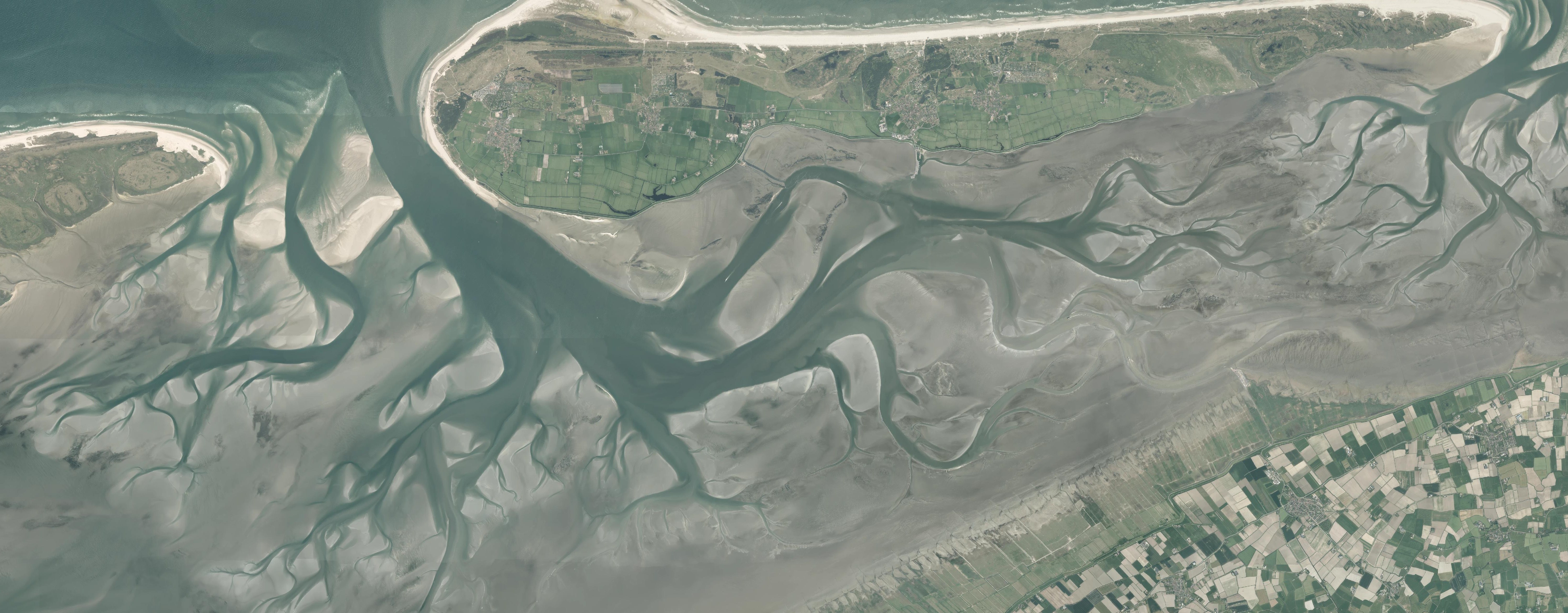
Kleinhans, van Kreveld, Ophelders, Sonke, Speckmann, and Verbeek [16] were the first to propose a method that computes networks for braided rivers and estuaries based on bathymetry. Their algorithm constructs the network from a set of (partially overlapping) low paths through the DEM (a striation), which ensures that bifurcations and confluences can be represented. There are many possible low paths and corresponding channels. The authors choose significant channels based on a morphological concept: sediment volume. Two channels can be considered similar if the volume of terrain between the channels is small, modeling the fact that a small volume of sediment can easily be eroded in a short time by water flow, merging the two channels into one [14]. The algorithm hence selects a subset of the striation paths which are separated by sufficient volume of sediment (see Figure 2). This method has two drawbacks. First and foremost, it is unstable with respect to minor changes of the terrain (see Figure 3). Secondly, in low-relief terrains, such as intertidal zones and estuaries, there are many geomorphologically significant dead-end channels (fingers), caused by tidal in- and outflow (see Figure 1 and its “tree of fingers”). Striation paths by design flow from one side of the terrain to the other and hence the method fails to detect fingers.
In this paper we retain the notion of volume-separated channels, but turn to persistence and discrete Morse theory to avoid instability. Specifically, we use the concept of volume persistence, which considers only those topological features of the DEM that correspond to “sand bars” of sufficient volume. That is, we use a volume-simplified DEM, which we obtain by pruning topological features of the terrain that can be eliminated by removing only a small amount of volume. Topological persistence was introduced by Edelsbrunner, Letscher, and Zomorodian [7], and is a record of homological changes throughout a filtration of an underlying space. Such filtrations are often defined with respect to the distance between points, however, other measures can be used. Carr, Snoeyink, and van der Panne [4] describe a method to simplify contour trees using so-called local geometric measures, such as (in 2D terrains) the line length of the contour, the area enclosed by the contour, or the volume of the enclosed region. This last type of filtration is exactly the one we use. The remaining channels in our volume-persistent network separate regions of the terrain with high significance.
A couple of years ago, a geomorphologcial paper [23] sketched how to use volume persistence to compute networks from bathymetry; however, the exposition lacks mathematical detail. Height persistence has previously been employed to fill local minima in terrains [5]. De Floriani, Iuricich, Magillo, and Simari [6] compared watershed methods and discrete Morse theory for the construction of watersheds, but only on terrains with high relief and water flow that follows steepest descent.
Contribution and organization.
In this paper we give a mathematically sound formalization of volume persistence and its use for network computation. In Section 2 we provide background on discrete Morse theory. Section 3 describes our method to construct a network based on volume persistence. By design these networks are stable under perturbations of small volume, however, like the channels that stem from striations, they connect one side of the terrain to the other. In Section 4 we develop the additional theory necessary to detect salient fingers. The major challenge here is to characterize the area and corresponding terrain volume that defines a finger. It is clear which area lies between two channels that first bifurcate and then merge again. Correspondingly, it is straightforward to compute the volume of terrain between two channels. But what area determines a finger? When are two fingers similar? Which fingers should be retained in a network given a volume threshold for persistence? To address these challenges, we introduce the notion of “spurs” on the terrain and define salient fingers as those that bound spurs of sufficient volume. Finally, in Section 5 we showcase the results of our method as implemented in our tool TopoTide (https://github.com/tue-alga/topotide).
2 Preliminaries
Our network extraction methods are grounded in discrete Morse theory and concepts from topology are useful to describe them. Additionally, various notions of volume play a central role in our methods. Therefore, in this section, we provide definitions related to these topics.
Discrete Morse theory.
Traditional Morse theory enables us to study a manifold by defining a Morse function, a differentiable function on the manifold, and studying its features such as critical points and stable and unstable manifolds. As the data describing our terrain is not continuous, but consists of discrete points, we assume the terrain is a two-dimensional cell complex : a surface defined by a set of zero-, one-, and two-cells so that the intersection of any two cells in is in itself. We then turn to discrete Morse theory [11, 20].
For cells and , we say that is a face of (or is a coface of ) if , and we say that is a facet of (or is a cofacet of ) if is a face of and . A discrete Morse function (DMF) is a map such that every cell has a lower (higher) value than its cofacets (facets) with at most one exception. It may be helpful to visualize as pairing facets to cofacets where these exceptions occur, in an analog to gradient flow from the smooth setting. These pairings are called gradient pairs and we may illustrate them using arrows pointing from facets to cofacets, as in Figure 4. A cell is critical if is not paired with any of its facets or cofacets. A critical zero-cell is called a minimum, a critical one-cell is called a saddle, and a critical two-cell is called a maximum.
Given a DMF , an ascending path is a sequence that alternates between zero- and one-cells, “swimming upstream” along the pairings induced by . Similarly, a descending path is a sequence that alternates between two- and one-cells, following the pairings induced by . The union of all ascending paths forms a spanning forest, and so does the union of all descending paths; these spanning forests are dual, with the exception of saddles. For each facet of a saddle, there exists a unique ascending path ending at that zero-cell and originating at a minimum; we define the ascending Morse–Smale complex (or MS-complex for brevity) as a graph with nodes corresponding to the minima of , and arcs corresponding to the pairs of ascending paths connected via saddles between them. See Figure 4. Similarly, for each cofacet of a saddle, there is a unique descending path ending at that two-cell and originating at a maximum. Note that, while a node corresponds to a zero-cell, an arc represents the union of potentially many zero- and one-cells. Furthermore, the highest zero-cell along is the highest facet of its saddle. Each face of contains a single maximum. For a subset , we write to denote the arc-induced subgraph on , i.e., the graph containing only the arcs and their endpoints.
Terrain data.
The input to our methods is a digital elevation model (DEM), a set of points and associated elevations. These points and elevations correspond to the elevations of geographic locations in a real-world or simulated terrain. DEMs come in many varieties, for instance triangular irregular networks (TINs) or other point configurations. In this paper, we suppose our DEM data consists of a regular rectilinear grid of measurement points. However, we emphasize that discrete Morse theory along with many of the methods we describe, generalizes to a wide variety of DEM types and structures.
We assume that our input DEM corresponds to a region homeomorphic to a disk, i.e., there are no arches or more complex structures. If any two zero-cells have identical elevation, we perform a slight perturbation so that general position is satisfied [8]. We add three additional zero-cells to an input DEM. First, we add two zero-cells at elevation to represent a global source and sink, and connect to the appropriate regions of the DEM (conceptually, the source and sink along this boundary). We then add a zero-cell at elevation to represent the land that is not part of the terrain of interest (e.g., the bank of a river), which we assign elevation , and connect to the entire (new) boundary, including the minimum points. Thus, is topologically a sphere (see Figure 5). Note that contains non-square two-cells adjacent to the infinite points, so does not have an entirely grid-like structure; however, the region of interest, namely, points that correspond to data measurements, is endowed with a grid structure, and it suffices to conceptualize as cubulated. We call a DEM adapted in this way a terrain, which is the starting point for our work.
Choosing a discrete Morse function.
A discrete Morse function (DMF) assigns a real value to every cell of : not only the zero-cells, but also the one- and two-cells. On the other hand, our terrain data consists of elevation values for the zero-cells of , but not the one- and two-cells. Thus, we have to extend these measurements on the zero-cells to every cell of in such a way that we obtain a discrete Morse function, whose critical points and gradient pairs reflect the input measurements. Several choices have been proposed in the literature, see for example [21, 12, 13, 9, 22, 19, 10]. In this paper we use the method proposed in [22]; we sketch the relevant gradient pairings in the following construction.
Construction 1 (From Elevations to Pairings).
The real values associated to every zero-cell in a terrain induce a high-to-low lexicographical order on all cells. First, pair every zero-cell with its lowest lower cofacet, if it exists. Next, for every remaining one-cell , consider the cofacets of for which is the highest facet. Among these, pair with the two-cell for which the one-cell opposite is lowest. Finally, repeat the previous step for every remaining one-cell , considering the unpaired cofacets of for which is the second-highest facet.
A main contribution of [22] shows the gradient pairings described above are valid, and do not contradict given elevation data.
Lemma 2 (Adapted from [22]).
Let be a terrain. Then the pairings of Construction 1 correspond to a valid DMF on , where, for all zero-cells , is the elevation of .
Since a set of valid gradient pairings is equivalent to a DMF inducing those pairings, we generally proceed by discussing gradient pairings rather than an explicit function.
Volume and Paths.
Our filtrations depend on a volume-based parameter. Thus, we first need to define the volume of a region in . Conceptually, we think of the elevation of each zero-cell as volume being divided among its four adjacent two-faces, so that each zero-cell contained in a region contributes zero, one, two, three, or four quarters of its volume (height value) to the total, depending on how many of its adjacent two-faces are in the region.
Definition 3 (Quarter-Pillar Volume).
Consider some height and two-cell . Denote the zero-cells adjacent to by , and , and for , let denote the elevation of . Then we define the volume of above as
That is, each zero-cell contributes a quarter of its elevation above to the volume of . Next, let . We define the volume of as the sum of volumes of all two-cells contained in .
Note that Definition 3 could easily be adapted for more general settings, e.g., if faces do not necessarily have exactly four nodes, or if the size or shape of the faces is salient. We want to know the volume of regions of the terrain that are above a particular elevation, but as elevation is only defined on zero-cells, we introduce the following concept.
Definition 4 (Zero-Cell Superlevel Set).
Given a zero-cell of some terrain , the zero-cell superlevel set of is the collection of zero-cells of with equal or higher elevation than .
We are generally interested in measuring volumes that correspond to continuous regions of the terrain. This is formalized in the following definition.
Definition 5 (Zero-Cell Connected).
Let be a set of zero-cells. Two zero-cells are (zero-cell) connected if and only if there is a sequence such that, for , every is contained in and every adjacent pair, and , are faces of a common two-cell of . We say that is (zero-cell) connected if every pair of zero-cells in is zero-cell connected. A connected component of is a connected set that is not a proper subset of any other connected set in .
Next, we introduce an idea that allows us to consider lexicographically lowest paths.
Definition 6 (Lexicographic Order of Paths).
In a terrain , let and be paths of alternating zero- and one-cells. Then we say is lexicographically lower than if the list of zero-cells in sorted by elevation from high to low is lexicographically lower than the sorted list of zero-cells in .
Roughly speaking, Construction 1 defines ascending paths of an MS-complex by introducing zero-/one-cell pairings that are lexicographically low. This has the following consequence.
Corollary 7 (Lowest Paths are Arcs of ).
Suppose that is a terrain with a DMF defined as in Construction 1, and consider two minima, and . Then the lexicographically lowest path through zero- and one-cells of connecting and corresponds to arcs of the corresponding MS-complex, .
3 Volume Persistence for Braided Rivers and Estuaries
In this section, we detail our network extraction method when the terrain in question is a braided river or estuary in which no channels truncate (i.e., there are no degree one nodes in the network).
In practice, terrains corresponding to actual data are quite noisy, so a network that is simply the MS-complex for some corresponding DMF is much more complex than what we might want. Thus, we filter based on a volume parameter. Conceptually, we want to keep channels that run between two “hills” that contain enough volume. Note that if an arc ends at a minimum in a shallow basin, an endpoint of may have degree one, i.e., does not separate two hills. We specify arcs that separate hills more formally below.
Definition 8 (Splitting Arcs).
Let be the MS-complex for a DMF on a terrain . For an arc , let denote the highest zero-cell of contained in . Let denote the connected component of the zero-cell superlevel set at the height of that contains . We say that is a splitting arc if is two connected components.
Next, we assign a volume to each splitting arc, corresponding to the volume of sediment that would need to be removed in order for the channel to no longer be defined.
Definition 9 (Volume Persistence of Splitting Arcs).
Let be the MS-complex for a DMF on a terrain . For a splitting arc , let denote the highest zero-cell of in . Let be the connected component of the zero-cell superlevel set at the height of that contains . Let and be the two connected components of . Finally, let (and ) be the set of two-cells that have at least one incident zero-cell in (and , respectively). We define the volume persistence of as the minimum volume of or .
See Figure 6. If the volume persistence of an arc is low, a small change to the terrain would remove the arc. Thus we use the volume persistence of arcs to filter , as follows.
Definition 10 (Volume-Filtered Subnetwork).
For the MS-complex of a terrain , and for , let be the graph induced by the set of splitting arcs with volume persistence at least , along with all (remaining) lowest paths between nodes in .
Note that by Corollary 7, the lowest path between a pair of minima is made up of arcs of , which may be splitting or non-splitting. The following lemma asserts that using as a parameter defines a filtration of , where inclusion occurs as decreases.
Lemma 11.
Let be an MS-complex for a terrain , and let such that . Then .
Proof.
Consider a splitting arc . Then the volume persistence of is greater than or equal to , meaning . Since our choice of was arbitrary, every splitting arc of is a splitting arc of , and . Then the lowest paths between two nodes of are also in . Thus, .
We also take the following general position assumptions. Let be a DMF of a terrain . We assume is injective on the zero-cells of with a finite height, i.e., they each have a unique height. Furthermore, given , the MS-complex associated to , each arc of has a unique volume persistence in the sense of Definition 9.
3.1 Properties of Merging Faces
Given a DMF over a terrain and the associated MS-complex , our goal is now to produce the volume-filtered subnetwork for any . The computational challenge is to efficiently compute the volume persistence of each splitting arc . Recall that, for the highest zero-cell of along , the volume persistence of is the minimum volume of a connected component of the superlevel set above and on either side of , so we first need to identify such components. A naïve approach might be to begin at a saddle one-cell and use a depth-first search method to explore neighboring two-cells, adding them to the connected components for until we identify a boundary made up of cells with lower height, i.e., the boundary of the relevant connected components of the superlevel set. However, in doing so, we would potentially revisit the cells in the highest face of times (where is the number of saddles), cells in the second highest face times, and so on. Instead, we propose a faster method to find relevant superlevel sets that makes use of containment properties. By processing arcs “from high to low,” we can use information about previously explored regions and avoid the need to analyze the same two-cells more than once. More formally, the following lemma establishes a helpful property that is a result of this strategy.
Lemma 12.
Let be the MS-complex of a DMF on a terrain with gradient pairings as in Construction 1. Let be the total ordering of the arcs from high to low via their highest zero-cell. For , let denote the highest zero-cell of . Then the connected component of all zero-cells in the superlevel set above and containing is strictly contained in the faces of the graph that are adjacent to .
Proof.
For some , let denote the highest zero-cell of along arc , and let denote the zero-cell connected component of the superlevel set above and containing (i.e., the zero-cells in the hills above ). Let denote the union of the faces of adjacent to , considered as a collection of zero-, one-, and two-cells.
First, suppose the boundary of does not contain . Then arcs in the boundary of all have a highest zero-cell lower than the height of . In particular, all zero-cells contained in the boundary of have lower elevation than , and are therefore not contained in . Then any connected collection of zero-cells of may not cross the boundary of . By construction, intersects at the single point , an interior point of , so clearly is not disjoint from . Thus, , as desired.
In the case that the boundary of contains (for instance, if has a node with degree one), the boundary of is comprised of a set of arcs whose collective highest zero-cell is . Then the only way for a connected collection of zero-cells in to leave is through . However, is not an endpoint of (endpoints of are local minima), so all zero-cells neighboring with higher elevation must be in the interior of , and the claim follows by similar logic to the preceding case.
Finally, we aim to show that the behavior of zero-cell connectivity of superlevel sets mimics behavior in a continuous terrain; namely, all points in the superlevel set above an arc contained in a face of are part of the same zero-cell connected component.
We first establish a helpful lemma for , before any arcs have been removed.
Lemma 13.
Let be the MS-complex of a DMF on a terrain , with gradient pairings as in Construction 1. Let denote the highest zero-cell along the boundary of some face of . Then the connected component of the superlevel set of contains both and the highest zero-cell of the maximum in that face.
Proof.
Recall that each maximum is contained in a distinct face of . Let denote the highest zero-cell along the boundary of some face of . The saddle containing is the face of some two-cell, which we denote . Since the union of descending paths in a face of forms a spanning tree, there is a unique path from to the maximum, following gradient pairs up (i.e., a path of alternating paired one- and two-cells).
For any gradient pair from a one-cell to a two-cell , we claim that the highest zero-cell of is also a zero-cell of . Recall from Construction 1 that can be paired with only if is lexicographically either the highest or second-highest one-cell of . In both cases, the highest zero-cell is necessarily a face of . Thus, by following , we obtain a non-decreasing path of zero-cells from to the highest zero-cell of the maximum.
Using Lemma 13, we now show that particular superlevel sets contained in faces of (i.e., without the first highest arcs) are connected. Importantly, this means intuition about superlevel sets from a continuous terrain also applies in our discretized setting.
Lemma 14.
Let be the MS-complex of a DMF a terrain , with gradient pairings as in Construction 1. Let be the total ordering of the arcs from high to low via their highest zero-cell. For , let denote the highest zero-cell of . Then the zero-cells of the superlevel set at contained in a face of the graph adjacent to form a single zero-cell connected component.
Proof.
For some , consider the graph . Let denote a face of adjacent to , let denote the highest zero-cell along , and let denote the superlevel set at the height of that is contained in . First, we observe that any connected component of has some zero-cell with maximum height, and so is adjacent to at least one maximum. We therefore aim to show all maxima in that are adjacent to zero-cells of (i.e., the maxima of that are “in” the superlevel set) are connected in . By Lemma 13, we know that any two such maxima are in the same connected component of the superlevel set of , where is the highest zero-cell of the arc that separates these maxima in . However, such a zero-cell is interior to , which means must be higher than , otherwise, the arc would not have been removed in , and the arc would be a boundary of . This means maxima in adjacent to a zero-cell of are connected in , and we have shown the claim.
For a single two-cell , consider the function for volume in above a particular height; as the height increases/decreases, the volume changes according to a piecewise linear function, with discontinuities every time the height passes over one of the zero-cells of . Thus, we have a piecewise linear function associated to each two-cell in the terrain.
The function for volume under a face of above some height is then simply the sum of functions for each two-cell of the face. If the parameters at which the volume function for the face of changes are sorted (i.e., if the heights of zero-cells in the face are sorted), we can query the function at a specific height by using binary search on the parameters in time. By Lemma 12, by processing arcs from high to low, we know exactly which faces are in the relevant components of the superlevel set above some arc; it is the adjacent merges of faces after we remove all higher arcs from . The function for volume after the merge of two faces is the sum of functions for volume in each face individually.
4 Volume Persistence for Intertidal Zones
We shift our attention to the detection of fingers, which is primarily relevant when analyzing intertidal zones. As before, we assume our input is a terrain and use Construction 1 to identify gradient pairings corresponding to a compatible DMF. One major difference between detecting bars separating channels (Section 3) and detecting fingers is that fingers are not necessarily arcs of the MS-complex. Therefore, we have to search for fingers inside each face of the MS-complex. We thus first apply the method from Section 3 for some fixed to identify channels from the MS-complex that separate “sufficient volume.” These remaining channels divide the terrain into faces; our goal is to extract fingers within each such face.
First, we define an adaptation of descending paths. Recall that descending paths are alternating sequences of two- and one-cell gradient pairs that collectively form a spanning forest over the terrain, and each maximum corresponds to a tree in this forest. When we filter the MS-complex in Section 3, we remove entire arcs, so that multiple maxima are contained within the same region. Thus, just as we included saddles to connect ascending paths in Section 3, we include saddles to connect descending paths within a particular region. This is illustrated in Figure 7 and defined formally below.
Definition 15 (Red Tree).
For a terrain, , and , let denote the associated volume-filtered subnetwork. Within a face of , add saddles from high to low to the union of descending paths contained within a face of , stopping once the set of initial trees is joined to form a single (spanning) tree, and omitting any saddles whose inclusion would form a cycle. We call this merged collection of descending paths and saddles a red tree.
Volume and Height Filtration of Descending Paths.
In Section 3, we associate volumes to splitting arcs of , based on the minimum volume of either of the two hills that the arc separates. Here, we take a finer-grained approach and, instead, associate volume to individual one-cells in a red tree. While a one-cell generally does not separate hills like a splitting arc of does, we take inspiration from this sort of behavior and instead, consider the volumes of the two subtrees formed by the one-cell’s removal, above a given height. Note that it makes sense to discuss “volume of a subtree” in this setting, as the subtrees are collections of two- and one-cells, and thus, the quarter pillar volume (Definition 3) may be nonzero. More formally, we have the following.
Definition 16 (Volume of a One-Cell for Height ).
Let be a red tree with one-cells . We define the volume function at any fixed height , as follows. For a one-cell , let be the subforest of whose one-cells are each incident to some zero-cell with height at least . Let and denote the two subtrees of adjacent to . Let and be the volumes of the part of the superlevel set of that corresponds to and , respectively. Then we define .
See Figure 8. If the volume of a one-cell at a particular height is low, it does not represent a location in the terrain with significant “separation.” Since we eventually use the structure of one-cells that do have significant separation in order to identify the locations of our finger channels, we filter the red tree in the following way.
Definition 17.
For , consider , a volume-filtered subnetwork for some terrain. Suppose that is a red tree corresponding to . Let denote the set of one-cells of . Then, for , we define
Note that we now have both a volume and height parameter. If varies within a range that does not change the volume filtered subnetwork, , then decreasing or means more one-cells become part of , i.e., we have a bifiltration. However, if varies within a range such that changes, we are no longer guaranteed this property. In particular, if increases and an arc of is removed, two previously disconnected red trees merge, potentially causing the involved one-cells to have a jump in their volumes. In other words, one-cells are monotonically included only within intervals of for which does not change.
Identifying Significant Spurs.
First, we define a spur, which is a structure defined for a fixed volume parameter and, conceptually, is determined by noting the order in which various red one-cells have sufficient volume as height varies. It may be helpful to recall that is a tree made up of one- and two-cells.
Definition 18 (Spurs).
Let be a red tree. For a fixed , each one-cell of has a height above which it has volume at least ; call this the significance of . Let be a leaf of ; we check if its adjacent one-cell itself has exactly one adjacent one-cell with higher significance; if so, we move to this new one-cell and repeat this process. Once we encounter a one-cell that does not have exactly one adjacent one-cell with higher significance, we note its last two-cell, , and define a spur with top and bottom , which is the entire subtree of rooted at containing the path from to . We identify all other spurs by repeating this process for every leaf one-cell of .
See Figure 9. The following lemma gives us insight into the structure of spurs of .
Lemma 19.
Let be a red tree with leaves, and, for a fixed volume , let denote the set of spur top and bottom pairs. Then, for if the paths from to and to intersect, the intersection contains either or .
Proof.
When , the claim holds trivially. Then consider some and suppose that the path from to intersects the path from to , i.e., there is some last two-cell, , contained in both paths. Towards a contradiction, suppose is not either or . Then we can denote and as the one-cells on the path from to just before and just after respectively: define and similarly. Since is the last two-cell in the intersection, .
Without loss of generality, suppose the significance of is no higher than that of . Note that and are both adjacent to , and only can have a higher significance than , otherwise, would be adjacent to , contradicting . But then both and would have higher significance than , contradicting that is not adjacent to .
Since a spur is a connected collection of one- and two-cells, we measure the volume of a spur using quarter-pillar volume, just as we did previously for other types of superlevel sets.
Definition 20 (Volume Persistence of Spurs).
Let be a spur and suppose that the highest zero-cell adjacent to a cell of has height . We say that the volume persistence of is the volume of the superlevel set at height contained in .
A spur with volume persistence of at least corresponds to a region of the terrain with enough volume to separate a channel on either side of it, at least up to its flanking height. Specifically, we place fingers along the boundaries of spurs, defined below.
Definition 21 (Spur Boundaries).
Consider a spur, . We refer to the collection of zero- and one-cells of that are adjacent to some two-cell not in the boundary of .
We choose fingers that lie on spur boundaries; our final lemma helps justify this choice.
Lemma 22.
Let be a spur with top . Then all zero- and one-cells on the boundary of that are not adjacent to lie on some collection of ascending paths and saddles.
Proof.
Suppose, towards a contradiction, that is a one-cell in the boundary of , not adjacent to , that does not lie on an ascending path or saddle of the terrain. Recall that every one-cell is either part of an ascending path, is a saddle, or is part of a descending path. I.e., it must be that is part of a descending path, and thus has a gradient pair to some adjacent two-cell, . But, since is the entire subtree below its top, we have , which contradicts our assumption that is on the boundary of .
Intertidal Network Computation.
We are now ready to compute fingers. We summarize our entire procedure as follows:
-
1.
Extend given elevation data to a DMF on all cells (Construction 1).
-
2.
Compute , i.e., channels that separate hills of volume no less than (Section 3), for an appropriate choice of (in practice, this value is determined by domain experts).
-
3.
In each face of , create a red tree (Definition 15).
-
4.
For such a red tree, determine its set of spurs (Definition 18).
-
5.
Consider the subset, , of spurs with volume persistence no less than (Definition 20).
-
6.
For each spur , consider the two walks (clockwise and counterclockwise) around the boundary of starting at the top of . In each direction, note the first zero-cell we encounter with height no more than the flanking height of . Such zero-cells define the degree-one end of a finger, and we complete the finger by flowing down via the lowest lexicographical path (along the boundary of , and then possibly through additional ascending paths and saddles) until we reach a minimum of .
-
7.
Output along with all fingers as the resulting network.
We end with a remark that highlights connections between this section and Section 3.
Remark 23.
We present intertidal network computation within a face of and the methods for computing (Section 3) as two separate operations, but the outputs for each actually share many fundamental behaviors in relation to the terrain. Namely, suppose we consider faces of as a variant of a spur. The maximum height at which such a face has volume no less than is at the highest zero-cell along its boundary, which is necessarily the zero-cell of some saddle. That is, this highest zero-cell height behaves like the flanking height for a spur. Then, just as in Step of the intertidal network computation procedure, by flowing down from this zero-cell (this time in two directions) via the lowest lexicographical path to a minimum of some other face, we recover as a network. Thus, we could think of network computation in a more streamlined way, and not differentiate between types of ascending paths. However, we chose to present the computation of as a filtration of channels for clarity, as well as to connect better with related work.
5 Implementation and Validation
To validate our modeling, we implemented our methods and tested the implementation using two real-world datasets: a DEM of the Western Scheldt estuary, and a DEM of a part of the Wadden Sea. The first dataset serves to demonstrate the network extraction from Section 3, while the second dataset demonstrates the finger extraction from Section 4.
Western Scheldt.
Figure 10 shows the input and output for the Western Scheldt dataset. In the resulting network (Figure 10f) the color of each arc encodes its volume persistence: from dark purple (high volume) to bright pink (low volume). Arcs with volume persistence less than are not shown.
In practice, we found that the method is quite stable under small changes in the DEM. To demonstrate this stability, in Figure 11 we show the networks extracted from historical DEMs from 1999, 2004, 2009, and 2014. Though some areas of the estuary underwent rapid changes during this period, the other parts of the extracted network stay similar.
Wadden Sea.
Figure 12 shows the input and output for the Wadden Sea dataset. This dataset spans the same area as depicted in Figure 1. Figure 12b shows the result of our network extraction method. The method detects one significant bar between two channels, but as expected, does not detect the other features, as they are all fingers. Figure 12d then shows the result of our finger extraction method. The spurs (Figure 12c) represent areas of sufficient volume between fingers, and the extracted fingers capture the tree-like structure of the tidal basin well. In most cases, the flanking height of each spur is a good choice for determining how high the starting point of each finger lies. However, some of the extracted fingers are very short because the flanking height is quite low. This may be alleviated by filtering out fingers in their entirety if their length is below a given threshold.
Conclusion.
The networks found by the implementation show that our algorithm is indeed able to identify geomorphologically salient networks, including fingers, in low-relief terrains. Domain experts have confirmed the high quality of the networks and thereby validated our mathematical modeling.
References
- [1] L. Arge, J. S. Chase, P. Halpin, L. Toma, J. S. Vitter, D. Urban, and R. Wickremesinghe. Efficient flow computation on massive grid terrain datasets. GeoInformatica, 7(4):283–313, 2003. doi:10.1023/A:1025526421410.
- [2] M. de Berg, P. Bose, K. Dobrint, M. van Kreveld, M. Overmars, M. de Groot, T. Roos, J. Snoeyink, and S. Yu. The complexity of rivers in triangulated terrains. In Proc. 8th Canadian Conference on Computational Geometry (CCCG), pages 325–330, 1996. doi:10.1515/9780773591134-057.
- [3] M. de Berg, O. Cheong, H. Haverkort, J. Lim, and L. Toma. The complexity of flow on fat terrains and its I/O-efficient computation. Computational Geometry, 43(4):331–356, 2010. doi:10.1016/j.comgeo.2008.12.008.
- [4] H. Carr, J. Snoeyink, and M. van de Panne. Simplifying flexible isosurfaces using local geometric measures. In Proc. 15th IEEE Visualization Conference (VIS), pages 497–504, 2004. doi:10.1109/VISUAL.2004.96.
- [5] A. Danner, T. Mølhave, K. Yi, P. K. Agarwal, L. Arge, and H. Mitasova. TerraStream: From elevation data to watershed hierarchies. In Proc. 15th Annual ACM International Symposium on Advances in Geographic Information Systems (GIS), 2007. doi:10.1145/1341012.1341049.
- [6] L. De Floriani, F. Iuricich, P. Magillo, and P. Simari. Discrete Morse versus watershed decompositions of tessellated manifolds. In Proc. 17th Image Analysis and Processing (ICIAP), pages 339–348, 2013. doi:10.1007/978-3-642-41184-7_35.
- [7] H. Edelsbrunner, D. Letscher, and A. Zomorodian. Topological persistence and simplification. Discrete Computational Geometry, 28:511–533, 2002. doi:10.1007/s00454-002-2885-2.
- [8] H. Edelsbrunner and E. P. Mücke. Simulation of simplicity: A technique to cope with degenerate cases in geometric algorithms. ACM Transactions on Graphics, 9(1):66–104, 1990. doi:10.1145/77635.77639.
- [9] B. T. Fasy, B. McCoy, and D. L. Millman. If you must choose among your children, pick the right one. In Proc. 32nd Canadian Conference on Computational Geometry (CCCG), pages 336–344, 2020.
- [10] R. Fellegara, F. Luricich, L. De Floriani, and K. Weiss. Efficient computation and simplification of discrete Morse decompositions on triangulated terrains. In Proc. 22nd ACM SIGSPATIAL International Conference on Advances in Geographic Information Systems, pages 223–232, 2014. doi:10.1145/2666310.2666412.
- [11] R. Forman. A user’s guide to discrete Morse theory. Séminaire Lotharingien de Combinatoire, 48(B48c):1–35, 2002.
- [12] A. Gyulassy, P.-T. Bremer, B. Hamann, and V. Pascucci. A practical approach to Morse–Smale complex computation: Scalability and generality. IEEE Transactions on Visualization and Computer Graphics, 14(6):1619–1626, 2008. doi:10.1109/TVCG.2008.110.
- [13] H. King, K. Knudson, and N. Mramor. Generating discrete Morse functions from point data. Experimental Mathematics, 14(4):435–444, 2005. doi:10.1080/10586458.2005.10128941.
- [14] M. G. Kleinhans. Flow discharge and sediment transport models for estimating a minimum timescale of hydrological activity and channel and delta formation on Mars. Journal of Geophysical Research, 110(E12), 2005. doi:10.1029/2005JE002521.
- [15] M. G. Kleinhans, R. I. Ferguson, S. Lane, and R. J. Hardy. Splitting rivers at their seams: Bifurcations and avulsion. Earth Surface Processes and Landforms, 38(1):47–61, 2013. doi:10.1002/esp.3268.
- [16] M. G. Kleinhans, M. van Kreveld, T. Ophelders, W. Sonke, B. Speckmann, and K. Verbeek. Computing representative networks for braided rivers. Journal of Computational Geometry, 10(1):423–443, 2019. doi:10.20382/jocg.v10i1a14.
- [17] W. A. Marra, M. G. Kleinhans, and E. A. Addink. Network concepts to describe channel importance and change in multichannel systems: Test results for the Jamuna River, Bangladesh. Earth Surface Processes and Landforms, 39(6):766–778, 2014. doi:10.1002/esp.3482.
- [18] P. Passalacqua, S. Lanzoni, C. Paola, and A. Rinaldo. Geomorphic signatures of deltaic processes and vegetation: The Ganges-Brahmaputra-Jamuna case study. Journal of Geophysical Research, 118:1838–1849, 2013. doi:10.1002/jgrf.20128.
- [19] V. Robins, P. J. Wood, and A. P. Sheppard. Theory and algorithms for constructing discrete Morse complexes from grayscale digital images. IEEE Transactions on Pattern Analysis and Machine Intelligence, 33(8):1646–1658, 2011. doi:10.1109/TPAMI.2011.95.
- [20] N. A. Scoville. Discrete Morse Theory, volume 90. American Mathematical Society, 2019.
- [21] N. Shivashankar, Senthilnathan M., and V. Natarajan. Parallel computation of 2D Morse–Smale complexes. IEEE Transactions on Visualization and Computer Graphics, 18(10):1757–1770, 2012. doi:10.1109/TVCG.2011.284.
- [22] N. Shivashankar and V. Natarajan. Parallel computation of 3D Morse–Smale complexes. Computer Graphics Forum, 31(3):965–974, 2012. doi:10.1111/j.1467-8659.2012.03089.x.
- [23] W. Sonke, M. G. Kleinhans, B. Speckmann, W. M. van Dijk, and M. Hiatt. Alluvial connectivity in multi-channel networks in rivers and estuaries. Earth Surface Processes and Landforms, 47(2):477–490, 2022. doi:10.1002/esp.5261.
- [24] A. Tejedor, A. Longjas, I. Zaliapin, and E. Foufoula-Georgiou. Delta channel networks: 1. A graph-theoretic approach for studying connectivity and steady state transport on deltaic surfaces. Water Resources Research, 51(6):3998–4018, 2015. doi:10.1002/2014WR016577.
- [25] A. Tejedor, A. Longjas, I. Zaliapin, and E. Foufoula-Georgiou. Delta channel networks: 2. Metrics of topologic and dynamic complexity for delta comparison, physical inference, and vulnerability assessment. Water Resources Research, 51(6):4019–4045, 2015. doi:10.1002/2014WR016604.
- [26] S. Yu, M. van Kreveld, and J. Snoeyink. Drainage queries in TINs: from local to global and back again. In Advances in GIS Research II: Proc. 7th International Symposium on Spatial Data Handling, pages 829–842, 1997.