Efficient Greedy Discrete Subtrajectory Clustering

Abstract
We cluster a set of trajectories using subtrajectories of . We require for a clustering that any two subtrajectories in a cluster have disjoint intervals and . Clustering quality may be measured by the number of clusters, the number of vertices of that are absent from the clustering, and by the Fréchet distance between subtrajectories in a cluster.
A -cluster of is a cluster of subtrajectories of with a centre , where all subtrajectories in have Fréchet distance at most to . Buchin, Buchin, Gudmundsson, Löffler and Luo present two -time algorithms: SC(, , , ) computes a single -cluster where has at least vertices and maximises the cardinality of . SC(, , , ) computes a single -cluster where has cardinality and maximises the complexity of .
In this paper, which is a mixture of algorithms engineering and theoretical insights, we use such maximum-cardinality clusters in a greedy clustering algorithm. We first provide an efficient implementation of SC(, , , ) and SC(, , , ) that significantly outperforms previous implementations. Next, we use these functions as a subroutine in a greedy clustering algorithm, which performs well when compared to existing subtrajectory clustering algorithms on real-world data. Finally, we observe that, for fixed and , these two functions always output a point on the Pareto front of some bivariate function . We design a new algorithm PSC(, ) that in time computes a -approximation of this Pareto front. This yields a broader set of candidate clusters, with comparable quality to the output of the previous functions. We show that using PSC(, ) as a subroutine improves the clustering quality and performance even further.
Keywords and phrases:
Algorithms engineering, Fréchet distance, subtrajectory clusteringFunding:
Ivor van der Hoog: This project has received funding from the European Union’s Horizon 2020 research and innovation programme under the Marie Skłodowska-Curie grant agreement No 899987Copyright and License:
2012 ACM Subject Classification:
Theory of computation Computational geometrySupplementary Material:
Software (Source code): https://github.com/laraost/DiscreteSubtrajectoryClustering
archived at
archived at
Funding:
Ivor van der Hoog, Eva Rotenberg, and Daniel Rutschmann are grateful to the Carlsberg Foundation for supporting this research via Eva Rotenberg’s Young Researcher Fellowship CF21-0302 “Graph Algorithms with Geometric Applications”.Editors:
Oswin Aichholzer and Haitao WangSeries and Publisher:
1 Introduction
Trajectories describe the movement of objects. The moving objects are modeled as a sequence of locations. Trajectory data often comes from GPS samples, which are being generated on an incredible scale through cars, cellphones, and other trackers. We focus on subtrajectory clustering where clusters are sets of subtrajectories. The goal is to create few clusters and to ensure that subtrajectories within a cluster have low pairwise discrete Fréchet distance. This algorithmic problem has been studied extensively [1, 8, 10, 12, 13, 15, 16, 19, 21, 22, 20, 24, 27, 30] in both theoretical and applied settings. For surveys, see [7] and [28].
Subtrajectory clustering.
Comparing whole trajectories gives little information about shared structures. Consider two trajectories and that represent individuals who drive the same route to work, but live in different locations. For almost all distance metrics, the distance between and is large because their endpoints are (relatively) far apart. However, and share similar subtrajectories. Subtrajectory clustering allows us to model a wide range of behaviours: from detecting commuting patterns, to flocking behaviour, to congestion areas [12]. In the special case where trajectories correspond to traffic on a known road network, trajectories can be mapped to the road network. In many cases, the underlying road network might not be known (or it may be too dense to represent). In such cases, it is interesting to construct a sparse representation of the underlying road network based on the trajectories. The latter algorithmic problem is called map construction, and it has also been studied extensively [2, 6, 3, 14, 17, 25, 26]. We note that subtrajectory clustering algorithms may be used for map construction: if each cluster is assigned one centre, then the collection of centres can be used to construct an underlying road network [9, 10].
Related work.
BBGLL [12] introduce the following problem. Rather than clustering , their goal is to compute a single cluster. Given , a -cluster is any pair where:
-
is a subtrajectory of a trajectory in ,
-
is a set of subtrajectories, where for all , ,
-
and, for all , the Fréchet distance between and is at most .
See Figure 1. They define two functions that each output a single -cluster :
-
SC(, , , ) requires that and maximises .
-
SC(, , , ) requires that and maximises .
If and , their algorithms use time and space.
AFMNPT [1] propose a clustering framework. They define a clustering as any set of clusters. They propose a scoring function with constants that respectively weigh: the number of clusters, the radius of each cluster, and the number of uncovered vertices. Their implement a heuristic algorithm that uses this scoring function.
BBDFJSSSW [9] do map construction. They compute a set of -clusters for various . For each , they use as a road on the map they are constructing. Thus, it may be argued that [9] does subtrajectory clustering. As a preprocessing step, they implement SC(, , , ). Choosing various and , they compute a collection of “candidate” clusters. They greedily select a cluster , add it to the clustering, and remove all subtrajectories in from all remaining clusters in . For a cluster , this may split a into two subtrajectories. BBGHSSSSSW [10] give improved implementations.
ABCD [4] do not require that for all , . They do require that the final clustering has no uncovered vertices, and that for each cluster , for some given . For any , denote by the minimum-sized clustering that meets their requirements. Their randomised polynomial-time algorithm computes a clustering of -clusters of size . BCD [8] give polynomial-time clustering algorithm of -clusters of size . Conradi and Driemel [16] implement an -time algorithm that computes a set of -clusters of size .
Contribution.
Our contribution is threefold. First, in Section 5, we describe an efficient implementation of SC(, , , ) and SC(, , , ). We compare our implementation to all existing single-core implementations.
In Section 5 we propose that SC(, , , ) produces high-quality clusters across all clustering metrics. We create a greedy clustering algorithm that fixes and iteratively adds the solution SC(, , , ) to the clustering (removing all vertices in from ). An analogous approach for SC(, , , ) gives two clustering algorithms.
In Section 6 we note that the functions SC(, , , ) and SC(, , , ) search a highly restricted solution space, having fixed either the minimum length of the centre of a cluster or the minimum cardinality. We observe that these functions always output a cluster on the Pareto front of some bivariate function . Since points on this Pareto front give high-quality clusters, we argue that it may be beneficial to approximate all vertices of this Pareto front directly – sacrificing some cluster quality for cluster flexibility. We create a new algorithm PSC(, ) that computes in time and space a set of clusters that is a -approximation of the Pareto font of . We show that using PSC(, ) as a subroutine for greedy clustering gives even better results.
In Section 7 we do experimental analysis. We compare our clustering algorithms to AFMNPT [1] and BBGHSSSSSW [10]. We adapt the algorithm in [10] so that it terminates immediately after computing the subtrajectory clustering. We do not compare to Conradi and Driemel [16] as their setting is so different that it produces incomparable clusters. We compare the algorithms based on their overall run time and space usage. We evaluate the clustering quality along various metrics such as the number of clusters, the average cardinality of each cluster, and the Fréchet distance between subtrajectories in a cluster. Finally, we consider the scoring function by AFMNPT [1].
2 Preliminaries
The input is a set of trajectories where . We denote by all vertices of . We view any trajectory with vertices as a map from to where is the ’th vertex on . For brevity, we refer to as a single trajectory obtained by concatenating all trajectories in arbitrarily. A boundary edge in is any edge in between the endpoints of two consecutive trajectories. A subtrajectory of is defined by with , where we require that the subcurve from to contains no boundary edge.
Fréchet distance.
We first define discrete walks for pair of trajectories and in . We say that an ordered sequence of points in is a discrete walk if consecutive pair have and . The cost of a discrete walk is the maximum distance over . The discrete Fréchet distance is the minimum-cost discrete walk from to :
Free-space matrix.
Given and a value , the Free-space matrix is an -matrix where for all the matrix has a zero at position , if . We use matrix notation where denotes row and column . In the plane, denotes the top left corner. We also use to denote the digraph where the vertices are all and there exists an edge from to whenever (see Figure 2):
-
and , and
-
.
Alt and Godeau [5] show that for any two subtrajectories and :
if and only if there is a directed path from to .
Definition 1.
Given and , we say that a vertex in ) can reach row if there exists an integer such that there is a directed path from to . We denote by the minimum integer such that can reach row .
Definition 2 (Figure 1).
A cluster is any pair where is a subtrajectory and is a set subtrajectories with . We require that for all , . We define its length , cardinality , and coverage S.
Note that we follow [1, 9, 10, 12] and consider only disjoint clusterings, meaning , , the intervals and are disjoint. For brevity, we say that a -cluster is any cluster where .
Definition 3.
A clustering is a set of clusters. Its coverage is .
AFMNPT [1] propose a cost function to determine the quality of a clustering . We distinguish between -centre and -means clustering:
Definition 4.
Given constants , is a sum that weights three terms:
-
1.
The number of clusters in : .
-
2.
The chosen cost function for the clustering. I.e.,
when doing -centre clustering, or
when doing -means clustering.
-
3.
The fraction of uncovered points: .
We also consider unweighted metrics: the maximal and average Fréchet distance between subtrajectories in a cluster, and the maximal and average cardinality of the clusters.
3 Data
We use five real-world data sets (see Table 1). For some of these data sets we include a subsampled version that only retains a fraction of the trajectories.
-
The fourth data set is the Drifter data set that was used for subtrajectory clustering by Driemel and Conradi [16]. It consists of GPS data from ocean drifters.
-
The fifth data set is the UnID data set, which is the smallest data set used in [29].
Unfortunately, we cannot use any of the data sets in [1]. Most of these are no longer available. Those that are available are far too large. It is unknown how [1] preprocessed these.
Synthetic data.
All competitor algorithms do not terminate on the larger real-world data sets, even when the time limit is 24 hours. Thus, we primarily use these sets to compare algorithmic efficiency. Our qualitative analysis uses the subsampled data sets and synthetic data. We generate data by creating a random domain . Then, for some parameter , we randomly select of the domain and invoke an approximate TSP solver. We add the result as a trajectory. This results in a collection of trajectories with many similar subtrajectories. Synthetic-A has a random domain of 200 vertices. Synthetic-B has a random domain of 100 vertices. For both of these, we consider .
| Name | Real world | of trajectories | of vertices | Subsampled |
|---|---|---|---|---|
| Athens-small | yes | 128 | 2840 | no |
| Chicago-4 | yes | 222 | 29344 | ’th |
| Chicago | yes | 888 | 118360 | no |
| Berlin-10 | yes | 2717 | 19130 | ’th |
| Berlin | yes | 27188 | 192223 | no |
| Drifter | yes | 2167 | 1931692 | no |
| UniD | yes | 362 | 214077 | no |
| Synthetic-A | no | 50 | 5000 - 9500 | no |
| Synthetic-B | no | 100 | 5000 - 9500 | no |
4 Introducing and solving SC(, , , )
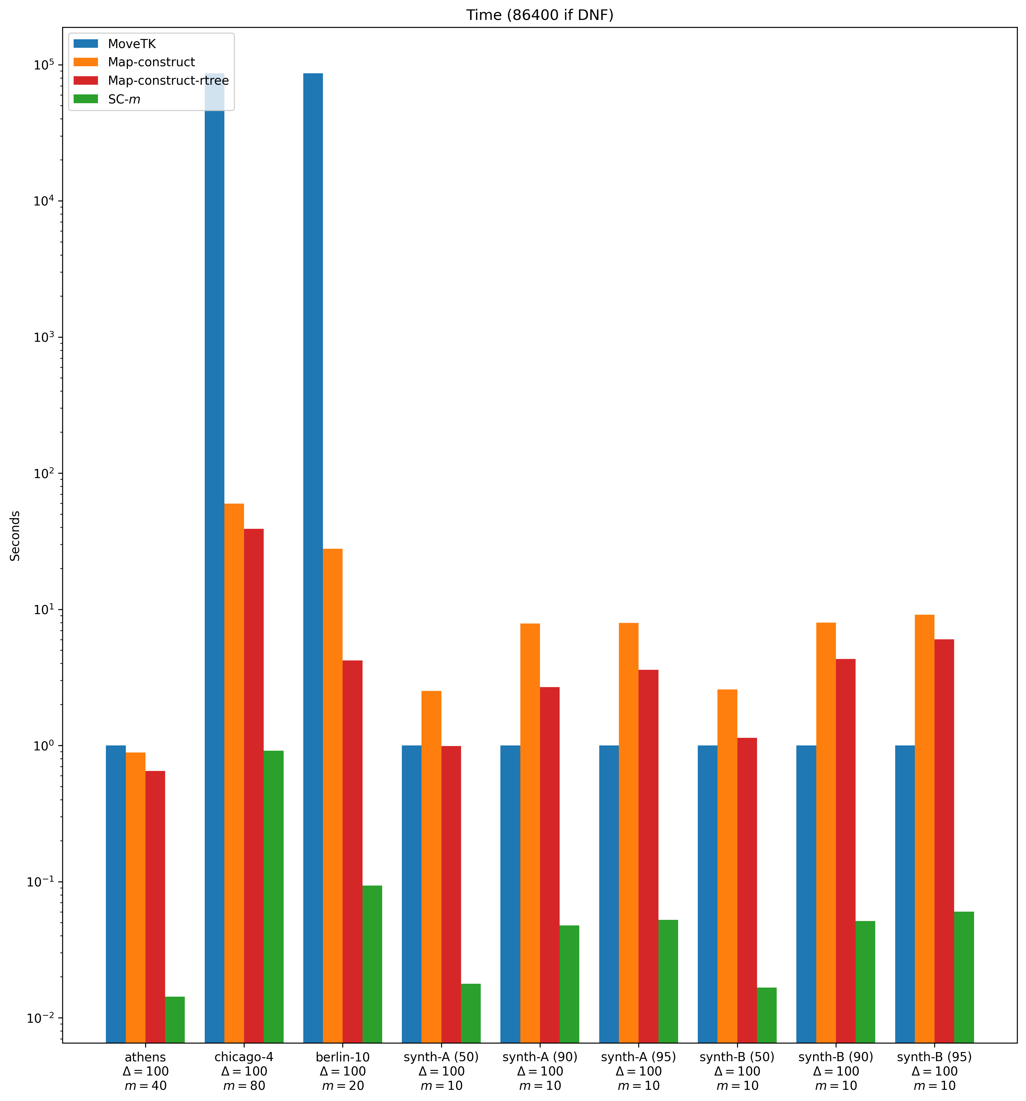
BBGLL [12] introduce the problem SC(, , , ). The input are integers , , and a set of trajectories . The goal is to find a -cluster where and . The problem statement may be altered by maximising or instead. This yields the problems SC(, , , ) and SC(, , , ). There exist three single-core implementations of these algorithms (the MOVETK library [18], map-construct [9] and map-construct-rtrees [10], a version of map-construct that uses r-trees). [18] uses space and time. Both [9, 10] use space and time, and [10] offers running time improvements over [10]. The latter uses the semi-continuous instead of discrete Fréchet distance. On the experimental input, switching between these metrics does not change the output. We do not compare to the existing GPU-based implementation [21].
Contribution.
We sketch how we optimise the BBGLL algorithm in the full version Considers two integers with (Figure 3). It alternates between StepFirst which increments , StepSecond which increments , and Query that given aims to find a -cluster with and . We apply two ideas:
- 1.
-
2.
Row generation. In [12], the StepSecond and Query functions iterate over all cells in the bottommost row of . By applying a range searching data structure, we instead only iterate over all zeroes in this row.
We note that map-construct-rtree [10] uses r-trees for row generation (we refer to the journal version [11]). However, we believe that the size of their r-tree implementation dominates the time and space used by their algorithm in our experiments. In the full version, we describe how to use a light-weight range tree to implement this principle.
Experiments.
We compare the implementations across our data sets for a variety of choices of and . We use the implementations of SC(, , , ) so that our experiments have to fix fewer parameters. Figures 4 and 5 shows the time and space usage across a subset of our experiments. The data clearly shows that our implementation is significantly more efficient than the previous single-core implementations. It is often more than a factor 1000 more efficient in terms of runtime and memory usage. We do not provide a more extensive analysis of these results since this is not our main contribution.

5 Greedy clustering using SC(, , , )
Our primary contribution is that we propose to use SC(, , , ) in a greedy clustering algorithm. On a high level, our clustering algorithm does the following:
-
We first choose the scoring function and constants (see Definition 4).
-
Our input is the set of trajectories , some , some , and an empty clustering .
-
We obtain a cluster SC(, , , ), and add it to .
-
We then remove all subtrajectories in from , and recurse.
-
We continue this process until the addition of to no longer increases .
The implementation details depend on whether we are doing -centre or -median clustering.
5.1 -centre clustering.
Given are and a set of trajectories .
We choose some integer .
The -centre clustering scoring function weighs the value: .
If is a set of -clusters (we assume there exists a cluster in whose radius is ) then:
Let be a set of -clusters and SC(, , , ). Per construction of our algorithm, and so the contribution of to Score() equals . We obtain using constant additional time throughout our algorithm. This leads to the following algorithm:
Clustering 1 ( SC-(, ) under -centre clustering).
We run Algorithm 1 for exponentially increasing where the subroutine is SC(, , , ). We then output the maximum-score clustering over all runs.
We may also fix instead of . Or, formally:
Clustering 2 ( SC-(, ) under -centre clustering ).
We run Algorithm 1 for exponentially increasing where the subroutine is SC(, , , ). We then output the maximum-score clustering over all runs.
5.2 -means clustering.
Our algorithm for -means clustering is less straightforward. To get good performance we must iterate over different choices of across the algorithm. Consider a clustering and SC(, , , ) for some . Under -centre clustering, the more points a -cluster covers, the better its scoring contribution. For -means clustering this is no longer true as the contribution of to Score() equals:
We abuse the fact that subtrajectories share no vertices to simplify the above expression to:
Consider a set of “candidate” clusters . To select the best cluster from , we use the same greedy set cover technique as [1]. We assign to every cluster a evaluation value. This is the ratio between how much it reduces the score, and how much it increases the score. I.e.,
We then select the cluster with the best evaluation among all .
Clustering 3 ( SC-(, ) under -means clustering).
We run Algorithm 2 where the subroutine is SC(, , , ).
Clustering 4 ( SC-(, ) under -means clustering ).
We run Algorithm 2 where the subroutine is SC(, , , ).
6 A new algorithm as a subroutine
Our previous clusterings 1-4 fix a parameter (or ) and subsequently only produce clusters of maximal cardinality with (or of maximum length with ).
This approach has three clear downsides:
-
1.
To find a suitable (or ) you have to train the algorithm on a smaller data set.
-
2.
Using multiple values of (or ) to broaden the search space is computationally expensive.
-
3.
Even if we fix constantly many choices for and , the corresponding algorithm has a heavily restricted solution space which affects the quality of the output.
To alleviate these downsides, we design a new algorithm based on the following observation:
Definition 5.
For fixed , we define a bivariate Boolean function where is if and only if there exists a -cluster of with and .
The functions SC(, , , ) and SC(, , , ) always output a -cluster where lies on the Pareto Front of . If clusters on the Pareto front of are good candidates to include in a clustering, then it may be worthwhile to directly compute an approximation of this Pareto front as a candidate set:
Definition 6.
Given , a set of -clusters is a -approximate Pareto front if for every -cluster there exists a with: and .
Our new algorithm, PSC(, ), iterates over a -approximate Pareto front. Storing this front explicitly uses space. Instead, we generate these clusters on the fly.
High-level description.
Let be a balanced binary tree over . Let start out as empty. Our algorithm PSC (defined by Algorithm 3) does the following:
-
For each inner node in , denote by the corresponding subtrajectory of .
-
For every prefix or suffix of , let be a -cluster maximising .
-
We add to .
Computing all prefix clusters for .
Given a trajectory and our current set , we simultaneously compute for all prefixes of a maximum-cardinality cluster and add this cluster to . We define an analogue of Definition 1:
Definition 7.
Consider row in . For let be the maximum column such that there exists a directed path from to .
Given we initialize our algorithm by storing integers and . We increment and maintain for all the value . This uses space, as does storing row . Given this data structure, we alternate between a StepSecond and Query subroutine:
StepSecond: We increment by . For each , we check if . If it is then is an isolated vertex in the graph . Thus, there exists no directed path from to any vertex in row and we set . Otherwise, which we compute in time.
Query: For a prefix of we compute a maximum-cardinality -cluster using the values (see Algorithm 4).
Note that Algorithm 4 is essentially the same as the algorithm in [12] that we described in Section 5. Thus, it computes a maximum-cardinality cluster. The key difference is that we, through , avoid walking through the free-space matrix in time to compute . We denote by Query’(, , , ) the function which computes for a suffix of a maximum-cardinality cluster in an analogous manner.
Lemma 8.
The set is a -approximate Pareto front.
Proof.
Consider any -cluster . Let . Let be the minimal subtrajectory in our tree that has as a subtrajectory. Let the children of in our tree be and . Then, by minimality of . Hence, is a suffix of , and is a prefix of . There must exist a trajectory which contains at least half as many vertices as . Since is either a prefix or suffix of a subtrajectory in our tree, we must have added some maximum-cardinality cluster to . Moreover, since is a subtrajectory of , (since any discrete walk from row to row is also a discrete walk in the Free-space matrix from row to row for ).
Theorem 9.
The algorithm PSC(, ) iterates over a -approximate Pareto front of in time using space. Here, denotes the number of zeroes in .
Proof.
Consider the balanced binary tree . Each level of depth of corresponds to a set of subtrajectories that together cover . For every such subtrajectory , both StepSecond and Query get invoked for each row . Since the tree has depth , it follows that we invoke these functions times per row of (i.e. times in total). Naively, both the StepSecond and Query functions iterate over all columns in their given row . However, just as in Section 5, we note that our functions skip over all for which . It follows that we may use our row generation trick to spend time instead ( denotes the number of zeroes in row ). Since each row gets processed times, this upper bounds our running time by .
For space, we note that invoking StepSecond and Query for a row need only rows and in memory. So the total memory usage is . Explicitly storing takes space. However, since we only iterate over , the total space usage remains . The range tree therefore dominates the space with its space usage.
6.1 Greedy clustering using PSC(, )
We reconsider Algorithms 1 and 2 in Section 5 for -centre and -means clustering. As written, these algorithms invoke a subroutine that returns a single cluster (, ). Then, the algorithm computes whether it wants to add (, ) to the current clustering. We can adapt these algorithms to this new function. For , we invoke PSC(, ). This function iterates over a set of clusters (, ). For each cluster (, ) that we encounter, we let either Algorithm 1 or 2 compute whether it wants to add (, ) to the current clustering.
7 Experiments
We propose three new greedy clustering algorithms for -centre clustering:
-
1.
SC- runs Algorithm 1, for exponentially scaling , with SC(, , , ),
-
2.
SC- runs Algorithm 1, for exponentially scaling , with SC(, , , ), and
-
3.
PSC runs Algorithm 1, for exponentially scaling , with ).
Our algorithms SC- and SC- need to fix a parameter and respectively. We choose and and do a separate run for each choice. Thus, together with PSC, we run ten different algorithm configurations. We additionally compare to the subtrajectory clustering algorithm from [10], which is oblivious to the scoring function.
-
Map-construction runs the algorithm in [10]. We terminate this map construction algorithm as soon as it has constructed a clustering of .
-means clustering.
For -means clustering, we obtain three algorithms by running Algorithm 2 instead. Note that our clustering algorithms invoked Algorithm 1 across several runs for exponentially scaling . Our clustering algorithms do not invoke Algorithm 2 in this manner. Instead, Algorithm 2 considers exponentially scaling ’s internally. Our experiments show that this heavily impacts the clustering’s performance on large input.
We again obtain ten algorithm configurations. In addition, we run the map construction algorithm from [10] and the -means subtrajectory clustering algorithms from [1]:
-
Envelope runs the algorithm from [1] with the scoring parameters .
Experimental setup.
We design different experiments to measure performance and the scoring function. For performance, we run fourteen experiments across the five real-world data sets. Seven experiments for -centre clustering, and seven for -means clustering. Each experiment ran three times, using a different vector . Each experiment runs programs for -centre clustering, or for -means clustering. If a program fails to terminate after 24 hours, we do not extract any output or memory usage.
We restrict scoring measurements to the three smaller or subsampled real-world data sets. This is necessary to make Map-construct and Envelope terminate. We add six synthetic data sets. We only compare under -means clustering since only our algorithms can optimise for -centre clustering. The experiments were conducted on a machine with a 4.2GHz AMD Ryzen 9 7950X3D and 128GB memory. Over 90 runs hit the timeout. Running the total set of experiments sequentially takes over 100 days on this machine.
The full results per experiment are organised in tables in the full version. Here, we restrict our attention to only three plots.
Choosing .
Recall that weighs the number of clusters in the clustering and that weighs the fraction of uncovered points. We follow the precedent set in [1] and choose , and equal to the number of trajectories in . Finally, weighs the Fréchet distance across clusters. For each data set, we first find a choice for such the algorithms lead to a non-trivial clustering. We then also run the algorithms using the scoring vectors and , for a total of three scoring vectors per data set.
Comparing quality.
To compare solution quality, we measure the scoring function and other qualities such as: the total number of clusters in the clustering, the maximum Fréchet distance from a subtrajectory to its centre, and the average Fréchet distance across clusters. Our competitor algorithms frequently time out on the real-world data sets. Hence, the qualitative comparison also makes use of our synthetic data set. We use three different configurations of our synthetic set to create input of different size. We choose to compare only under -means clustering for a more fair comparison to other algorithms. Indeed, the algorithm by [1] was designed for the -means metric ([10] is scoring function oblivious). Consequently, comparing under -centre would only give us an unfair advantage.
7.1 Results for -means clustering
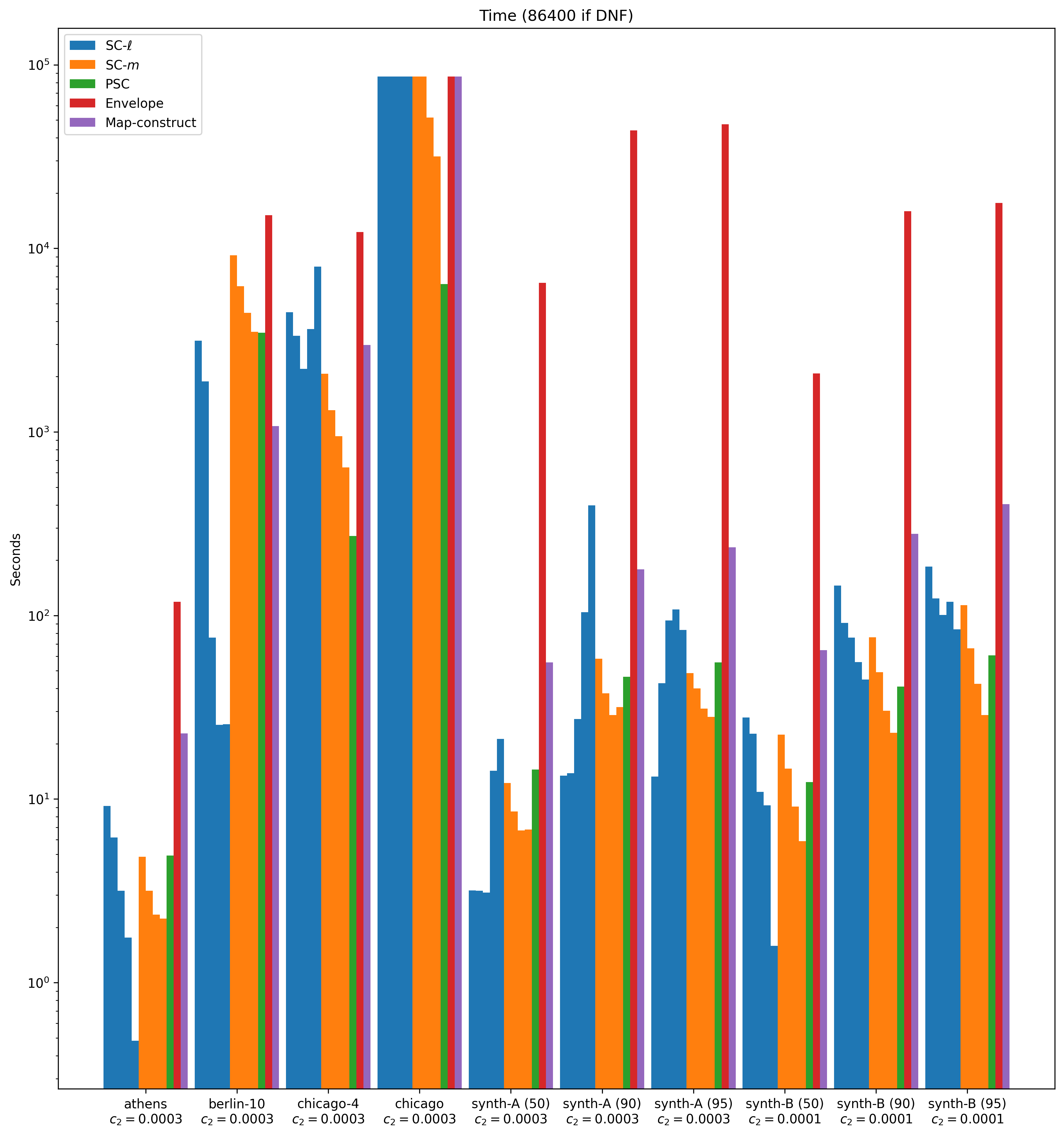
The bar plot in Figure 6 visualizes how the algorithms score. Figures 7 and 8 show, respectively, a logarithmic-scale plot of the time and space usage. These plots use the “medium” choice for for each data set. Note that our choice of is very similar across the data sets in the figure. This is because Athens, Berlin and Chicago come from the same source, and thereby have the same scaling. We subsequently designed our synthetic data to match this scaling. Plots for the other scoring vector choices are contained in the full version.
Clustering quality.
Figure 6 shows that Map-construct (which is oblivious to the scoring function) scores poorly on all inputs. One reasons for this is that it always outputs a large number of clusters. The Envelope algorithm, which was specifically designed for this scoring function, almost always obtains the best score.
For any data set, for any scoring vector, we always find a choice for (or ) where SC- and SC- obtain a comparable score to Envelope. The algorithm PSC scores best out of all newly proposed clustering algorithms. Across all data sets and scoring functions it frequently competes with, and sometimes even improves upon, the score of Envelope.

Other quality metrics.
We briefly note that the full data in the appendix also considers other quality metrics: the number of clusters and the maximum and average Fréchet distance within a cluster. Perhaps surprisingly, Map-construct does not perform better on the latter two metrics even though it outputs many clusters. Envelope scores worse on these metrics across nearly all data sets and scoring vectors. However, it stays within a competitive range.
Runtime comparison.
Figure 7 shows the runtime performance in logarithmic scale. On the Berlin data set, no algorithm terminates in time. On Drifter and UniD, only PSC terminates within the time limit. In the figure, we consider the synthetic data sets their place.
Envelope may produce high-quality clusterings, but takes significant time to do so. Despite using considerably less memory than Map-construct, it is consistently more than a factor two slower. Our algorithms SC- and SC- can always find a choice of or such that previous algorithms are orders of magnitude slower. Our PSC algorithm is always orders of magnitude faster than the existing clustering algorithms. This is especially true on larger data sets, which illustrates that our algorithms have better scaling.
When we compare our own algorithms, we note that we can frequently find a choice for such that SC- is significantly faster than SC- and PSC. However, when considering the runtime to quality ratio, PSC appears to be a clear winner.
Memory consumption.
Figure 8 shows memory performance on a logarithmic scale. The figure excludes Drifter, UniD and Berlin for the same reason as when comparing running times. We record zero memory usage whenever an algorithm times out.
We observe that Map-construct uses an order of magnitude more memory than its competitors. This is because it stores up to candidate clusters in memory, together with the entire free-space matrix for various choices of . Envelope also has a large memory footprint and uses at least a factor more memory on all of the inputs.
When comparing our own implementations, we observe that SC- and PSC have a very small memory footprint. These algorithms use and space. Since we fix to be a small constant, both algorithms use near linear space. The space usage of SC- is where is the length of the longest subtrajectory such that there exists a -cluster with . The data shows that for many choices of , this space is considerable. Yet, it is still considerably lower than pre-existing algorithms.
7.2 Results for -centre clustering
When comparing score, runtime, or memory usage under -centre clustering, we reach the same conclusions. The only difference is that the performance of SC- becomes more competitive to SC- and PSC on large data sets. This is because SC(, , , uses much time and space whenever both the data set and are large. Our -means clustering meta-algorithm considers a large each round, and invokes SC(, , , every round.
Our -centre clustering meta-algorithm has a separate run for each . If is large, it terminates quickly because it adds very high-cardinality clusters to the clustering. This speeds up all our implementations, but SC- the most.
8 Conclusion
We proposed new subtrajectory clustering algorithms. Our first two approaches use the algorithms SC(, , , ) and SC(, , , ) by BBGLL [12]. We use these algorithms as a subroutine in a greedy clustering algorithm to cluster a set of trajectories .
Consider the Boolean function that outputs true if there exists a -cluster of with and . We observe that these functions always output a point on the Pareto front of this function. We show a new algorithm PSC(, ) that, instead of returning a single cluster on this Pareto front, iterates over a -approximation of this Pareto front instead. Intuitively, this function iterates over a broader set of candidate clusters that have comparable quality to any output of SC(, , , ) and SC(, , , ). We create a greedy clustering algorithm PSC using this algorithm as a subroutine.
Our analysis shows that our new clustering algorithms significantly outperform previous algorithms in running time and space usage. We primarily use the scoring function from [1] to measure clustering quality and observe that our algorithms give competitive scores. For other quality metrics, our algorithms often perform better than their competitors. We observe that PSC is the best algorithm when comparing the ratio between score and performance.
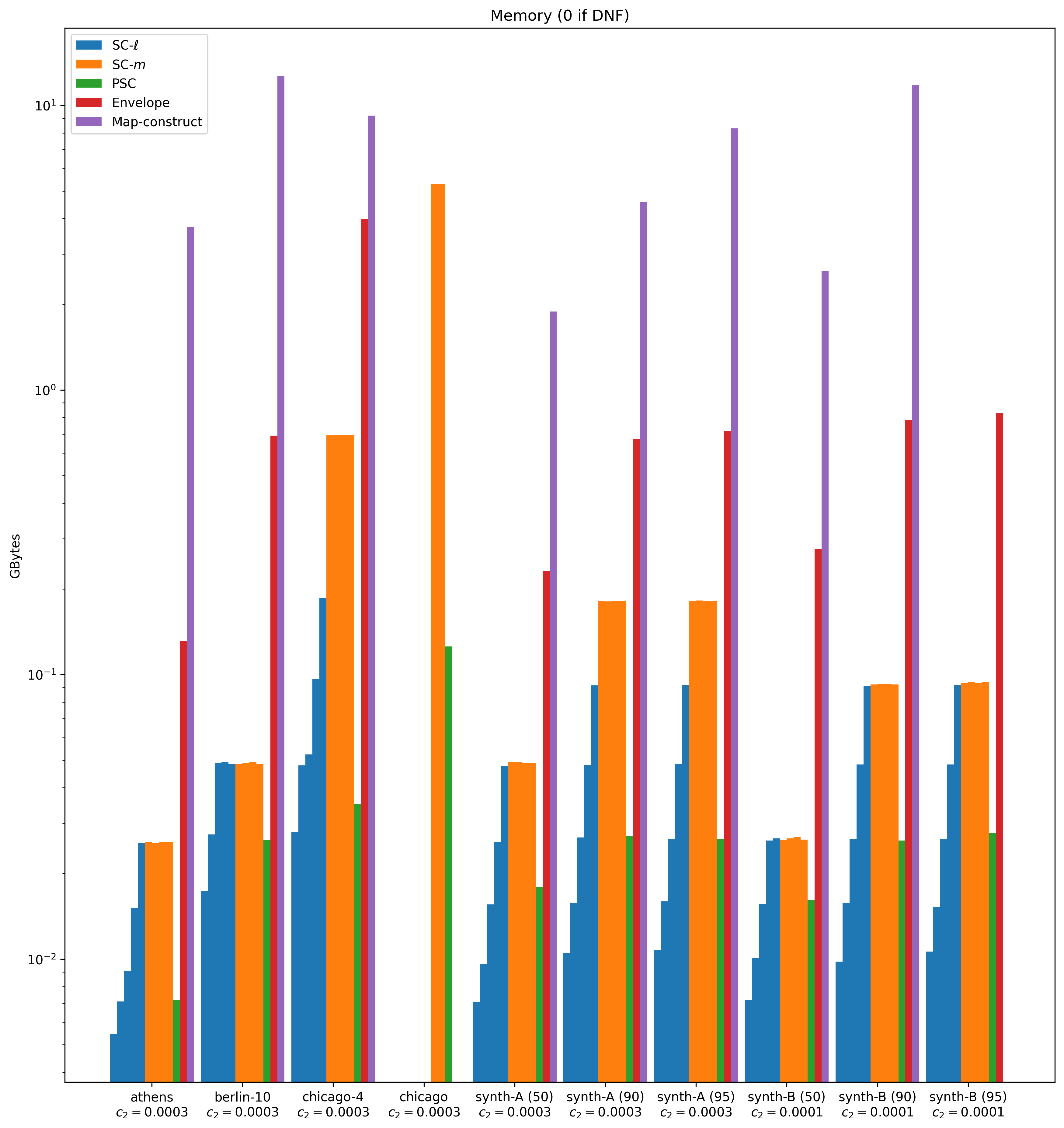
Whenever a run did not terminate, we display a memory usage of zero.
References
- [1] Pankaj K Agarwal, Kyle Fox, Kamesh Munagala, Abhinandan Nath, Jiangwei Pan, and Erin Taylor. Subtrajectory clustering: Models and algorithms. ACM SIGMOD-SIGACT-SIGAI Symposium on Principles of Database Systems (PODS), pages 75–87, 2018. doi:10.1145/3196959.3196972.
- [2] Mahmuda Ahmed, Sophia Karagiorgou, Dieter Pfoser, and Carola Wenk. A comparison and evaluation of map construction algorithms using vehicle tracking data. GeoInformatica, 19:601–632, 2015. doi:10.1007/s10707-014-0222-6.
- [3] Mahmuda Ahmed and Carola Wenk. Constructing street networks from gps trajectories. European Symposium on Algorithms (ESA), pages 60–71, 2012. doi:10.1007/978-3-642-33090-2_7.
- [4] Hugo Akitaya, Frederik Brüning, Erin Chambers, and Anne Driemel. Subtrajectory Clustering: Finding Set Covers for Set Systems of Subcurves. Computing in Geometry and Topology, 2(1):1:1–1:48, 2023. doi:10.57717/cgt.v2i1.7.
- [5] Helmut Alt and Michael Godau. Computing the fréchet distance between two polygonal curves. International Journal of Computational Geometry & Applications, 5:75–91, 1995. doi:10.1142/S0218195995000064.
- [6] James Biagioni and Jakob Eriksson. Map inference in the face of noise and disparity. ACM International Conference on Advances in Geographic Information Systems (SIGSPATIAL), pages 79–88, 2012. doi:10.1145/2424321.2424333.
- [7] Jiang Bian, Dayong Tian, Yuanyan Tang, and Dacheng Tao. A survey on trajectory clustering analysis. arXiv preprint arXiv:1802.06971, 2018. arXiv:1802.06971.
- [8] Frederik Brüning, Jacobus Conradi, and Anne Driemel. Faster Approximate Covering of Subcurves Under the Fréchet Distance. In Shiri Chechik, Gonzalo Navarro, Eva Rotenberg, and Grzegorz Herman, editors, European Symposium on Algorithms (ESA 2022), volume 244 of Leibniz International Proceedings in Informatics (LIPIcs), pages 28:1–28:16, Dagstuhl, Germany, 2022. Schloss Dagstuhl – Leibniz-Zentrum für Informatik. doi:10.4230/LIPIcs.ESA.2022.28.
- [9] Kevin Buchin, Maike Buchin, David Duran, Brittany Terese Fasy, Roel Jacobs, Vera Sacristan, Rodrigo I Silveira, Frank Staals, and Carola Wenk. Clustering trajectories for map construction. ACM International Conference on Advances in Geographic Information Systems (SIGSPATIAL), pages 1–10, 2017. doi:10.1145/3139958.3139964.
- [10] Kevin Buchin, Maike Buchin, Joachim Gudmundsson, Jorren Hendriks, Erfan Hosseini Sereshgi, Vera Sacristán, Rodrigo I Silveira, Jorrick Sleijster, Frank Staals, and Carola Wenk. Improved map construction using subtrajectory clustering. ACM Workshop on Location-Based Recommendations, Geosocial Networks, and Geoadvertising (SIGSPATIAL), pages 1–4, 2020. doi:10.1145/3423334.3431451.
- [11] Kevin Buchin, Maike Buchin, Joachim Gudmundsson, Jorren Hendriks, Erfan Hosseini Sereshgi, Rodrigo I Silveira, Jorrick Sleijster, Frank Staals, and Carola Wenk. Roadster: Improved algorithms for subtrajectory clustering and map construction. Computers & Geosciences, 196:105845, 2025. doi:10.1016/j.cageo.2024.105845.
- [12] Kevin Buchin, Maike Buchin, Joachim Gudmundsson, Maarten Löffler, and Jun Luo. Detecting commuting patterns by clustering subtrajectories. International Journal of Computational Geometry & Applications, 21(03):253–282, 2011. doi:10.1142/S0218195911003638.
- [13] Kevin Buchin, Maike Buchin, Marc Van Kreveld, Maarten Löffler, Rodrigo I Silveira, Carola Wenk, and Lionov Wiratma. Median trajectories. Algorithmica, 66:595–614, 2013. doi:10.1007/s00453-012-9654-2.
- [14] Lili Cao and John Krumm. From gps traces to a routable road map. ACM international conference on advances in geographic information systems (SIGSPATIAL), pages 3–12, 2009. doi:10.1145/1653771.1653776.
- [15] Chen Chen, Hao Su, Qixing Huang, Lin Zhang, and Leonidas Guibas. Pathlet learning for compressing and planning trajectories. ACM International Conference on Advances in Geographic Information Systems (SIGSPATIAL), pages 392–395, 2013. doi:10.1145/2525314.2525443.
- [16] Jacobus Conradi and Anne Driemel. Finding complex patterns in trajectory data via geometric set cover. arXiv preprint arXiv:2308.14865, 2023. doi:10.48550/arXiv.2308.14865.
- [17] Jonathan J Davies, Alastair R Beresford, and Andy Hopper. Scalable, distributed, real-time map generation. IEEE Pervasive Computing, 5(4):47–54, 2006. doi:10.1109/MPRV.2006.83.
- [18] university of Technology Eindhoven. MoveTK: the movement toolkit. http://https://github.com/movetk/movetk, 2020.
- [19] Scott Gaffney and Padhraic Smyth. Trajectory clustering with mixtures of regression models. ACM International Conference on Knowledge Discovery and Data mining (SIGKDD), pages 63–72, 1999. doi:10.1145/312129.312197.
- [20] Joachim Gudmundsson, Andreas Thom, and Jan Vahrenhold. Of motifs and goals: mining trajectory data. ACM International Conference on Advances in Geographic Information Systems (SIGSPATIAL), pages 129–138, 2012. doi:10.1145/2424321.2424339.
- [21] Joachim Gudmundsson and Nacho Valladares. A GPU approach to subtrajectory clustering using the fréchet distance. ACM nternational Conference on Advances in Geographic Information Systems (SIGSPATIAL), pages 259–268, 2012. doi:10.1145/2424321.2424355.
- [22] Joachim Gudmundsson and Sampson Wong. Cubic upper and lower bounds for subtrajectory clustering under the continuous fréchet distance. ACM-SIAM Symposium on Discrete Algorithms (SODA), pages 173–189, 2022. doi:10.1137/1.9781611977073.9.
- [23] Jincai Huang, Min Deng, Jianbo Tang, Shuling Hu, Huimin Liu, Sembeto Wariyo, and Jinqiang He. Automatic generation of road maps from low quality gps trajectory data via structure learning. IEEE Access, 6:71965–71975, 2018. doi:10.1109/ACCESS.2018.2882581.
- [24] Chih-Chieh Hung, Wen-Chih Peng, and Wang-Chien Lee. Clustering and aggregating clues of trajectories for mining trajectory patterns and routes. The VLDB Journal, 24:169–192, 2015. doi:10.1007/s00778-011-0262-6.
- [25] Sophia Karagiorgou and Dieter Pfoser. On vehicle tracking data-based road network generation. ACM International Conference on Advances in Geographic Information Systems (SIGSPATIAL), pages 89–98, 2012. doi:10.1145/2424321.2424334.
- [26] Sophia Karagiorgou, Dieter Pfoser, and Dimitrios Skoutas. Segmentation-based road network construction. ACM International Conference on Advances in Geographic Information Systems (SIGSPATIAL), pages 460–463, 2013. doi:10.1145/2525314.2525460.
- [27] Jae-Gil Lee, Jiawei Han, and Kyu-Young Whang. Trajectory clustering: a partition-and-group framework. ACM International Conference on Management of Data (SIGMOD), pages 593–604, 2007. doi:10.1145/1247480.1247546.
- [28] Vanessa Lago Machado, Ronaldo dos Santos Mello, Vânia Bogorny, and Geomar André Schreiner. A survey on the computation of representative trajectories. GeoInformatica, pages 1–26, 2024. doi:10.1007/s10707-024-00514-y.
- [29] Tobias Moers, Lennart Vater, Robert Krajewski, Julian Bock, Adrian Zlocki, and Lutz Eckstein. The exid dataset: A real-world trajectory dataset of highly interactive highway scenarios in germany. 2022 IEEE Intelligent Vehicles Symposium (IV), pages 958–964, 2022. doi:10.1109/IV51971.2022.9827305.
- [30] Cynthia Sung, Dan Feldman, and Daniela Rus. Trajectory clustering for motion prediction. IEEE/RSJ International Conference on Intelligent Robots and Systems (IROS), pages 1547–1552, 2012. doi:10.1109/IROS.2012.6386017.
- [31] Suyi Wang, Yusu Wang, and Yanjie Li. Efficient map reconstruction and augmentation via topological methods. ACM International Conference on Advances in Geographic Information Systems (SIGSPATIAL), pages 1–10, 2015. doi:10.1145/2820783.2820833.