Efficient Neural Network Verification via Order Leading Exploration of Branch-and-Bound Trees

Essentially, our proposed approach changes the naive “breadth-first” exploration of the sub-problem space in the classic $\mathrm{𝙱𝚊𝙱}$ to an intelligent way guided by the likelihood of finding counterexamples in different sub-problems. However, as this guidance consists of a total order over different branches, it may lose some chances of finding counterexamples in some branches that initially seem not promising.

To mitigate this issue, we also propose a variant of our approach, inspired by simulated annealing [24]. It works as follows: throughout the process, we maintain a temperature that keeps decreasing slowly, which is used to control the trade-off between “exploitation” and “exploration”. Initially, when the temperature is high, our algorithm tends to explore the sub-problem space by assigning a considerably high probability to accept a sub-problem that is not promising; as temperature goes down, it converges to the optimal sub-problem; due to the exploration of the search space at the initial stage, the algorithm is likely to converge to the globally optimal sub-problems. In this way, we can mitigate the side-effect of being too greedy, and strike a balance between “exploitation” and “exploration”.

Approximated verifiers, denoted as $\mathrm{𝙻𝚙𝚅𝚎𝚛𝚒𝚏𝚒𝚎𝚛}$, are a class of verifiers that solve a verification problem by computing an over-approximation of the output region of neural networks – if the over-approximation satisfies the specification, it implies that the original output region must also satisfy it. Typically, $\mathrm{𝙻𝚙𝚅𝚎𝚛𝚒𝚏𝚒𝚎𝚛}$ can return a tuple $⟨\widehat{p},\widehat{𝒙}⟩$, where $\widehat{p}\in ℝ$ is called a verifier assessment, which is a quantity that indicates the extent to which the over-approximated output satisfies the specification. Formally, given an $\mathrm{𝙻𝚙𝚅𝚎𝚛𝚒𝚏𝚒𝚎𝚛}$, it can construct a region $\widehat{\mathrm{\Omega }}\supseteq \{N(𝒙)\mid \mathrm{\Phi }(𝒙)=\mathrm{𝗍𝗋𝗎𝖾}\}$, which over-approximates the output region of a neural network $N$; then, $\mathrm{𝙻𝚙𝚅𝚎𝚛𝚒𝚏𝚒𝚎𝚛}$ computes $\widehat{p}$ as follows: $\widehat{p}:={\min }_{𝒚\in \widehat{\mathrm{\Omega }}}f(𝒚)$, where $f$ is as defined in Def. 2. If $\widehat{p}$ is positive, it implies that the original output also satisfies the specification, and so it can certify the satisfaction of neural networks. Conversely, if $\widehat{p}$ is negative, $\mathrm{𝙻𝚙𝚅𝚎𝚛𝚒𝚏𝚒𝚎𝚛}$ deems that the specification is violated and provides a counterexample input $\widehat{𝒙}$ as an evidence. However, due to the over-approximation, this reported violation of $\mathrm{𝙻𝚙𝚅𝚎𝚛𝚒𝚏𝚒𝚎𝚛}$ could be a false alarm and the counterexample $\widehat{𝒙}$ may be a spurious one, i.e., the corresponding output $N(\widehat{𝒙})$ of $\widehat{𝒙}$ actually satisfies the specification. In this case, just based on the result of $\mathrm{𝙻𝚙𝚅𝚎𝚛𝚒𝚏𝚒𝚎𝚛}$, we cannot infer whether $N$ holds or violates the specification. This situation is referred to as the completeness issue of approximated verifiers.

There have been various approximation strategies that can be used to implement approximated verifiers, e.g., DeepPoly [44] and ReluVal [50], and mostly, the over-approximation is accomplished by using linear constraints to bound the output range of the non-linear ReLU functions. In particular, we assume that our adopted approximated verifiers hold the monotonicity property, namely, for two output regions of neural networks that hold ${\mathrm{\Omega }}_1\subset {\mathrm{\Omega }}_2$, if we over-approximate them by using the same approximated verifier $\mathrm{𝙻𝚙𝚅𝚎𝚛𝚒𝚏𝚒𝚎𝚛}$, the obtained over-approximation ${\widehat{\mathrm{\Omega }}}_1$ and ${\widehat{\mathrm{\Omega }}}_2$ hold that ${\widehat{\mathrm{\Omega }}}_1\subseteq {\widehat{\mathrm{\Omega }}}_2$. While there can be different options of over-approximation strategies, our proposed approach is orthogonal to them, so we can adopt any approximated verifiers that hold our assumption about monotonicity.

$\mathrm{𝙱𝚊𝙱}$ is the state-of-the-art neural network verification approach, and has been adopted in several advanced verification tools, such as $\alpha \beta$-Crown [51] and Marabou [52]. It is essentially a “divide-and-conquer” strategy, that divides a verification problem adaptively and applies off-the-shelf verifiers (such as approximated verifiers) to solve the sub-problems. Because approximated verifiers often achieve better precision on sub-problems, $\mathrm{𝙱𝚊𝙱}$ can thus overcome the weaknesses of the plain application of approximated verifiers to the original problem and resolve the issues of false alarms.

Before looking into the details of $\mathrm{𝙱𝚊𝙱}$, we first introduce ReLU specification, which is an important notion in the algorithm of $\mathrm{𝙱𝚊𝙱}$.

By selecting a neuron $i$, we can split the ReLU function into two linear functions, each identified by a predicate $r_i^{+}$ or $r_i^{-}$ over the input of ReLU. Thereby, a neural network verification problem boils down to two sub-problems, for each of which $\mathrm{𝙻𝚙𝚅𝚎𝚛𝚒𝚏𝚒𝚎𝚛}$ does not need to perform over-approximation for the ReLU function in the $i$-th neuron.

The workflow of $\mathrm{𝙱𝚊𝙱}$ is presented in Alg. 1. In Alg. 1, we allow $\mathrm{𝙻𝚙𝚅𝚎𝚛𝚒𝚏𝚒𝚎𝚛}$ to take an additional argument, namely, a ReLU specification $\mathrm{\Gamma }$, which identifies a sub-problem by adding the constraints in $\mathrm{𝖲𝖾𝗍}(\mathrm{\Gamma })$ to constrain the inputs of a number of selected ReLU functions. It uses a FIFO queue $Q$ to maintain the problem to be solved, which is initialized to be a set that consists of $\top$ only, identifying the original verification problem.

1. i)

   First, it applies $\mathrm{𝙻𝚙𝚅𝚎𝚛𝚒𝚏𝚒𝚎𝚛}$ to the original problem (Line 7): if $\mathrm{𝙻𝚙𝚅𝚎𝚛𝚒𝚏𝚒𝚎𝚛}$ returns a positive $\widehat{p}$, or a negative $\widehat{p}$ with a valid counterexample $\widehat{𝒙}$ (Line 10), then verification can be terminated with a verdict returned accordingly;

2. ii)

   In the case it returns a negative $\widehat{p}$ with a spurious counterexample (Line 12), it divides the verification problem into two sub-problems. This is achieved by first selecting a neuron (i.e., a ReLU) in the network according to a pre-defined ReLU selection heuristics $𝖧$ (Line 13), and then identifying two sub-problems each identified by an additional constraint on the input of the selected ReLU function (Line 15).

3. iii)

   It applies $\mathrm{𝙻𝚙𝚅𝚎𝚛𝚒𝚏𝚒𝚎𝚛}$ to the new sub-problems respectively, and decides whether it needs to further split the sub-problem, following the same rule in Step ii. In Alg. 1, this is implemented by recursive call of the BaB function in Line 16.

In $\mathrm{𝙱𝚊𝙱}$, the ReLU selection heuristics $𝖧$ involves an order over different neurons such that it can select the next ReLU based on an existing ReLU specification. There has been a rich body of literature that proposes different ReLU selection strategies, such as DeepSplit [21] and FSB [10]. However, our proposed approach in §4 is orthogonal to these strategies and so it can work with existing strategies. In this work, we follow an existing neural network verification approach [48] and we adopt the state-of-the-art ReLU selection strategy in [21].

As a result of Alg. 1, it forms a binary tree $𝒯$ (see Line 2 and Line 8) that records the history of problem splitting during the $\mathrm{𝙱𝚊𝙱}$ process. In this tree, each node $⟨\mathrm{\Gamma },\widehat{p}⟩$ denotes a sub-problem, identified by a ReLU specification $\mathrm{\Gamma }$ and the verifier assessment $\widehat{p}$ returned by $\mathrm{𝙻𝚙𝚅𝚎𝚛𝚒𝚏𝚒𝚎𝚛}$ that signifies the satisfaction of the sub-problem.

The main loop in Line 5 of Alg. 2 can be terminated on the satisfaction of any of the following three conditions:

• $\mathrm{■}$

  $𝖱(\epsilon )=-\mathrm{\infty }$: This implies that all leaf nodes have been verified successfully (i.e., $\widehat{p}>0$ for all leaves, otherwise by Line 20 $𝖱(\epsilon )$ cannot be $-\mathrm{\infty }$), allowing the algorithm to return a $\mathrm{𝗍𝗋𝗎𝖾}$ verdict that certifies the specification satisfaction;

• $\mathrm{■}$

  $𝖱(\epsilon )=+\mathrm{\infty }$: This implies that a valid counterexample has been found in some leaf node, and so by Line 20 its suspiciousness of $+\mathrm{\infty }$ can be back-propagated to the root node; in this case, the algorithm can be terminated with a $\mathrm{𝖿𝖺𝗅𝗌𝖾}$ verdict;

• $\mathrm{■}$

  $\mathrm{𝚝𝚒𝚖𝚎𝚘𝚞𝚝}$: This occurs when the algorithm exceeds its allocated time budget without reaching either of the above conclusive verdicts.

The three termination conditions correspond to the three cases of return in Line 7.

Hill climbing is a stochastic optimization technique that aims to find the optimum of a black-box function. Due to the black-box nature of the objective function, it relies on sampling in the search space and selects only the samples that optimize the objective function as the direction to move. Therefore, this is a greedy strategy, similarly to our proposed approach ${\mathrm{𝖮𝗅𝗂𝗏𝖺}}^{\mathrm{𝖦𝖱}}$ in §4.2. While ${\mathrm{𝖮𝗅𝗂𝗏𝖺}}^{\mathrm{𝖦𝖱}}$ does not need to sample the search space, it can select the sub-problem that is more promising, and thereby move towards the direction that is more likely to achieve the objective. As a consequence, they both suffer from the issue of “local optima”.

In the field of stochastic optimization, simulated annealing [24] is an effective approach to mitigate the issue of “local optima” in hill climbing. It is inspired by the process of annealing in metallurgy, in which the temperature is initially high but slowly decreases such that the physical properties of metals can be stabilized. In simulated annealing, there is also a temperature that slowly decreases throughout the process: when the temperature is initially high, it tends to explore the search space and assigns a considerably high probability to accept a sample that is not the optimal; as temperature goes down, it converges to the optimum that is likely to be the global one, thanks to the exploration of the search space at the initial stage.

Our proposed approach ${\mathrm{𝖮𝗅𝗂𝗏𝖺}}^{\mathrm{𝖲𝖠}}$ adapts simulated annealing to our problem setting, and the core idea involves that, at the initial stage, we allow more chances of exploring the branches that are less promising. Then, after we have comprehensively explored the search space and obtained the information about the suspiciousness of different branches, we tend to exploit the branches that are more suspicious, namely, that are more likely to contain counterexamples.

The ${\mathrm{𝖮𝗅𝗂𝗏𝖺}}^{\mathrm{𝖲𝖠}}$ algorithm is presented in Alg. 3. It also starts with checking the original verification problem (Line 2), and enters the loop of tree exploration if the original problem cannot be solved by $\mathrm{𝙻𝚙𝚅𝚎𝚛𝚒𝚏𝚒𝚎𝚛}$ (Line 5). However, compared to ${\mathrm{𝖮𝗅𝗂𝗏𝖺}}^{\mathrm{𝖲𝖠}}$, it has a notable difference about the adoption of a temperature $T$ (Line 4) which is a global variable that keeps decreasing in each loop of the algorithm (Line 7).

In the function SABaB, the temperature $T$ is used when selecting the nodes to proceed. In the case if the children of the current node $\mathrm{\Gamma }$ have been expanded (Line 14), unlike ${\mathrm{𝖮𝗅𝗂𝗏𝖺}}^{\mathrm{𝖦𝖱}}$ that always prefers the most suspicious child, ${\mathrm{𝖮𝗅𝗂𝗏𝖺}}^{\mathrm{𝖲𝖠}}$ selects a child according to the policy adapted from the original simulated annealing:

• $\mathrm{■}$

  It first computes an acceptance probability $\mathrm{\Delta }p$ (Line 15), by which it determines whether the selection of a child that is less promising is acceptable. This probability $\mathrm{\Delta }p$ is decided by both the difference of “energy” (defined by the suspiciousness difference between two children) and the temperature $T$;

• $\mathrm{■}$

  In the original simulated annealing, a sample that is more promising can be accepted in any case, and a sample that is less promising can be accepted with the probability $\mathrm{\Delta }p$. In our context, we adapt this policy as follows (Line 16):

  • –

    If a random value in $[0,1]$ is less than $\mathrm{\Delta }p$, we randomly select a child from the two children of $\mathrm{\Gamma }$ with the same probability, despite the CePO order over the two children;

  • –

    Otherwise, we select the more suspicious child following the CePO order.

The selected child will be used as the argument for the recursive call of SABaB, in order to proceed towards a node whose children are not expanded. After achieving such a node $\mathrm{\Gamma }$, it expands the children of $\mathrm{\Gamma }$ (Lines 19-22) by applying $\mathrm{𝙻𝚙𝚅𝚎𝚛𝚒𝚏𝚒𝚎𝚛}$ to each child of $\mathrm{\Gamma }$, recording their suspiciousness (Line 21) and updating the $\mathrm{𝙱𝚊𝙱}$ tree (Line 22). Lastly, it back-propagates the greater suspiciousness over the children until the root (Line 23), similarly to ${\mathrm{𝖮𝗅𝗂𝗏𝖺}}^{\mathrm{𝖲𝖠}}$.

This gradual transition from exploration to exploitation helps ${\mathrm{𝖮𝗅𝗂𝗏𝖺}}^{\mathrm{𝖲𝖠}}$ to avoid premature convergence while ensuring an eventual focus on the promising branches. The termination conditions remain the same as in ${\mathrm{𝖮𝗅𝗂𝗏𝖺}}^{\mathrm{𝖦𝖱}}$, checking for full verification ($𝖱(\epsilon )=-\mathrm{\infty }$), counterexample discovery ($𝖱(\epsilon )=+\mathrm{\infty }$), or timeout. However, by pursuing a higher coverage of the sub-problem space before being greedy, ${\mathrm{𝖮𝗅𝗂𝗏𝖺}}^{\mathrm{𝖲𝖠}}$ increases the possibility of discovering counterexamples that might be missed by the purely greedy strategy of ${\mathrm{𝖮𝗅𝗂𝗏𝖺}}^{\mathrm{𝖦𝖱}}$.

We compare the two versions of $\mathrm{𝖮𝗅𝗂𝗏𝖺}$, namely, ${\mathrm{𝖮𝗅𝗂𝗏𝖺}}^{\mathrm{𝖦𝖱}}$ and ${\mathrm{𝖮𝗅𝗂𝗏𝖺}}^{\mathrm{𝖲𝖠}}$, with three state-of-the-art neural network verification tools $\alpha \beta$-Crown [59, 51], NeuralSAT [11], and $\mathrm{𝙱𝚊𝙱}$-baseline, as presented in §3.2. The settings of baseline approaches are detailed below:

• $\mathrm{■}$

  $\mathrm{𝙱𝚊𝙱}$-baseline is implemented based on the ERAN framework [41, 44], which employs LP-based triangle relaxation for bounding the output of ReLU functions, and utilizes DeepSplit [21] as the ReLU selection heuristics for selecting ReLU function to split, i.e., $𝖧$ in Alg. 1, Alg. 2, and Alg. 3.

• $\mathrm{■}$

  $\alpha \beta$-Crown [59, 51] is applied with its default branch-and-bound settings. Moreover, a balanced strategy kFSB from FSB [10] is selected as the ReLU selection heuristics for selecting the ReLU function to split.

• $\mathrm{■}$

  NeuralSAT [11] is applied with its default DPLL(T) framework and we select the stabilized optimization as the neuron stability heuristics for ReLU activation pattern search. Additionally, it is registered with a random attack [8, 56] to reject the easily detected violation instances at the early stage of verification processes.

For our approaches, the hyperparameters are set as follows: $\lambda =0.5$ (see Def. 6), $T_{max}=1$ (see Line 4 of Alg. 3) and $\alpha =0.99$ (see Line 7 of Alg. 3); in RQ3, we study the impact of these hyperparameters on the performance of our approaches.

We apply each of the five approaches (including two proposed approaches and three baseline approaches) to each of the verification problems, and we adopt 1000 secs as our time budget, following the VNN-COMP competition [30]. If an approach manages to solve the problem (either verifies the problem or reports a real counterexample), we deem this run as a solved verification process, and record the time cost for reaching the verification conclusion. In particular, our ${\mathrm{𝖮𝗅𝗂𝗏𝖺}}^{\mathrm{𝖲𝖠}}$ is a stochastic approach, namely, its performance is subject to randomness. To compare its performance with other approaches, in Table 2, Table 3 and Fig. 5, we only show the performance of one random run; in Fig. 6, we particularly study the influence of randomness to ${\mathrm{𝖮𝗅𝗂𝗏𝖺}}^{\mathrm{𝖲𝖠}}$, by repeating each verification process for 5 times.

Our evaluation metrics include the number of instances solved by an approach and the time costs for each successful verification process. For comparison of two different approaches, we also compute the speedup rate, which is the ratio of the time costs of the two approaches.

Moreover, in order to understand whether our counterexample potentiality order works, we compare the performances of our tools with the baseline approach, respectively for the problems that are finally certified and the problems that are finally falsified. We further study the influence of the hyperparameters (including $\lambda$ in Def. 6 and $\alpha$ that decides the change rate of temperature in Line 7 of Alg. 3) to the performances of our approaches. In the implementation of $\mathrm{𝖮𝗅𝗂𝗏𝖺}$, we adopt the same approximated verifiers and ReLU selection heuristics as the $\mathrm{𝙱𝚊𝙱}$-baseline. The code and experimental data of $\mathrm{𝖮𝗅𝗂𝗏𝖺}$ are available online²²2https://github.com/DeepLearningVerification/Oliva.

Our experimental evaluation uses two well-known datasets: MNIST, featuring images of handwritten digits for classification, and CIFAR-10, featuring images of various real-world objects like airplanes, cars, and animals, with networks tasked to identify each class. These datasets are standard benchmarks that have been widely used in the neural network verification community and adopted in the VNN-COMP [30], an annual competition in the community for comparing the performances of different verification tools. We evaluate two networks trained on MNIST that have fully-connected layers only, and three neural networks trained on CIFAR-10 that have both convolutional layer and fully-connected layers, with different network architectures, following common evaluation utilized in ERAN [32, 51] and OVAL21 [4, 5] benchmarks. More details of these benchmarks are presented in Table 1.

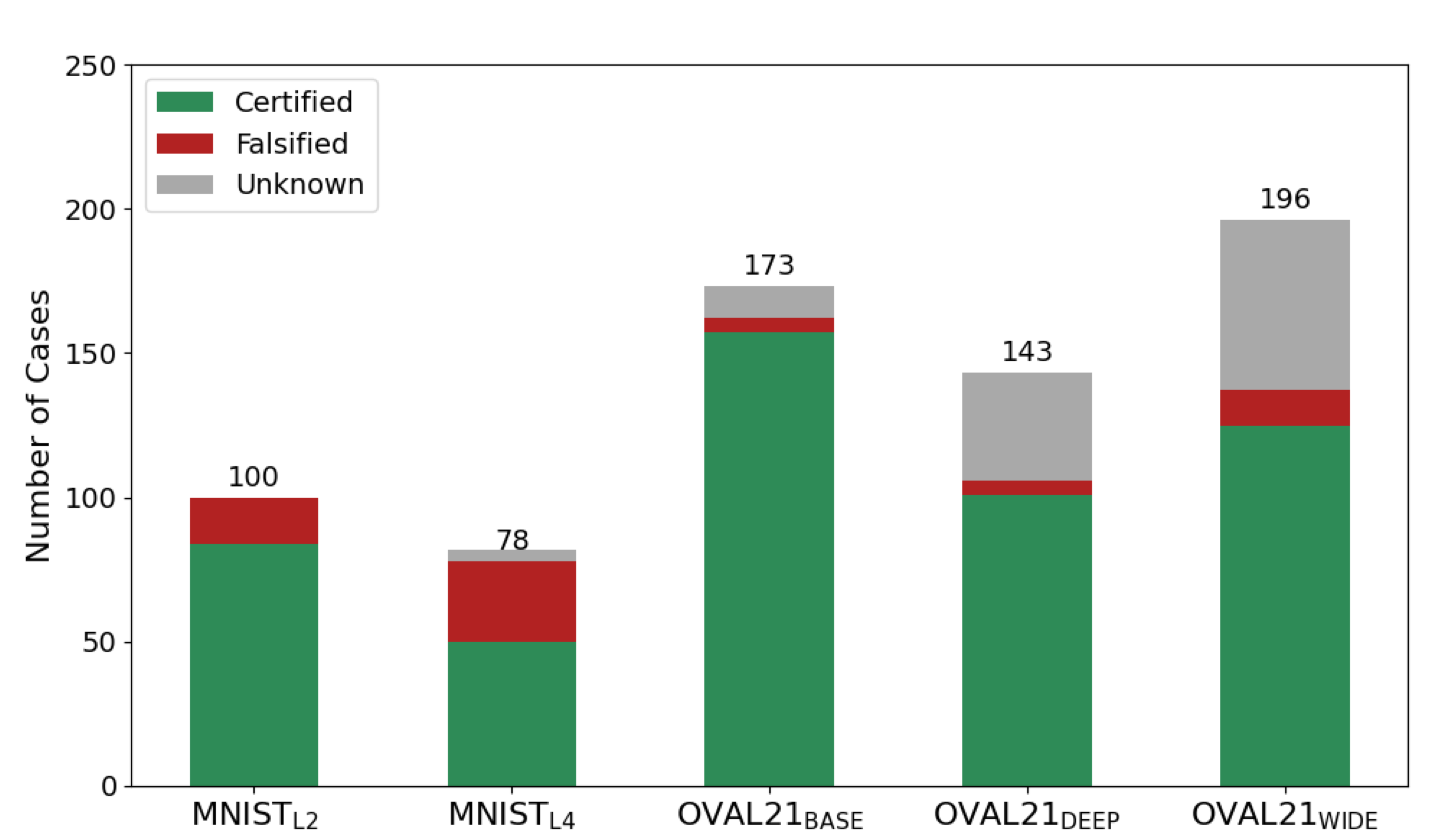
In our experiments, all our neural network models are used for image classification tasks, and all the specifications adopted are about local robustness of the neural network models. Each input specification defines an $ϵ$ as the threshold for perturbation; and each output specification requires the expected label to be matched by the original input of the model. In total, we collected 690 problem instances. Table 1 under the column “# Instances” displays the number of instances in each model, and “# Images” shows the number of different images covered by the different instances. Fig. 3 demonstrates the distribution of verification verdicts across the five models in our benchmark set, according to our experimental results. The green portion denotes tasks eventually verified (“Certified”), the red portion denotes tasks that were shown to violate the property (“Falsified”), and the gray portion corresponds to tasks that remained inconclusive (“Unknown”).

In order to present a meaningful comparison, we need to avoid the verification problems that are too simple, for which the problem can be solved within a small number of problem splitting and so there is no need to expand the $\mathrm{𝙱𝚊𝙱}$ tree too much. To that end, we perform a selection of parameters (i.e., $ϵ$ in Def. 2) of input specifications, from a range of $0/255$ to $16/255$ under the $L_{\mathrm{\infty }}$ norm. Our approach involves a binary search-like algorithm to determine the proper perturbation values for each image, as follows:

1. 1.

   Initially, we set $0/255$ as the lower bound $l$ and $16/255$ as the upper bound $u$, and calculates the midpoint by taking $m=\frac{l+u}{2}$;

2. 2.

   We apply $\mathrm{𝙱𝚊𝙱}$-baseline to the verification problem with $m$ as the $ϵ$, and check the number of nodes in the $\mathrm{𝙱𝚊𝙱}$ tree. If the tree size is greater than 1, we accept it as a candidate parameter and move to the next image; otherwise, based on the results of verification, we proceed to update $m$ as like Step 1 and repeat Step 2 as follows:

   • $\mathrm{■}$

     If the specification is violated, it implies that $ϵ$ is too large and so we set $u$ to be $m$, and update $m$ accordingly;

   • $\mathrm{■}$

     If the specification is satisfied, it implies that $ϵ$ is too small and so we set $l$ to be $m$, and update $m$ accordingly.

This process continues until a pre-defined budget is exhausted.

Fig. 4 shows the distribution of node counts across all models for the verification instances. The distribution confirms that all instances involve multiple tree nodes, ensuring meaningful sub-problem selection. Notably, more than half of the tree sizes fall within the range of 100-1000 nodes, highlighting the importance of effective sub-problem selection. The complexity of most instances necessitates careful choice in verification instances.

All experiments were conducted on an AWS EC2 instance running a Linux system with 16GB of memory and an 8-core Xeon E5 2.90 GHz CPU. All tools are developed in Python 3.9, and we used the GUROBI solver 9.1.2 [19] for the LP-based optimization. For each verification instance, we set a time budget as 1000 seconds which is consistent with VNN-COMP [30].

In Table 2, we compare the performance of our approach with the state-of-the-art baseline approaches, $\mathrm{𝙱𝚊𝙱}$-baseline, $\alpha \beta$-Crown and NeuralSAT, across all our verification problems.

We observe that, $\mathrm{𝖮𝗅𝗂𝗏𝖺}$ shows evident improvement for benchmarks including ${\text{OVAL21}}_{\text{BASE}}$, ${\text{OVAL21}}_{\text{DEEP}}$ and ${\text{OVAL21}}_{\text{WIDE}}$. On the ${\text{OVAL21}}_{\text{BASE}}$, ${\mathrm{𝖮𝗅𝗂𝗏𝖺}}^{\mathrm{𝖲𝖠}}$ solves 159 instances in an average of 155.29 seconds, far surpassing $\mathrm{𝙱𝚊𝙱}$-baseline (42 instances in 770.7 seconds) and $\alpha \beta$-Crown (58 instances in 641.7 seconds). For ${\text{OVAL21}}_{\text{DEEP}}$, ${\mathrm{𝖮𝗅𝗂𝗏𝖺}}^{\mathrm{𝖦𝖱}}$ solves 92 instances, compared to 33 by $\mathrm{𝙱𝚊𝙱}$-baseline and 55 by $\alpha \beta$-Crown, while using less time (250.72 seconds compared to 552.24 seconds). The difference is even more pronounced for ${\text{OVAL21}}_{\text{WIDE}}$, where ${\mathrm{𝖮𝗅𝗂𝗏𝖺}}^{\mathrm{𝖦𝖱}}$ solves 131 instances in an average of 240.16 seconds, greatly exceeding both $\mathrm{𝙱𝚊𝙱}$-baseline (40 instances in 733.73 seconds) and $\alpha \beta$-Crown (63 instances in 557.51 seconds).

For ${\text{MNIST}}_{\text{L2}}$ benchmarks that have simpler architectures compared to OVAL21, $\mathrm{𝙱𝚊𝙱}$-baseline performs well with 96 instances solved, while ${\mathrm{𝖮𝗅𝗂𝗏𝖺}}^{\mathrm{𝖦𝖱}}$ achieves 99 solved instances with a faster average time (57.76 seconds). As the size of the network increases to ${\text{MNIST}}_{\text{L4}}$, $\alpha \beta$-Crown declines to 44 instances, while ${\mathrm{𝖮𝗅𝗂𝗏𝖺}}^{\mathrm{𝖦𝖱}}$ achieves 67 solved instances with an average time of 146.31 seconds. These results highlight the effectiveness and efficiency of $\mathrm{𝖮𝗅𝗂𝗏𝖺}$, compared to the baseline approaches.

Table 3 presents a pairwise comparison, in which each cell indicates the number of problem instances solved by the approach listed in the row, but not solved by the approach listed in the column. Namely, we can perform pairwise comparison between two approaches by comparing the values in a pair of cells symmetric to the diagonal of Table 3. Compared to baseline approaches, our approaches demonstrate superior performances, as indicated by the green area that shows the number of additional problems solved by our approaches by not by baseline approaches; in comparison, the numbers in the red area, that includes the number of problems solved by baseline approaches, but not solved by our approaches, are much less. By comparing the performances between ${\mathrm{𝖮𝗅𝗂𝗏𝖺}}^{\mathrm{𝖦𝖱}}$ and ${\mathrm{𝖮𝗅𝗂𝗏𝖺}}^{\mathrm{𝖲𝖠}}$, we find that ${\mathrm{𝖮𝗅𝗂𝗏𝖺}}^{\mathrm{𝖦𝖱}}$ slightly outperforms ${\mathrm{𝖮𝗅𝗂𝗏𝖺}}^{\mathrm{𝖲𝖠}}$, in that it solves 40 additional problems than ${\mathrm{𝖮𝗅𝗂𝗏𝖺}}^{\mathrm{𝖲𝖠}}$, although there are 11 problems ${\mathrm{𝖮𝗅𝗂𝗏𝖺}}^{\mathrm{𝖲𝖠}}$ solves but ${\mathrm{𝖮𝗅𝗂𝗏𝖺}}^{\mathrm{𝖦𝖱}}$ does not do. That said, it also demonstrates the complementary strengths between different approaches, namely, there is no one global optimal approach that can solve all the problems, and so it is worthwhile to try different approaches when one approach does not work.

In Fig. 5, we take a further comparison between $\mathrm{𝖮𝗅𝗂𝗏𝖺}$ and $\mathrm{𝙱𝚊𝙱}$-baseline, and draw a scatter plot to show the individual instances for which $\mathrm{𝖮𝗅𝗂𝗏𝖺}$ outperform $\mathrm{𝙱𝚊𝙱}$-baseline. The $x$-axis represents the time taken by the $\mathrm{𝙱𝚊𝙱}$-baseline method in seconds, while the y-axis shows the speedup ratio of $\mathrm{𝖮𝗅𝗂𝗏𝖺}$ over $\mathrm{𝙱𝚊𝙱}$-baseline. This ratio is calculated as ${\tau }_{\mathrm{𝙱𝚊𝙱}}\left(i\right)/{\tau }_{\mathrm{𝖮𝗅𝗂𝗏𝖺}}\left(i\right)$, where ${\tau }_{\mathrm{𝙱𝚊𝙱}}(i)$ and ${\tau }_{\mathrm{𝖮𝗅𝗂𝗏𝖺}}(i)$ denote the time taken by $\mathrm{𝙱𝚊𝙱}$-baseline and $\mathrm{𝖮𝗅𝗂𝗏𝖺}$ on the instance $i$, respectively. The blue dots and orange crosses represent all of the individual problem instances. The red line is the threshold at 1$\times$ speedup, above which the ratio distinguishes that $\mathrm{𝖮𝗅𝗂𝗏𝖺}$ outperforms than $\mathrm{𝙱𝚊𝙱}$-baseline.

Across all the models, it can be seen that a significant number of blue dots (${\mathrm{𝖮𝗅𝗂𝗏𝖺}}^{\mathrm{𝖦𝖱}}$) and orange crosses (${\mathrm{𝖮𝗅𝗂𝗏𝖺}}^{\mathrm{𝖲𝖠}}$) appear above the red line, indicating that $\mathrm{𝖮𝗅𝗂𝗏𝖺}$ outperforms the $\mathrm{𝙱𝚊𝙱}$-baseline. Notably, around the 1000-second mark on the $x$-axis, there are multiple instances where the speedup ratio is up to $80\times$, meaning that $\mathrm{𝖮𝗅𝗂𝗏𝖺}$ can solve these problems more than 80 times faster than the $\mathrm{𝙱𝚊𝙱}$-baseline. This trend is particularly evident in OVAL21 models (${\text{OVAL21}}_{\text{BASE}}$, ${\text{OVAL21}}_{\text{DEEP}}$, and ${\text{OVAL21}}_{\text{WIDE}}$) that have relatively complex architectures.

In Table 4, we summarize the statistical information of speedup ratios of our approaches over $\mathrm{𝙱𝚊𝙱}$-baseline. Overall, the two variants of $\mathrm{𝖮𝗅𝗂𝗏𝖺}$ achieve consistent performance improvements, with median speedups exceeding 2 times and mean gain values around 7 times.

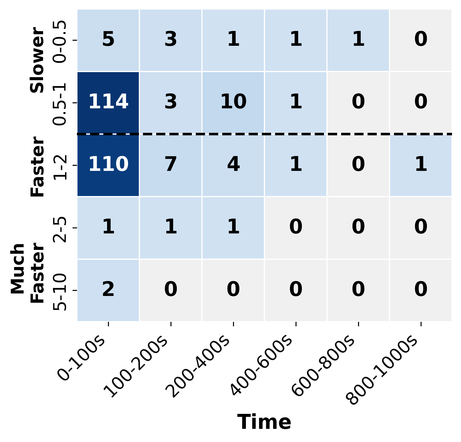
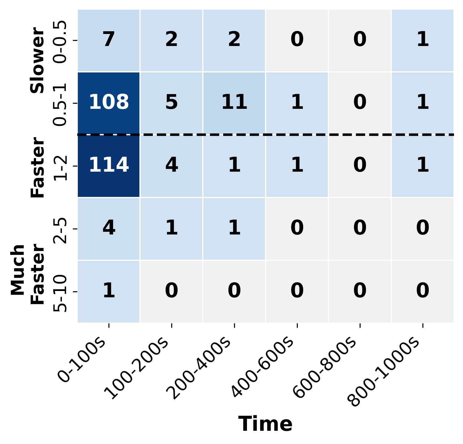
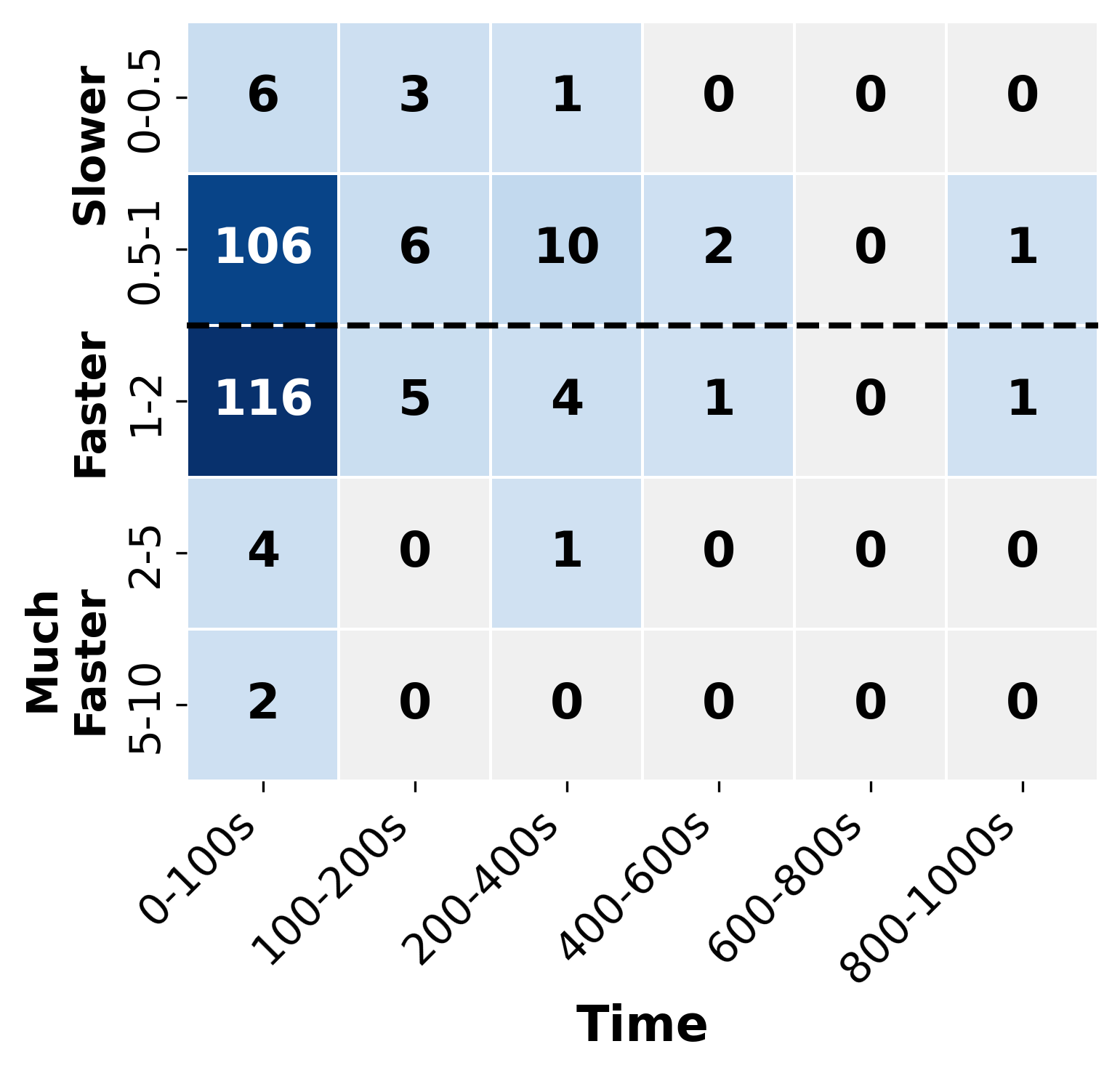
Similar to simulated annealing, our tool ${\mathrm{𝖮𝗅𝗂𝗏𝖺}}^{\mathrm{𝖲𝖠}}$ is a stochastic approach that is subject to randomness. To analyze the impact of randomness on the performance of ${\mathrm{𝖮𝗅𝗂𝗏𝖺}}^{\mathrm{𝖲𝖠}}$, we conduct five independent attempts with all the verification problems and compare them with the deterministic ${\mathrm{𝖮𝗅𝗂𝗏𝖺}}^{\mathrm{𝖦𝖱}}$. Since ${\mathrm{𝖮𝗅𝗂𝗏𝖺}}^{\mathrm{𝖲𝖠}}$ incorporates a simulated annealing approach that makes probabilistic decisions during sub-problem exploration, different runs may explore the verification space in different orders, potentially leading to variations in performance.

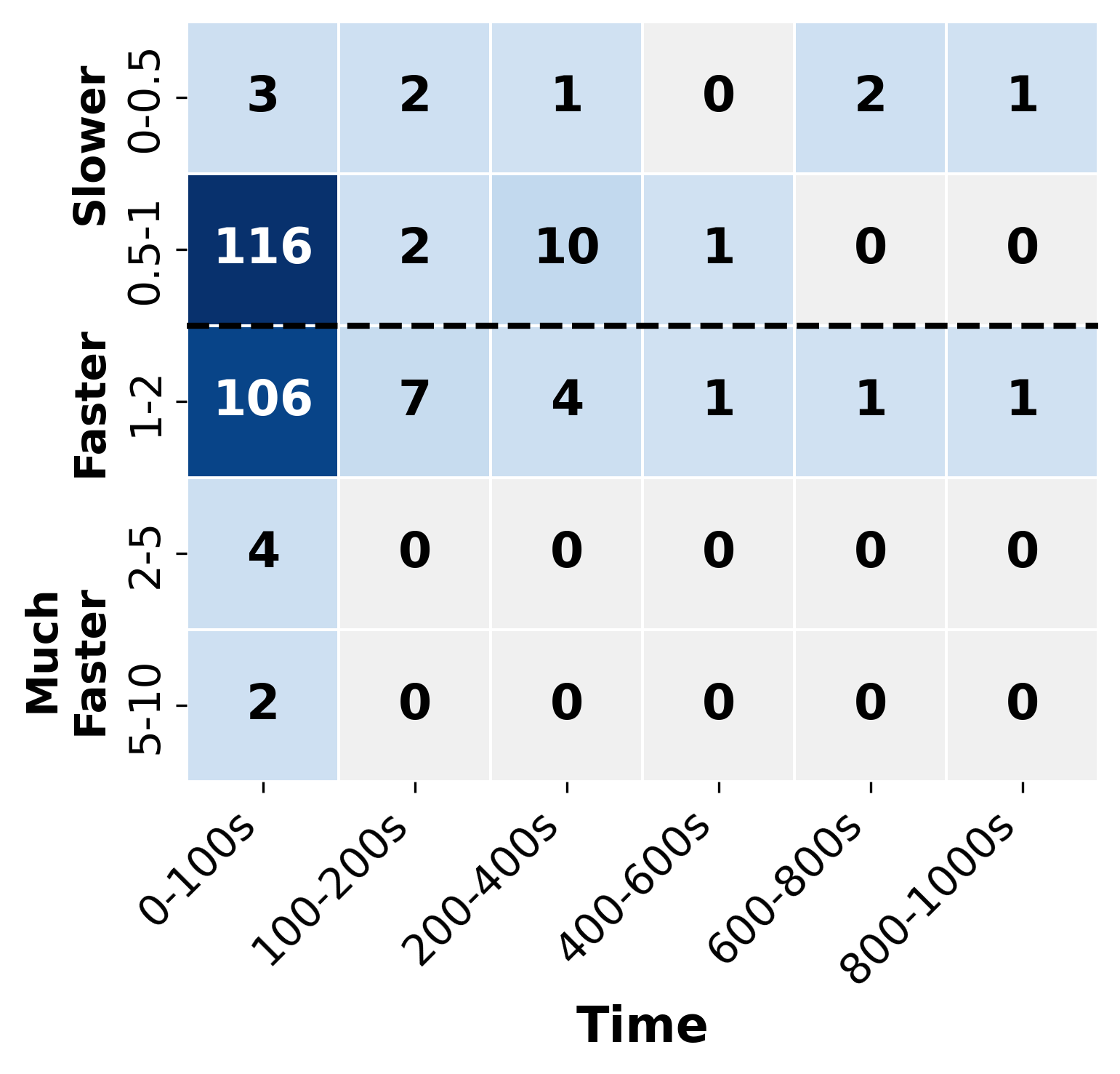
The results are presented in Fig. 6, in which we only present the problems that are either solved by ${\mathrm{𝖮𝗅𝗂𝗏𝖺}}^{\mathrm{𝖦𝖱}}$ or ${\mathrm{𝖮𝗅𝗂𝗏𝖺}}^{\mathrm{𝖲𝖠}}$. Overall, the performance comparisons between ${\mathrm{𝖮𝗅𝗂𝗏𝖺}}^{\mathrm{𝖦𝖱}}$ and ${\mathrm{𝖮𝗅𝗂𝗏𝖺}}^{\mathrm{𝖲𝖠}}$ are consistent across different attempts, and are concentrated in the 0.5-2$\times$ speedup bracket. This result suggests that the randomness in the simulated annealing approach does not substantially impact the effectiveness of ${\mathrm{𝖮𝗅𝗂𝗏𝖺}}^{\mathrm{𝖲𝖠}}$. Notably, in Fig 6(c) and Fig 6(d), with the nature of the randomness, ${\mathrm{𝖮𝗅𝗂𝗏𝖺}}^{\mathrm{𝖲𝖠}}$ exhibits the strength in finding solutions in the time cost of 100-600s that might be difficult to solve by the deterministic approach of ${\mathrm{𝖮𝗅𝗂𝗏𝖺}}^{\mathrm{𝖦𝖱}}$.

Fig. 7 shows the performance advantage of ${\mathrm{𝖮𝗅𝗂𝗏𝖺}}^{\mathrm{𝖦𝖱}}$ and ${\mathrm{𝖮𝗅𝗂𝗏𝖺}}^{\mathrm{𝖲𝖠}}$ over $\mathrm{𝙱𝚊𝙱}$-baseline across different verification tasks. For violated instances (i.e., confirmed counterexample by $\mathrm{𝙱𝚊𝙱}$-baseline and $\mathrm{𝖮𝗅𝗂𝗏𝖺}$), ${\mathrm{𝖮𝗅𝗂𝗏𝖺}}^{\mathrm{𝖦𝖱}}$ and ${\mathrm{𝖮𝗅𝗂𝗏𝖺}}^{\mathrm{𝖲𝖠}}$ consistently demonstrate superior efficiency, evidenced by lower median time costs and smaller interquartile ranges across all models.

In Fig. 7(a), $\mathrm{𝖮𝗅𝗂𝗏𝖺}$ shows notably lower median time costs and compressed interquartile ranges compared to $\mathrm{𝙱𝚊𝙱}$-baseline, indicating more consistent and faster execution. In ${\text{OVAL21}}_{\text{BASE}}$ and ${\text{OVAL21}}_{\text{DEEP}}$ (Fig. 7(c) and Fig. 7(d)), ${\mathrm{𝖮𝗅𝗂𝗏𝖺}}^{\mathrm{𝖦𝖱}}$ and ${\mathrm{𝖮𝗅𝗂𝗏𝖺}}^{\mathrm{𝖲𝖠}}$ sub-problem selection strategy is highly effective in problem instances where counterexamples exist. For ${\text{OVAL21}}_{\text{BASE}}$, ${\mathrm{𝖮𝗅𝗂𝗏𝖺}}^{\mathrm{𝖦𝖱}}$ achieves a median speed-up ratio of approximately 2.5$\times$ for violated instances, and ${\mathrm{𝖮𝗅𝗂𝗏𝖺}}^{\mathrm{𝖲𝖠}}$ with reaching up to 4$\times$ faster execution than $\mathrm{𝙱𝚊𝙱}$-baseline. Similarly, for ${\text{OVAL21}}_{\text{DEEP}}$, the median speed-up ratio is around 3$\times$, with peak performance showing up to 5$\times$ acceleration.

In contrast, for certified instances (i.e., confirmed robust), two variants of $\mathrm{𝖮𝗅𝗂𝗏𝖺}$ are generally on par with the $\mathrm{𝙱𝚊𝙱}$-baseline, indicating that in these cases, the performance of $\mathrm{𝖮𝗅𝗂𝗏𝖺}$ is comparable with $\mathrm{𝙱𝚊𝙱}$-baseline, which does not introduce overhead costs. This is expected, because in $\mathrm{𝙱𝚊𝙱}$, most of the time consumption is devoted to the problem solving process for each sub-problem. While our proposed approach introduces little overhead in the selection of the sub-problems to proceed with, the overhead is almost invisible.

Fig. 8 highlights the impact of the $\lambda$ parameter on the speedup of ${\mathrm{𝖮𝗅𝗂𝗏𝖺}}^{\mathrm{𝖦𝖱}}$ over $\mathrm{𝙱𝚊𝙱}$-baseline for the verification task on ${\text{OVAL21}}_{\text{WIDE}}$ model. In this experiment, we randomly select 20% of the instances, including 13 conclusive and 12 unknown cases, based on the $\mathrm{𝙱𝚊𝙱}$-baseline performance. The chosen instances are at varying levels of time consumption. This analysis examines $\lambda$ values ranging from $0.0$ to $1.0$, and summarizes the speedup ratios of ${\mathrm{𝖮𝗅𝗂𝗏𝖺}}^{\mathrm{𝖦𝖱}}$ under different $\lambda$ values. The findings reveal that, first, the performances of ${\mathrm{𝖮𝗅𝗂𝗏𝖺}}^{\mathrm{𝖦𝖱}}$ under different $\lambda$ are relatively stable, mostly outperforming $\mathrm{𝙱𝚊𝙱}$-baseline. This implies that both of the attributes, including the level of problem splitting and the verifier assessment, are effective in guiding the space exploration. Moreover, the performance slightly improves as $\lambda$ increases from $0.0$ to $0.5$, peaking at a speedup of $4.69$. Beyond $\lambda =0.5$, speedup declines, indicating $0.5$ as the optimal value. In terms of the average improvement, the speedup vary from $3.39$ to $4.69$ and is not negligible, which emphasizes the importance of careful tuning of $\lambda$ to maximize the efficiency of ${\mathrm{𝖮𝗅𝗂𝗏𝖺}}^{\mathrm{𝖦𝖱}}$ in verification tasks.

Then, we settle $\lambda =0.5$ as the default value to evaluate the temperature reduction parameter $\alpha$, which ranges from 0.95 to 0.999, as suggested by [24]. Fig. 9 compares the speedup of ${\mathrm{𝖮𝗅𝗂𝗏𝖺}}^{\mathrm{𝖲𝖠}}$ over ${\mathrm{𝖮𝗅𝗂𝗏𝖺}}^{\mathrm{𝖦𝖱}}$. The hyperparameter $\alpha$ determines the speed of “temperature” decreases during the verification processes, directly affecting the balances between exploration and exploitation. First, by the medians, we find that ${\mathrm{𝖮𝗅𝗂𝗏𝖺}}^{\mathrm{𝖲𝖠}}$ under all $\alpha$ outperform ${\mathrm{𝖮𝗅𝗂𝗏𝖺}}^{\mathrm{𝖦𝖱}}$. Specifically, with $\alpha =0.999$, ${\mathrm{𝖮𝗅𝗂𝗏𝖺}}^{\mathrm{𝖲𝖠}}$ achieves better performance than ${\mathrm{𝖮𝗅𝗂𝗏𝖺}}^{\mathrm{𝖦𝖱}}$ in average, which is a very slow cooling schedule ($\alpha$ close to 1) that allows the algorithm to thoroughly explore the search space early on before transitioning to exploitation. As $\alpha$ decreases, the temperature drops more rapidly, giving the algorithm less time to explore before converging on promising areas. The lower performance ratios seen with $\alpha =0.95-0.98$ suggest that this faster cooling schedule may be too aggressive, causing ${\mathrm{𝖮𝗅𝗂𝗏𝖺}}^{\mathrm{𝖲𝖠}}$ to commit too quickly to certain branches of the verification tree without adequately exploring alternatives. By our inspection of experimental results, the relative low mean values are caused by some specific cases, for which ${\mathrm{𝖮𝗅𝗂𝗏𝖺}}^{\mathrm{𝖲𝖠}}$ does not perform well. Notably, when selecting $\alpha =0.99$, while its mean ratio of 0.94 might seem underwhelming at a first glance, its median performance is notably strong compared to other $\alpha$ values, representing a balanced probability that allows sufficient exploration while maintaining steady progress toward exploitation. In practical verification tasks, as consistency can be as a valuable property, $\alpha =0.99$ can thus be preferable despite its lower mean ratio.

References

- [1] Greg Anderson, Shankara Pailoor, Isil Dillig, and Swarat Chaudhuri. Optimization and abstraction: a synergistic approach for analyzing neural network robustness. In Proceedings of the 40th ACM SIGPLAN conference on programming language design and implementation, pages 731–744, 2019. doi:10.1145/3314221.3314614.
- [2] R Anderson, J Huchette, C Tjandraatmadja, and JP Vielma. Strong convex relaxations and mixed-integer programming formulations for trained neural networks (2018), 1811.
- [3] Maksym Andriushchenko, Francesco Croce, Nicolas Flammarion, and Matthias Hein. Square attack: a query-efficient black-box adversarial attack via random search. In European conference on computer vision, pages 484–501. Springer, 2020. doi:10.1007/978-3-030-58592-1_29.
- [4] Rudy Bunel, Jingyue Lu, Ilker Turkaslan, Philip H. S. Torr, Pushmeet Kohli, and M. Pawan Kumar. Branch and bound for piecewise linear neural network verification. CoRR, abs/1909.06588, 2019. doi:10.48550/arXiv.1909.06588.
- [5] Rudy Bunel, P Mudigonda, Ilker Turkaslan, Philip Torr, Jingyue Lu, and Pushmeet Kohli. Branch and bound for piecewise linear neural network verification. Journal of Machine Learning Research, 21(2020), 2020. URL: https://jmlr.org/papers/v21/19-468.html.
- [6] Nicholas Carlini and David Wagner. Towards evaluating the robustness of neural networks. In 2017 ieee symposium on security and privacy (sp), pages 39–57. Ieee, 2017. doi:10.1109/SP.2017.49.
- [7] Chih-Hong Cheng, Georg Nührenberg, and Harald Ruess. Maximum resilience of artificial neural networks. In Deepak D’Souza and K. Narayan Kumar, editors, Automated Technology for Verification and Analysis, pages 251–268. Springer Int. Publishing, 2017. doi:10.1007/978-3-319-68167-2_18.
- [8] Moumita Das, Rajarshi Ray, Swarup Kumar Mohalik, and Ansuman Banerjee. Fast falsification of neural networks using property directed testing. arXiv preprint arXiv:2104.12418, 2021. doi:10.48550/arXiv.2104.12418.
- [9] Sumanth Dathathri, Krishnamurthy Dvijotham, Alexey Kurakin, Aditi Raghunathan, Jonathan Uesato, Rudy R Bunel, Shreya Shankar, Jacob Steinhardt, Ian Goodfellow, Percy S Liang, et al. Enabling certification of verification-agnostic networks via memory-efficient semidefinite programming. Advances in Neural Information Processing Systems, 33:5318–5331, 2020.
- [10] Alessandro De Palma, Rudy Bunel, Alban Desmaison, Krishnamurthy Dvijotham, Pushmeet Kohli, Philip HS Torr, and M Pawan Kumar. Improved branch and bound for neural network verification via lagrangian decomposition. arXiv preprint arXiv:2104.06718, 2021.
- [11] Hai Duong, Linhan Li, ThanhVu Nguyen, and Matthew B. Dwyer. A DPLL(T) framework for verifying deep neural networks. CoRR, abs/2307.10266, 2023. doi:10.48550/arXiv.2307.10266.
- [12] Hai Duong, Dong Xu, ThanhVu Nguyen, and Matthew B Dwyer. Harnessing neuron stability to improve dnn verification. Proceedings of the ACM on Software Engineering, 1(FSE):859–881, 2024. doi:10.1145/3643765.
- [13] Krishnamurthy Dj Dvijotham, Robert Stanforth, Sven Gowal, Chongli Qin, Soham De, and Pushmeet Kohli. Efficient neural network verification with exactness characterization. In Uncertainty in artificial intelligence, pages 497–507. PMLR, 2020.
- [14] Ruediger Ehlers. Formal verification of piece-wise linear feed-forward neural networks. In Automated Technology for Verification and Analysis: 15th Int. Symp., ATVA 2017, Proceedings 15, pages 269–286. Springer, October 2017.
- [15] Mahyar Fazlyab, Manfred Morari, and George J Pappas. Safety verification and robustness analysis of neural networks via quadratic constraints and semidefinite programming. IEEE Transactions on Automatic Control, 67(1):1–15, 2020.
- [16] Claudio Ferrari, Mark Niklas Muller, Nikola Jovanovic, and Martin Vechev. Complete verification via multi-neuron relaxation guided branch-and-bound. arXiv preprint arXiv:2205.00263, 2022. doi:10.48550/arXiv.2205.00263.
- [17] Xiang Gao, Ripon K Saha, Mukul R Prasad, and Abhik Roychoudhury. Fuzz testing based data augmentation to improve robustness of deep neural networks. In Proceedings of the acm/ieee 42nd international conference on software engineering, pages 1147–1158, 2020. doi:10.1145/3377811.3380415.
- [18] Ian J. Goodfellow, Jonathon Shlens, and Christian Szegedy. Explaining and harnessing adversarial examples. In 3rd Int. Conf. on Learning Representations (ICLR’15), San Diego, CA, United States, 2015. Int. Conf. on Learning Representations, ICLR.
- [19] Gurobi Optimization, LLC. Gurobi Optimizer Reference Manual, 2023. URL: https://www.gurobi.com.
- [20] Karthik Hanumanthaiah and Samik Basu. Iterative counter-example guided robustness verification for neural networks. In International Symposium on AI Verification, pages 179–187. Springer, 2024. doi:10.1007/978-3-031-65112-0_9.
- [21] Patrick Henriksen and Alessio Lomuscio. Deepsplit: An efficient splitting method for neural network verification via indirect effect analysis. In IJCAI, pages 2549–2555, 2021. doi:10.24963/ijcai.2021/351.
- [22] Xiaowei Huang, Marta Kwiatkowska, Sen Wang, and Min Wu. Safety verification of deep neural networks. In Computer Aided Verification: 29th Int. Conf., CAV 2017, Part I 30, pages 3–29. Springer, July 2017. doi:10.1007/978-3-319-63387-9_1.
- [23] Guy Katz, Clark Barrett, David L Dill, Kyle Julian, and Mykel J Kochenderfer. Reluplex: An efficient SMT solver for verifying deep neural networks. In Rupak Majumdar and Viktor Kunčak, editors, Computer Aided Verification, pages 97–117. Springer Int. Publishing, 2017. doi:10.1007/978-3-319-63387-9_5.
- [24] Scott Kirkpatrick, C Daniel Gelatt Jr, and Mario P Vecchi. Optimization by simulated annealing. science, 220(4598):671–680, 1983. doi:10.1126/science.220.4598.671.
- [25] Changliu Liu, Tomer Arnon, Christopher Lazarus, Christopher Strong, Clark Barrett, Mykel J Kochenderfer, et al. Algorithms for verifying deep neural networks. Foundations and Trends® in Optimization, 4(3-4):244–404, 2021. doi:10.1561/2400000035.
- [26] Jingyue Lu and M Pawan Kumar. Neural network branching for neural network verification. arXiv preprint arXiv:1912.01329, 2019. arXiv:1912.01329.
- [27] Zhongkui Ma, Jiaying Li, and Guangdong Bai. Relu hull approximation. Proceedings of the ACM on Programming Languages, 8(POPL):2260–2287, 2024. doi:10.1145/3632917.
- [28] Aleksander Madry, Aleksandar Makelov, Ludwig Schmidt, Dimitris Tsipras, and Adrian Vladu. Towards deep learning models resistant to adversarial attacks. In 6th Int. Conf. on Learning Representations (ICLR’18), Vancouver, Canada, 2018.
- [29] Christoph Müller, Gagandeep Singh, Markus Püschel, and Martin T Vechev. Neural network robustness verification on gpus. CoRR, abs/2007.10868, 2020.
- [30] Mark Niklas Müller, Christopher Brix, Stanley Bak, Changliu Liu, and Taylor T Johnson. 3rd international verification of neural networks competition (VNN-COMP 2022): Summary and results. arXiv preprint arXiv:2212.10376, 2022. doi:10.48550/arXiv.2212.10376.
- [31] Mark Niklas Müller, Gleb Makarchuk, Gagandeep Singh, Markus Püschel, and Martin Vechev. Precise multi-neuron abstractions for neural network certification. arXiv preprint arXiv:2103.03638, 2021. arXiv:2103.03638.
- [32] Mark Niklas Müller, Gleb Makarchuk, Gagandeep Singh, Markus Püschel, and Martin Vechev. Prima: general and precise neural network certification via scalable convex hull approximations. ACM on Programming Languages, 6(POPL):1–33, 2022. doi:10.1145/3498704.
- [33] Augustus Odena, Catherine Olsson, David Andersen, and Ian Goodfellow. Tensorfuzz: Debugging neural networks with coverage-guided fuzzing. In International Conference on Machine Learning, pages 4901–4911. PMLR, 2019. URL: http://proceedings.mlr.press/v97/odena19a.html.
- [34] Matan Ostrovsky, Clark Barrett, and Guy Katz. An abstraction-refinement approach to verifying convolutional neural networks. In International Symposium on Automated Technology for Verification and Analysis, pages 391–396. Springer, 2022. doi:10.1007/978-3-031-19992-9_25.
- [35] Kexin Pei, Yinzhi Cao, Junfeng Yang, and Suman Jana. Deepxplore: Automated whitebox testing of deep learning systems. In 26th Symp. on Operating Systems Principles, pages 1–18, 2017. doi:10.1145/3132747.3132785.
- [36] Aditi Raghunathan, Jacob Steinhardt, and Percy S Liang. Semidefinite relaxations for certifying robustness to adversarial examples. Advances in neural information processing systems, 31, 2018.
- [37] Vicenc Rubies-Royo, Roberto Calandra, Dusan M Stipanovic, and Claire Tomlin. Fast neural network verification via shadow prices. arXiv preprint arXiv:1902.07247, 2019. arXiv:1902.07247.
- [38] Zhouxing Shi, Qirui Jin, Zico Kolter, Suman Jana, Cho-Jui Hsieh, and Huan Zhang. Neural network verification with branch-and-bound for general nonlinearities. arXiv preprint arXiv:2405.21063, 2024. doi:10.48550/arXiv.2405.21063.
- [39] Zhouxing Shi, Yihan Wang, Huan Zhang, J Zico Kolter, and Cho-Jui Hsieh. Efficiently computing local lipschitz constants of neural networks via bound propagation. Advances in Neural Information Processing Systems, 35:2350–2364, 2022.
- [40] Gagandeep Singh, Rupanshu Ganvir, Markus Püschel, and Martin Vechev. Beyond the single neuron convex barrier for neural network certification. Advances in Neural Information Processing Systems, 32, 2019.
- [41] Gagandeep Singh, Timon Gehr, Matthew Mirman, Markus Püschel, and Martin Vechev. Fast and effective robustness certification. In Advances in Neural Information Processing Systems, volume 31, 2018.
- [42] Gagandeep Singh, Timon Gehr, Matthew Mirman, Markus Püschel, and Martin Vechev. Fast and effective robustness certification. Advances in neural information processing systems, 31, 2018. URL: https://proceedings.neurips.cc/paper/2018/hash/f2f446980d8e971ef3da97af089481c3-Abstract.html.
- [43] Gagandeep Singh, Timon Gehr, Markus Püschel, and Martin Vechev. Boosting robustness certification of neural networks. In Int. Conf. on learning representations, 2018.
- [44] Gagandeep Singh, Timon Gehr, Markus Püschel, and Martin Vechev. An abstract domain for certifying neural networks. ACM on Programming Languages, 3(POPL):1–30, 2019. doi:10.1145/3290354.
- [45] Yuchi Tian, Kexin Pei, Suman Jana, and Baishakhi Ray. Deeptest: Automated testing of deep-neural-network-driven autonomous cars. In 40th Int. Conf. on Software Engineering, pages 303–314, 2018. doi:10.1145/3180155.3180220.
- [46] Christian Tjandraatmadja, Ross Anderson, Joey Huchette, Will Ma, Krunal Kishor Patel, and Juan Pablo Vielma. The convex relaxation barrier, revisited: Tightened single-neuron relaxations for neural network verification. Advances in Neural Information Processing Systems, 33:21675–21686, 2020.
- [47] Vincent Tjeng, Kai Y Xiao, and Russ Tedrake. Evaluating robustness of neural networks with mixed integer programming. In Int. Conf. on Learning Representations, 2018.
- [48] Shubham Ugare, Debangshu Banerjee, Sasa Misailovic, and Gagandeep Singh. Incremental verification of neural networks. ACM on Programming Languages, 7(PLDI):1920–1945, 2023. doi:10.1145/3591299.
- [49] Shiqi Wang, Kexin Pei, Justin Whitehouse, Junfeng Yang, and Suman Jana. Efficient formal safety analysis of neural networks. Advances in neural information processing systems, 31, 2018. URL: https://proceedings.neurips.cc/paper/2018/hash/2ecd2bd94734e5dd392d8678bc64cdab-Abstract.html.
- [50] Shiqi Wang, Kexin Pei, Justin Whitehouse, Junfeng Yang, and Suman Jana. Formal security analysis of neural networks using symbolic intervals. In 27th USENIX Security Symp. (USENIX Security 18), pages 1599–1614, 2018. URL: https://www.usenix.org/conference/usenixsecurity18/presentation/wang-shiqi.
- [51] Shiqi Wang, Huan Zhang, Kaidi Xu, Xue Lin, Suman Jana, Cho-Jui Hsieh, and J Zico Kolter. Beta-crown: Efficient bound propagation with per-neuron split constraints for neural network robustness verification. Advances in Neural Information Processing Systems, 34:29909–29921, 2021. URL: https://proceedings.neurips.cc/paper/2021/hash/fac7fead96dafceaf80c1daffeae82a4-Abstract.html.
- [52] Haoze Wu, Omri Isac, Aleksandar Zeljic, Teruhiro Tagomori, Matthew L. Daggitt, Wen Kokke, Idan Refaeli, Guy Amir, Kyle Julian, Shahaf Bassan, Pei Huang, Ori Lahav, Min Wu, Min Zhang, Ekaterina Komendantskaya, Guy Katz, and Clark W. Barrett. Marabou 2.0: A versatile formal analyzer of neural networks. In Arie Gurfinkel and Vijay Ganesh, editors, Computer Aided Verification - 36th International Conference, CAV 2024, Montreal, QC, Canada, July 24-27, 2024, Proceedings, Part II, volume 14682 of Lecture Notes in Computer Science, pages 249–264. Springer, Springer, 2024. doi:10.1007/978-3-031-65630-9_13.
- [53] Cihang Xie, Zhishuai Zhang, Yuyin Zhou, Song Bai, Jianyu Wang, Zhou Ren, and Alan L Yuille. Improving transferability of adversarial examples with input diversity. In Proceedings of the IEEE/CVF conference on computer vision and pattern recognition, pages 2730–2739, 2019. doi:10.1109/CVPR.2019.00284.
- [54] Xiaoyong Xue, Xiyue Zhang, and Meng Sun. kprop: Multi-neuron relaxation method for neural network robustness verification. In International Conference on Fundamentals of Software Engineering, pages 142–156. Springer, 2023. doi:10.1007/978-3-031-42441-0_11.
- [55] Pengfei Yang, Renjue Li, Jianlin Li, Cheng-Chao Huang, Jingyi Wang, Jun Sun, Bai Xue, and Lijun Zhang. Improving neural network verification through spurious region guided refinement. In Int. Conf. on Tools and Algorithms for the Construction and Analysis of Systems, pages 389–408. Springer, 2021. doi:10.1007/978-3-030-72016-2_21.
- [56] Yang Yu, Hong Qian, and Yi-Qi Hu. Derivative-free optimization via classification. In Proceedings of the AAAI Conference on Artificial Intelligence, volume 30, 2016. doi:10.1609/aaai.v30i1.10289.
- [57] Guanqin Zhang, Zhenya Zhang, H.M.N. Dilum Bandara, Shiping Chen, Jianjun Zhao, and Yulei Sui. Efficient incremental verification of neural networks guided by counterexample potentiality. Proc. ACM Program. Lang., 9(OOPSLA1), April 2025. doi:10.1145/3720417.
- [58] Huan Zhang, Shiqi Wang, Kaidi Xu, Yihan Wang, Suman Jana, Cho-Jui Hsieh, and Zico Kolter. A branch and bound framework for stronger adversarial attacks of relu networks. In International Conference on Machine Learning, pages 26591–26604. PMLR, 2022. URL: https://proceedings.mlr.press/v162/zhang22ae.html.
- [59] Huan Zhang, Tsui-Wei Weng, Pin-Yu Chen, Cho-Jui Hsieh, and Luca Daniel. Efficient neural network robustness certification with general activation functions. Advances in Neural Information Processing Systems, 31, 2018. URL: https://proceedings.neurips.cc/paper/2018/hash/d04863f100d59b3eb688a11f95b0ae60-Abstract.html.
- [60] Zhe Zhao, Yedi Zhang, Guangke Chen, Fu Song, Taolue Chen, and Jiaxiang Liu. Cleverest: accelerating cegar-based neural network verification via adversarial attacks. In International Static Analysis Symposium, pages 449–473. Springer, 2022. doi:10.1007/978-3-031-22308-2_20.