Subgraph Counting in Subquadratic Time for Bounded Degeneracy Graphs

Abstract
We study the classic problem of subgraph counting, where we wish to determine the number of occurrences of a fixed pattern graph in an input graph of vertices. Our focus is on bounded degeneracy inputs, a rich family of graph classes that also characterizes real-world massive networks. Building on the seminal techniques introduced by Chiba-Nishizeki (SICOMP 1985), a recent line of work has built subgraph counting algorithms for bounded degeneracy graphs. Assuming fine-grained complexity conjectures, there is a complete characterization of patterns for which linear time subgraph counting is possible. For every , there exists an with vertices that cannot be counted in linear time.
In this paper, we initiate a study of subquadratic algorithms for subgraph counting on bounded degeneracy graphs. We prove that when has at most vertices, subgraph counting can be done in time. As a secondary result, we give improved algorithms for counting cycles of length at most . Previously, no subquadratic algorithms were known for the above problems on bounded degeneracy graphs.
Our main conceptual contribution is a framework that reduces subgraph counting in bounded degeneracy graphs to counting smaller hypergraphs in arbitrary graphs. We believe that our results will help build a general theory of subgraph counting for bounded degeneracy graphs.
Keywords and phrases:
Homomorphism counting, Bounded degeneracy graphs, Fine-grained complexity, Subgraph countingCategory:
Track A: Algorithms, Complexity and GamesCopyright and License:
2012 ACM Subject Classification:
Mathematics of computing Graph algorithmsFunding:
Both authors are supported by NSF CCF-1740850, CCF-1839317, CCF-2402572, and DMS-2023495.Editors:
Keren Censor-Hillel, Fabrizio Grandoni, Joël Ouaknine, and Gabriele PuppisSeries and Publisher:
1 Introduction
The fundamental algorithmic problem of subgraph counting in a large input graph has a long and rich history [37, 23, 28, 21, 38, 1, 19, 42, 49]. There are applications in logic, properties of graph products, partition functions in statistical physics, database theory, machine learning, and network science [17, 15, 25, 10, 42, 22, 41]. We are given a pattern graph , and an input graph . All graphs are assumed to be simple. We use to denote the problem of computing the number of (not necessarily induced) subgraphs of in , that is, the number of subgraphs of isomorphic to .
If the pattern is part of the input, this problem becomes NP-hard, as it subsumes subgraph isomorphism. Often, one thinks of the pattern as fixed, and running times are parameterized in terms of the properties (like the size) of . Let us set and . There is a trivial brute-force algorithm, but we do not expect algorithms for general for some constant [21].
The rich field of subgraph counting focuses on restrictions on the pattern or the input, under which non-trivial algorithms and running times are possible [33, 3, 15, 24, 23, 21, 10, 19, 11, 47]. Given the practical importance of subgraph counting, there is a special focus on linear time (or small polynomial running times).
Inspired by seminal work of Chiba-Nishizeki [18], a recent line of work has focused on building a theory of subgraph counting for bounded degeneracy graphs [11, 6, 7, 14, 5]. These are classes of graphs where all subgraphs have a constant average degree. This work culminated in results of Bera-Pashanasangi-Seshadhri and Bera-Gishboliner-Levanzov-Seshadhri-Shapira [7, 5]. We now have precise dichotomy theorems characterizing linear time subgraph counting in bounded degeneracy graph. When has at most vertices, then can be determined in linear time (if has bounded degeneracy). For all , there is a pattern on vertices that cannot be counted in linear time, assuming fine-grained complexity conjectures. The following question is the next step from this line of work.
When can we get subquadratic algorithms for subgraph counting (when has bounded degeneracy)? Are there non-trivial algorithms that work for all with (or more) vertices?
Before stating our main results, we offer some justification for this problem.
Bounded degeneracy graphs.
This is an extremely rich family of graph classes, containing all non-trivial minor-closed families, bounded expansion families, and preferential attachment graphs [48]. Most massive real-world graphs, like social networks, the Internet, communication networks, etc., have low degeneracy ([30, 34, 51, 4, 8], also Table 2 in [4]). The degeneracy has a special significance in the analysis of real-world graphs, since it is intimately tied to the technique of “core decompositions” [48]. Most of the state-of-the-art practical subgraph counting algorithms use algorithmic techniques for bounded degeneracy graphs [1, 35, 42, 40, 34, 41].
Subquadratic time.
From a theoretical perspective, the orientation techniques of Chiba-Nishizeki and further results [18, 6, 7, 5] are designed for linear time algorithms. The primary technical tool is the use of DAG-Tree decompositions, introduced in a landmark result of Bressan [11, 12]. Bressan’s algorithm yields running times of the form , where and is the DAG-treewidth of . It is known that linear time algorithms are possible iff the DAG-treewidth is one [5]. It is natural to ask if the DAG-treewidth being two is a natural barrier. Subquadratic algorithms would necessarily require a new technique, other than DAG-treewidth. It would also show situations where the DAG-treewidth can be beaten.
From a practical standpoint, the best exact subgraph counting codes (the ESCAPE package [27]) use methods similar to the above results. Algorithms for bounded degeneracy graphs have been remarkably successful in dealing with modern large networks. Subquadratic algorithms could provide new practical tools for subgraph counting.
The focus on vertices and the importance of cycle patterns.
The problem of counting all patterns of a fixed size is called graphlet analysis in bioinformatics and machine learning [43, 50]. Current scalable exact counting codes go to 5 vertex patterns [27], which is precisely the theoretical barrier seen in [6]. Part of our motivation is to understand the complexity of counting all vertex patterns (in bounded degeneracy graphs).
The seminal cycle detection work of Alon-Yuster-Zwick also gave algorithms parameterized by the graph degeneracy [3]. But most of their results are for cycle detection, whereas counting is arguably the more relevant problem. It is natural to ask if counting is also feasible with similar running times.
1.1 Main Results
Our main result shows that patterns with at most vertices can be counted in subquadratic time. Let be the number of vertices and be the degeneracy of the input graph . The degeneracy is the maximum value, over all subgraphs of , of the minimum degree of the subgraph. In what follows, denote some explicit function.
Theorem 1.1 (Main Theorem).
There is an algorithm that computes111We can obtain a similar result for the problem of counting only induced subgraphs , as it can be expressed as a linear combination of for some patterns with . for all patterns with at most vertices in time .222We express our results parameterizing by the degeneracy of the input graph . Note that if is from a class with bounded degeneracy, then is constant and we can ignore that term.
Recall that previous works gave (near) linear time algorithms when had at most vertices [6]. The best subgraph counting algorithm for bounded degeneracy graphs is Bressan’s algorithm, which runs in at least quadratic (if not cubic) time for many patterns with to vertices.
Additionally, we construct an explicit -vertex pattern that we conjecture cannot be counted in subquadratic time in the bounded degeneracy setting. We are able to relate the complexity of counting that pattern to counting a specific hypergraph in general graphs, which we believe can not be done in subquadratic time. (More in §1.2.6)
1.1.1 Counting cycles
As a secondary result, we are able to show that cycle counting in bounded degeneracy graphs can be done even faster. These results are tight, in the sense that any improvement will imply beating long standing cycle detection algorithms for sparse graphs. Let denote the -cycle and be the exponent (in terms of edges) of the current fastest algorithm for -cycle detection in general graphs (see (3) and [29]). Gishboliner-Levanzov-Shapira-Yuster (henceforth GLSY) recently showed that homomorphism counting of in bounded degeneracy graphs can be done in time [29]. We prove that this complexity can be matched for the problem of subgraph counting. Cycle counting is more challenging, since it involves compute linear combinations of homomorphisms of non-cyclic patterns (which requires other techniques).
Theorem 1.2.
Let denote the degeneracy of the input graph .
-
There is an algorithm that computes and in time , where . Moreover, unless there is an -time algorithm for counting triangles for some , there is no -time algorithm for any .
-
There is an algorithm that computes and in time , where . Moreover, unless there is an -time algorithm for counting -cycles for some , there is no -time algorithm for any .
-
There is an algorithm that computes in time , where . Moreover, unless there is an -time algorithm for counting -cycles for some , there is no -time algorithm for any .
Previously, for bounded degeneracy graphs, subquadratic results were only known for detecting cycles, by a result of Alon, Yuster and Zwick [3]. Theorem 1.2 improves or matches their bounds in all cases, despite solving the harder problem of counting. The lower bounds relating to cycle counting in general graphs follow directly from the techniques of GLSY [29]. We note that the exponents have not been improved for twenty years [3, 53]. As a side corollary of our methods, we also get a better algorithm for counting -cycles in arbitrary graphs (Corollary 1.7).
1.2 Main Ideas
The theorems above are obtained from a new reduction technique that converts homomorphism counting in bounded degeneracy graphs to subgraph counting in arbitrary graphs for some specific patterns.
The starting point for most subgraph counting algorithms for bounded degeneracy graphs is to use graph orientations [48]. A graph has bounded degeneracy iff there exists an acyclic orientation such that all vertices have bounded outdegree. (An acyclic orientation is obtained by directing the edges of into a DAG.) Moreover, this orientation can be found in linear time [39]. To count -subgraphs in , we consider all possible orientations of and compute (the sum of) all .
The approach formalized by Bressan [12] and Bera-Pashanasangi-Seshadhri [6] is to break into a collection of (out)directed trees rooted at the sources of . The copies of each tree in can be enumerated in linear time, since outdegrees are bounded. We need to figure out how to “assemble” these trees into copies of .
Bressan’s DAG-tree decomposition gives a systematic method to perform this assembly, and the running time is , where is the “DAG-treewidth” of . The definition is technical, so we do not give details here. Also, this method only gives the homomorphism count (edge-preserving maps from to ), and we require further techniques to get subgraph counts [19]. The main contribution of the linear time dichotomy theorems is to completely characterize patterns such that all orientations have DAG-treewidth one [7, 5].
Since is a natural number, to get subquadratic time algorithms, we need new ideas.
1.2.1 The 6-cycle
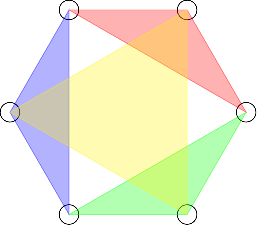
It is well-known (from [3]) that linear-time orientation based methods hit an obstruction at -cycles. Consider the oriented -cycle in the left of Fig. 1. It is basically a “triangle” of out-out wedges (as given by the red lines); indeed, one can show that -cycle counting in bounded degeneracy graphs is essentially equivalent to triangle counting in arbitrary graphs [6, 7, 5]. This observation can be converted into an algorithm, as was shown by GLSY [29]. Starting with , we create a new graph with edges (the red lines) corresponding to the endpoints of out-out wedges. Since has bounded outdegree, the number of edges in the new graph is . Every triangle in the new graph corresponds to a (directed) -cycle homomorphism in . Triangle counting in the new graph can be done in time (or time using a combinatorial algorithm) [3]. Getting the subgraph count is more involved, but we can use existing methods that reduce to homomorphism counting [19].
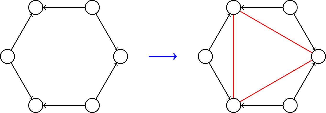
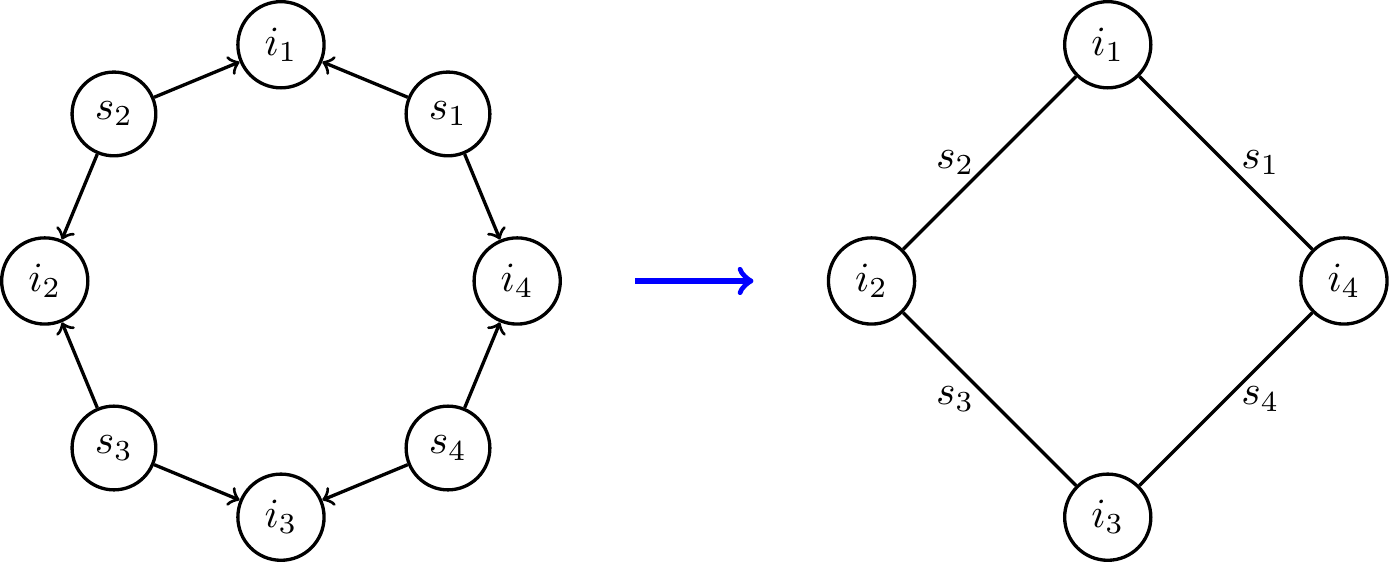
One can extend this idea more generally as follows. Let be a directed pattern, a source is any vertex with no incoming arcs, and we define an intersection vertex as any vertex that can be “reached” by two different sources.
Suppose there are sources and intersection vertices. Suppose further that there is an ordering of the sources and the intersection vertices of such that, for all , only the sources and (taking modulo in the indexes) can both reach the vertex . This is the case of the oriented and in Fig. 1 or of any acyclic orientation of any cycle. One can then construct a new graph such that is the same as (where denotes the homomorphism count).
1.2.2 Generalizing to non-cyclic patterns
So far, the algorithmic approach only makes sense for cycle patterns. Our main contribution is a framework that generalizes this approach to count homomorphisms and subgraphs of more complex patterns.
The first part of our framework is the concept of -reducible patterns. Let be a hypergraph, a directed pattern is -reducible if we can reduce counting homomorphisms of it to counting subgraphs in a sparse hypergraph. The formal definition is technical and can be seen in §3. We provide a simplified exposition in this section.
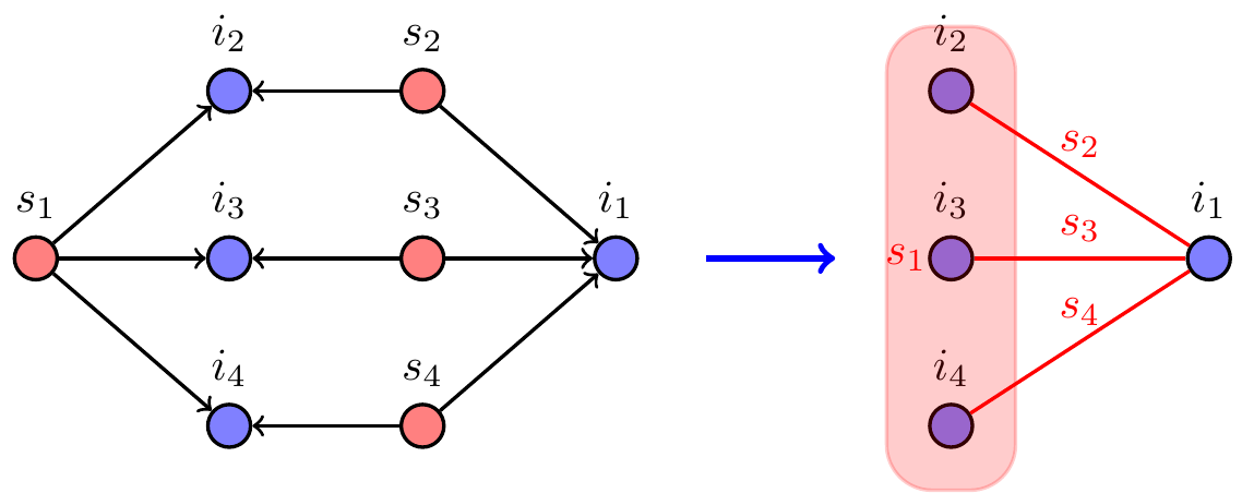
Consider a directed pattern , for example the left image in Fig. 2. We can replace every source with a hyperedge connecting the intersection vertices reachable from the source. The result is a graph (or hypergraph) such that is -reducible.
However, our framework allows for even more freedom: instead of looking at individual sources, we partition sources into sets of sources . See the rightmost figure in Fig. 2 for an example, where the sources are divided into sets of sources. The sub-patterns induced by the vertices reachable from every set of sources are “easy” to count using existing techniques. We can also arrange the intersection vertices into sets such that every set of sources will reach some sets of intersection vertices. We can obtain by replacing every set of intersection vertices with a vertex and every set of sources with a hyperedge that contains the vertices corresponding to the sets of intersection vertices that can be reached by .
In the second example of Fig. 2, the intersection of the vertices reachable from source sets forms a “cyclic arrangement”. The intersection vertices reachable from are also reachable from and , and similarly for the other sets of sources, giving that the pattern will be -reducible.
1.2.3 The reduced graph
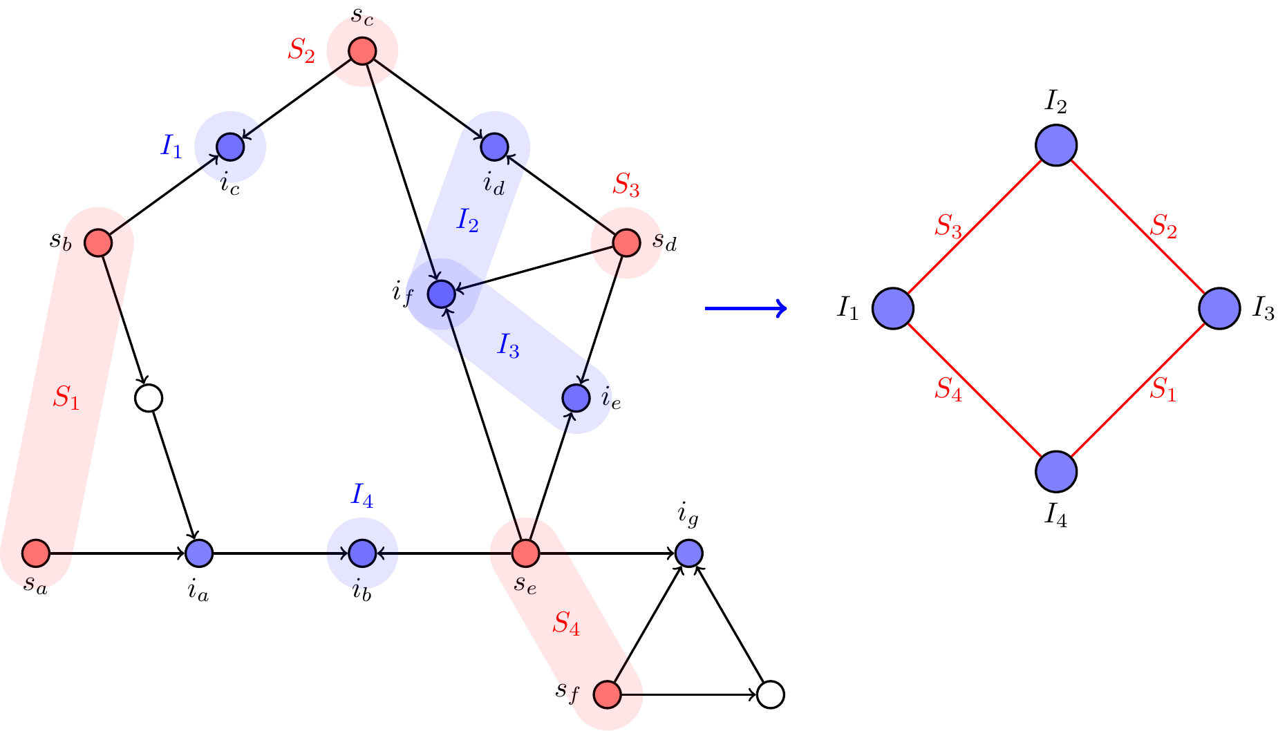
The second part of our framework is the reduced graph. If a pattern is -reducible, then for any directed input graph , we can construct a colored weighted graph with the following property. The number of homomorphisms of the original pattern relates to the number of colorful copies of in .
The reduced graph consists of layers of vertices, where each layer is related to one intersection set of . Specifically, there is a vertex in the -th layer for every possible image of the corresponding intersection set in , that is, every set of vertices in such that can be mapped to it. Moreover, the vertices of every layer will have the same color. For example, for every intersection set in and any map there is a vertex in with color .333There could be such vertices, however, as we will note later, there will be at most edges, so we can ignore vertices with degree and we do not need to even create them.
The edges have weights that represent the number of homomorphisms mapping the intersection sets to the corresponding images. For example, let be a source set reaching two intersection sets and , and let . An edge connecting and with weight indicates that there are different homomorphisms mapping (the subgraph of induced by the vertices reachable from ) to that map to and to . Additionally we can show that if has bounded outdegree, then the new reduced graph will have edges.
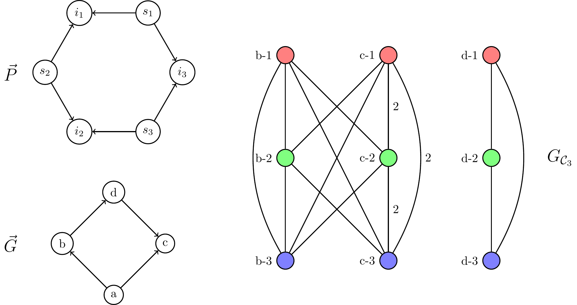
We give an example in Fig. 3. For simplicity of exposition, the graph is smaller than the pattern. Each vertex of has three copies (each with a different color) in the reduced graph, denoted . Since the vertex cannot be the image of any intersection vertex (it has zero indegree), copies of this vertex do not appear in . Observe that there is no mapping of an out-out wedge where is one endpoint and is the other endpoint. Hence, there is no edge from a copy of to a copy of .
Every colorful copy of in correspond to fixing the positions of the intersection sets in , and the weight of each hyperedge will correspond to the number of homomorphisms mapping that portion of the graph. Hence the product of the weights of all hyperedges in each copy will give the total number of homomorphisms mapping all the intersection sets to the corresponding vertices in . Therefore, the total number of homomorphisms will be equal to the quantity , which corresponds to the sum of products of weights of colorful copies of . That is:
| (1) |
Here, denotes the set of distinct colorful copies of in . We are able to show that solving is equivalent to counting the number of homomorphisms of in .
Therefore, we can count homomorphisms of -reducible patterns in the same time as counting colorful copies of in the reduced graph.
Lemma 1.3.
Let . If there exists a -time algorithm that for any graph computes , then for any -reducible pattern and directed input graph , we can compute in time , where is the maximum outdegree of .
1.2.4 From directed to undirected: getting homomorphisms counts
To extend our reduction framework to undirected graphs we introduce the concept of -computable patterns. Note that different acyclic orientations of the same pattern might reduce to different graphs. Let be a set of graphs, we say that a pattern is -computable if all the acyclic orientations of can be computed in linear time or are -reducible for some . If for all the patterns in we can compute in time then we can use Lemma 1.3 to get a bound on the complexity of .
For each , we find a set of hypergraphs such that all patterns with vertices are -computable. These sets grow with and we have . We give a definition of these sets in Section §5 and prove the following lemma.
Lemma 1.4.
Let , every connected pattern with vertices is -computable.
For we are able to show that there exists a subset of such that every -vertex pattern is also -computable and for every pattern we can compute in time. Allowing us to show that for all patterns with vertices or less we can count the number of homomorphisms in subquadratic time.
We can also show similar results for cycles. All orientations of cycle patterns can be reduced to cycles of half their length. This means that any -cycle and -cycle are -computable (in these cases we will simply write -computable).
We can also show that for all cycles we can compute in time, the fastest time for detecting -cycles in general graphs.
Lemma 1.5.
For all , there is an algorithm that computes in time .
This means that we can compute the number of homomorphisms of and in time , similar result to the one obtained in GLSY [29].
1.2.5 Getting subgraph counts
At this point, we have algorithms for computing various pattern homomorphisms. To get subgraph counts, we need the inclusion-exclusion techniques of [19]. One can express the -subgraph count as a linear combination of -homomorphism counts, where is a pattern in . The consists of all patterns such that has a surjective homomorphism to . Thus, every pattern in the spasm has at most as many vertices as .
Hence for any pattern with vertices, all the patterns in will have at most vertices and hence they will also be -computable, giving Theorem 1.1.
In the case of the cycles, to be able to extend the results from last section to the problem, we analyze the spasm of the different cycles. For we are able to show that the patterns in the spasms of are also -computable. That combined with Lemma 1.5 implies the upper bound of Theorem 1.2.
1.2.6 Inverting the reduction for conditional hardness
We show that in some cases our reduction procedure is optimal. For example, counting small cycles in general graphs can be reduced to counting cycles of twice the length in graphs of degeneracy . The reduction is quite simple and just involves subdividing the edges. With a slight modification, the subdivision approach can be used to show lower bounds for odd cycles too, which gives the lower bound of Theorem 1.2. We note that an analogous result for counting homomorphisms was shown in GLSY [29].
Lemma 1.6.
Let . For any , the existence of an -time algorithm for counting -cycles implies an -time algorithm for counting -cycles in general graphs, for some .
This inversion of the reduction procedure also gives us an algorithm for counting undirected -cycles in general graphs which improves on the current state of the art, and matches the complexity for -cycle detection.
Corollary 1.7.
There is an algorithm that, for any graph , computes in time .
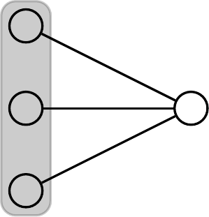
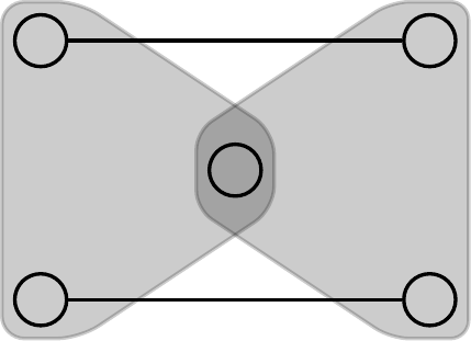
The approach of subdividing edges can be used to prove a relation between other patterns too. In the case of hypergraphs, we can replace hyperedges of arity by -stars. We are able to show a strong relation between the hypergraph depicted in Fig. 4, and a -vertex pattern. We conjecture that for this pattern we can not count the number of subgraphs in subquadratic time.
Conjecture 1.8.
For any , there is no -time algorithm for computing .
This conjecture implies that there are no subquadratic algorithms for computing the number of subgraphs of all -vertex patterns.
Lemma 1.9.
If Conjecture 1.8 holds, then for any there is no algorithm that computes in time for all patterns with vertices.
We consider it an interesting open problem to relate our conjecture with existing fine-grained complexity assumptions. Some previous works prove barriers for subquadratic listing in general graphs [16], but no similar results exist for counting hypergraphs.
1.3 Related Work
Subgraph counting is closely tied to homomorphism counting; in some cases, it is more convenient to talk about the latter. Seminal work of Curticepean-Dell-Marx showed that the optimal algorithms for subgraph counting can be designed from homomorphism counting algorithms and vice versa [19].
Much of the study of subgraph/homomorphism counting comes from paramterized complexity theory. Díaz et al [23] gave a algorithm for determining the -homomorphism count, where is the treewidth of . Dalmau and Jonsson [21] proved that is polynomial time solvable iff has bounded treewidth. Otherwise it is -complete. Roth and Wellnitz [47] consider restrictions of both and , and focus of -completeness.
Tree decompositions have played an important role in subgraph counting. We give a brief review of the graph parameters treewidth and degeneracy. The notion of tree decomposition and treewidth were introduced in a seminal work by Robertson and Seymour [44, 45, 46], although the concept was known earlier [9, 31].
Degeneracy is a measure of sparsity and has been known since the early work of Szekeres-Wilf [52]. We refer the reader to the short survey of Seshadhri [48] about degeneracy and algorithms. The degeneracy has been exploited for subgraph counting problems in many algorithmic results [18, 26, 1, 35, 42, 40, 34, 41].
Bressan connected degeneracy to treewidth-like notation and introduced the concept of DAG treewidth [11, 12]. The main result is the following. For a pattern with and an input graph with and degeneracy , one can count in time, where is the DAG treewidth of . Assuming the exponential time hypothesis [32], the subgraph counting problem does not admit any -time algorithm, for any positive function .
Bera-Pashanasangi-Seshadhri introduced the first theory of linear time homomorphism counting [6], showing that all patterns with at most vertices could be counted in linear time. It was later shown that for every pattern with no induced cycles of length or more, the number of homomorphisms could also be counted in linear time [7, 5].
A recent work of Komarath et al. [36] gave quadratic and cubic algorithms for counting cycles in sparse graphs. Gishboliner et al. gave subquadratic algorithms for homomorphism counting of cycles in bounded degeneracy graphs [29]. Bressan, Lanziger and Roth have also studied counting algorithms for directed patterns [13].
1.4 Paper Organization
In Section , we define our reduction framework formally and prove the equivalence between the bounded degeneracy and the general setting. In Section , we prove that many patterns are cycle-reducible. In Section , we define the sets and complete the proof of the main theorem. Finally, in Section , we show how to compute Col-WSub for cycle patterns. Due to space limitations most proofs have been deferred to the Full Version, including the proofs of Lemma 1.6 and Lemma 1.9.
2 Preliminaries
Graphs, subgraphs and homomorphisms
We use to denote the pattern graph and to denote the input graph. We will use and for the number of vertices and edges of respectively.
A homomorphism from to is a mapping such that we have . We use to denote the set of all homomorphisms from to . We use to denote the problem of counting the number of homomorphisms from to , that is, computing . Similarly we use to denote the problem of counting the number of subgraphs (not necessarily induced) of isomorphic to .
We say that two homomorphisms and agree if for any vertex we have .
The spasm of a graph is the set of all possible graphs obtained by recursively combining two vertices that are not connected by an edge, removing any duplicated edge. Using inclusion-exclusion arguments one can express the value of as a weighted sum of homomorphism counts of the graphs in the spasm of . Hence, computing for all , allows to compute , as given by the following equation: .
Degeneracy and directed graphs
A graph is -degenerate if every subgraph has a minimum degree of at most . The degeneracy of a graph is the minimum nonnegative value such that is -degenerate. There exists an acyclic orientation of a graph, called the degeneracy orientation, which has the property that the maximum outdegree of the graph is at most [39]. Additionally, this orientation can be computed in time. We will use to denote the directed input graph. For a pattern , we use to denote the set of acyclic orientations of . When orienting the input graph, every occurrence of will now appear as exactly one of its acyclic orientations, that is, .
We say that is a source if its in-degree is . We use to denote the set of sources of . We say a vertex is reachable from if there is a directed path connecting to and use to denote the set of vertices reachable from the source . Abusing notation, for a set we use (or if is clear from the context) to denote the set of vertices reachable from at least one vertex in . We use and for the subgraphs of induced by and .
We say that a vertex of is an intersection vertex if there are at least two distinct sources such that is reachable from both of them, that is, . We use to denote the set of intersection vertices. Note that .
The DAG-treewidth
Bressan introduced the concept of DAG-tree decomposition of a directed acyclic graph [11]:
Definition 2.1 (DAG-tree decomposition [11]).
For a given directed acyclic graph , a DAG-tree decomposition of is a rooted tree such that:
-
Each node , is a subset of the sources of , .
-
Every source of is in at least one node of , .
-
, if is in the unique path between and in , then .
The DAG-treewidth of a DAG-tree decomposition , , is the maximum size of all the bags in . The DAG-treewidth of a directed acyclic graph is the minimum value of across all valid DAG-tree decomposition of . For an undirected graph , we will have that .
Using DAG-tree decomposition to compute homomorphisms
Bressan gave an algorithm that computes making use of the DAG-tree decomposition of a directed pattern [11, 12]. The algorithm decomposes the pattern into smaller subgraphs, computes the number of homomorphisms of every subgraph and then combines the counts using dynamic programming.
Theorem 2.2 ([11]).
For any pattern with vertices there is an algorithm that computes in time .
For the patterns with we obtain an algorithm that runs in near-linear time for graphs of constant degeneracy. Bera et al. showed an exact characterization of which patterns have , which depends only on the length of the largest induced cycle of the pattern ().
Lemma 2.3 ([7]).
.
If we analyze the algorithm from Bressan in more detail, we can see that it can be used as a black box to obtain some more fine-grained counts. In order to understand this we need to introduce the following definition:
A homomorphism extends if for every vertex mapped by we have . Let be a homomorphism from a subgraph of to . We define as the number of homomorphisms from to that extend .
Lemma 2.4 (Lemma in [12] (restated)).
There exists an algorithm that, given a directed pattern with vertices and a DAG-tree decomposition rooted in with , and a directed graph with vertices and maximum outdegree ; returns, for every homomorphism , the quantity . The algorithm runs in time .
Hypergraphs
A hypergraph is a generalization of a graph where each edge (or hyperedge) is a subset of the vertex set. The arity of a hyperedge is the number of vertices that it contains. We will only consider hypergraphs where every hyperedge has arity at least . We use for the set of hyperedges of , where for each we have . We will also consider weighted hypergraphs, for a hypergraph , the function gives the weight of each hyperedge in . We use to denote the simplex hypergraph of arity , that is, the hypergraph on vertices with all possible hyperedges of arity .
3 The reduction procedure
In this section, we explain the reduction procedure underlying the notion of -reducibility. The idea is to organize the structure of the directed pattern based on the hypergraph .
First, we partition the set of sources of the directed pattern into disjoint subsets , one for each hyperedge in . Every source belongs to exactly one subset . This partition allows us to decompose into smaller subgraphs, each corresponding to a hyperedge, where the subgraphs can be efficiently counted using Bressan’s algorithm.
Second, we associate to each vertex a subset of intersection vertices . Not all the intersection vertices need to belong to one of the subsets; we let denote the set of intersection vertices that appear in at least one . A given intersection vertex may belong to multiple subsets, but we require that the vertices of corresponding to all subsets containing a common intersection vertex induce a connected subgraph.
To connect the sources to the intersection vertices, we define, for each hyperedge , the set as the subset of reachable from the sources in . We require that the sources in reach all the intersection vertices assigned to the vertices incident to . Moreover, for each vertex , the sources associated with any hyperedge containing must reach all the vertices in .
These conditions ensure that we can correctly combine the homomorphism counts for each subgraph to compute the homomorphism counts of . We now present the full formal definition.
Definition 3.1 (-reducible).
A connected DAG is -reducible if there exist subsets for every vertex , and subsets for every hyperedge , satisfying the following conditions:
-
Let . For every intersection vertex , the set of vertices induces a connected hypergraph in .
-
The subsets are disjoint, i.e., for all , and they cover all sources, i.e., .
-
For every hyperedge , the subset contains a source such that , and the subgraph admits a DAG-tree decomposition rooted at .
-
For every vertex and every hyperedge containing , we have .
-
For every hyperedge , we have .
We now define the reduced graph .
Definition 3.2 (Reduced graph ).
Given a -reducible directed pattern on source sets and intersection sets , we define the reduced graph of the directed input graph as follows:
-
For every vertex and every homomorphism we have the vertex with color . The vertices with the same color form the “layers” of .
-
For every hyperedge and for every homomorphism , let be the restriction of to for each vertex , we will have a hyperedge connecting the vertices with weight .
We use to refer to the vertices of in the -th layer. The number of vertices in every layer can be up to , however we will only consider vertices that are not isolated, that is, have degree at least . We can show that we can construct efficiently when only considering such vertices.
Lemma 3.3.
Given a -reducible pattern and a directed graph with maximum outdegree , we can construct in time. Additionally, the number of non-isolated vertices and the total number of hyperedges are bounded by .
We can now prove the equivalence between homomorphisms of the original pattern and weighted colorful copies of the reduced hypergraph. This lemma relates the counts between the original and the reduced graph.
Lemma 3.4.
Finally, we have all the tools to complete our reduction framework, giving us Lemma 1.3.
See 1.3
Proof.
3.1 From directed to undirected
We introduce the concept of -computable, which will help us give upper bounds in the complexity of undirected patterns.
Definition 3.5 (-computable).
Let be a set of hypergraphs. We say that a pattern is -computable if every acyclic orientation has either DAG-treewidth of or there exists a hypergraph such that is -reducible.
If a pattern is -computable and is only formed by cyclic patterns we will instead write -computable, where is the length of the largest cycle in . The complexity of computing homomorphisms of -computable patterns will be dominated by the hardest complexity for computing .
Lemma 3.6.
Let be a set of hypergraphs, if for every hypergraph there is an algorithm that computes in time , then for any input graph with degeneracy and any -computable pattern , there is an algorithm that computes in time .
4 Reducing to cycles
We first focus on patterns that can be reduced to counting cycles. We start by introducing the following two lemmas, showing that directed patterns with either few sources or few intersection vertices are -reducible.
Lemma 4.1.
Every directed acyclic pattern with at most sources is either -reducible or .
Lemma 4.2.
Every directed acyclic pattern with at most intersection vertices is either -reducible or .
Using this two lemmas we can prove that all and -vertex patterns are -computable.
Lemma 4.3.
Every and -vertex undirected pattern is -computable.
Additionally, the patterns in the spasm will always have less vertices, and hence all patterns in the spasms of all and -vertex patterns will also be -computable. This fact, together with Lemma 1.5 gives the following.
Corollary 4.4.
Let be a pattern with or vertices. For any input graph , we can compute and in time .
We can also show that the acyclic orientations of cycle patterns are always -reducible for some at most half of the length of the cycle. This is equivalent to the result in [29], but expressed using our reducibility framework.
Lemma 4.5.
For all , and are -computable.
Moreover, we can also show that all patterns in the spasms of cycles up to length are also cycle-computable.
Lemma 4.6.
-
All the patterns in and are -computable.
-
All the patterns in and are -computable.
-
All the patterns in are -computable.
This lemma allows us to prove the upper bound of Theorem 1.2.
Lemma 4.7.
For all , there is an algorithm that computes in time .
5 Reducing to other patterns
Consider the set of directed patterns with vertices. Using the results of the previous section we can show that most of the orientations will either admit a DAG-tree decomposition with or will be -reducible. However, if a pattern has sources and intersection vertices then it might not be cycle-reducible. Instead we might need to reduce to some hypergraphs, like in Fig. 2. The following definitions will help us determining which patterns we will need to reduce to for patterns with at least vertices.
Definition 5.1 (, ).
We define as the set of hypergraphs with vertices and hyperedges such that:
-
1.
Every vertex has degree at least .
-
2.
Every hyperedge contains at least vertices.
-
3.
No hyperedge is a subset of any other hyperedge.
-
4.
For every pair of distinct vertices the set of hyperedges containing can not be equal or a subset of the set of hyperedges containing .
For any , we define recursively as the union of and all sets , with and , with .
We can prove that for any , patterns with vertices will reduce to some pattern in . This was stated earlier as Lemma 1.4. See 1.4
In order to prove Theorem 1.1, we show exactly which patterns form .
Lemma 5.2.
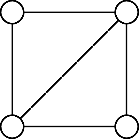
Where, is the diamond pattern, the -simplex, and are the two hypergraphs shown in Fig. 5. It turns out that simplex-reducible patterns are also cycle-reducible. Hence we can set and show that every -computable pattern is also -computable.
Lemma 5.3.
If a pattern is -computable, then it is also -computable
We can show that all the hypergraphs in can be counted in subquadratic time.
Lemma 5.4.
For any weighted colored hypergraph with edges, there is an algorithm that computes for all patterns in time .
Finally we can prove the main theorem.
See 1.1
Proof.
Let be a pattern with or less vertices. From Lemma 1.4 we have that is -computable, using Lemma 5.3 we will have that it is also -computable. Additionally, from Lemma 5.4 we have that for all hypergraphs we can compute in time. This together with Lemma 3.6 gives that we compute in time.
All the graphs in the Spasm of have also at most vertices, hence we can compute for them and use inclusion-exclusion to obtain the value of in total time .
6 Counting cycles
We adapt the two algorithms for counting weighted homomorphisms of cycles shown in [29] for computing . The first is a combinatorial algorithm that matches the complexity of detecting directed cycles combinatorially [3]. The second is a matrix multiplication based algorithm which adapts the algorithm from [53]. The complexity of this algorithm for counting is given by the value , the exact values of for are not known, but the following upper bound holds [20]:
| (2) |
Where is the matrix multiplication exponent.
Lemma 6.1.
Let be a colored weighted graph with edges. For all :
-
There is a combinatorial algorithm that computes in time .
-
There is an algorithm that computes in time .
For any we use for the fastest of the two algorithms, similar to [29]. Lemma 1.5 follows directly from Lemma 6.1 and the following equation:
| (3) |
Note that for all , hence we have subquadratic algorithms for all cycles. For and using the best known upper bound on the matrix multiplication exponent [2], we have that the matrix multiplication algorithm is faster and we get the following bounds on : , and .
References
- [1] Nesreen K. Ahmed, Jennifer Neville, Ryan A. Rossi, and Nick Duffield. Efficient graphlet counting for large networks. In Proceedings, SIAM International Conference on Data Mining (ICDM), 2015. doi:10.1109/ICDM.2015.141.
- [2] Josh Alman, Ran Duan, Virginia Vassilevska Williams, Yinzhan Xu, Zixuan Xu, and Renfei Zhou. More asymmetry yields faster matrix multiplication. In Proceedings of the 2025 Annual ACM-SIAM Symposium on Discrete Algorithms (SODA), pages 2005–2039, 2025. doi:10.1137/1.9781611978322.63.
- [3] Noga Alon, Raphael Yuster, and Uri Zwick. Finding and counting given length cycles. Algorithmica, 17(3):209–223, 1997. doi:10.1007/BF02523189.
- [4] Suman K Bera, Amit Chakrabarti, and Prantar Ghosh. Graph coloring via degeneracy in streaming and other space-conscious models. In International Colloquium on Automata, Languages and Programming, 2020. doi:10.4230/LIPIcs.ICALP.2020.11.
- [5] Suman K. Bera, Lior Gishboliner, Yevgeny Levanzov, C. Seshadhri, and Asaf Shapira. Counting subgraphs in degenerate graphs. Journal of the ACM (JACM), 69(3), 2022. doi:10.1145/3520240.
- [6] Suman K Bera, Noujan Pashanasangi, and C Seshadhri. Linear time subgraph counting, graph degeneracy, and the chasm at size six. In Proc. 11th Conference on Innovations in Theoretical Computer Science. Schloss Dagstuhl – Leibniz-Zentrum für Informatik, 2020. doi:10.4230/LIPIcs.ITCS.2020.38.
- [7] Suman K. Bera, Noujan Pashanasangi, and C. Seshadhri. Near-linear time homomorphism counting in bounded degeneracy graphs: The barrier of long induced cycles. In Proceedings of the Thirty-Second Annual ACM-SIAM Symposium on Discrete Algorithms, pages 2315–2332, 2021. doi:10.1137/1.9781611976465.138.
- [8] Suman K Bera and C Seshadhri. How the degeneracy helps for triangle counting in graph streams. In Principles of Database Systems, pages 457–467, 2020. doi:10.1145/3375395.3387665.
- [9] Umberto Bertele and Francesco Brioschi. On non-serial dynamic programming. J. Comb. Theory, Ser. A, 14(2):137–148, 1973. doi:10.1016/0097-3165(73)90016-2.
- [10] Christian Borgs, Jennifer Chayes, László Lovász, Vera T. Sós, and Katalin Vesztergombi. Counting graph homomorphisms. In Topics in discrete mathematics, pages 315–371. Springer, 2006. doi:10.1007/3-540-33700-8_18.
- [11] Marco Bressan. Faster subgraph counting in sparse graphs. In 14th International Symposium on Parameterized and Exact Computation (IPEC 2019). Schloss Dagstuhl – Leibniz-Zentrum für Informatik, 2019. doi:10.4230/LIPIcs.IPEC.2019.6.
- [12] Marco Bressan. Faster algorithms for counting subgraphs in sparse graphs. Algorithmica, 83:2578–2605, 2021. doi:10.1007/s00453-021-00811-0.
- [13] Marco Bressan, Matthias Lanzinger, and Marc Roth. The complexity of pattern counting in directed graphs, parameterised by the outdegree. In Annual ACM Symposium on the Theory of Computing, pages 542–552, 2023. doi:10.1145/3564246.3585204.
- [14] Marco Bressan and Marc Roth. Exact and approximate pattern counting in degenerate graphs: New algorithms, hardness results, and complexity dichotomies. In 2021 IEEE 62nd Annual Symposium on Foundations of Computer Science (FOCS), pages 276–285, 2022. doi:10.1109/FOCS52979.2021.00036.
- [15] Graham R Brightwell and Peter Winkler. Graph homomorphisms and phase transitions. Journal of combinatorial theory, series B, 77(2):221–262, 1999. doi:10.1006/jctb.1999.1899.
- [16] Karl Bringmann and Egor Gorbachev. A fine-grained classification of subquadratic patterns for subgraph listing and friends, 2024. doi:10.48550/arXiv.2404.04369.
- [17] Ashok K Chandra and Philip M Merlin. Optimal implementation of conjunctive queries in relational data bases. In Proc. 9th Annual ACM Symposium on the Theory of Computing, pages 77–90, 1977. doi:10.1145/800105.803397.
- [18] Norishige Chiba and Takao Nishizeki. Arboricity and subgraph listing algorithms. SIAM Journal on Computing (SICOMP), 14(1):210–223, 1985. doi:10.1137/0214017.
- [19] Radu Curticapean, Holger Dell, and Dániel Marx. Homomorphisms are a good basis for counting small subgraphs. In Proceedings of the 49th Annual ACM SIGACT Symposium on Theory of Computing, pages 210–223, 2017. doi:10.1145/3055399.3055502.
- [20] Mina Dalirrooyfard, Thuy Duong Vuong, and Virginia Vassilevska Williams. Graph pattern detection: hardness for all induced patterns and faster non-induced cycles. In Proceedings of the 51st Annual ACM SIGACT Symposium on Theory of Computing, STOC 2019, Phoenix, AZ, USA, June 23-26, 2019, pages 1167–1178, 2019. doi:10.1145/3313276.3316329.
- [21] Víctor Dalmau and Peter Jonsson. The complexity of counting homomorphisms seen from the other side. Theoretical Computer Science, 329(1-3):315–323, 2004. doi:10.1016/j.tcs.2004.08.008.
- [22] Holger Dell, Marc Roth, and Philip Wellnitz. Counting answers to existential questions. In Proc. 46th International Colloquium on Automata, Languages and Programming. Schloss Dagstuhl – Leibniz-Zentrum für Informatik, 2019. doi:10.4230/LIPIcs.ICALP.2019.113.
- [23] Josep Díaz, Maria Serna, and Dimitrios M Thilikos. Counting h-colorings of partial k-trees. Theoretical Computer Science, 281(1-2):291–309, 2002. doi:10.1016/S0304-3975(02)00017-8.
- [24] Martin Dyer and Catherine Greenhill. The complexity of counting graph homomorphisms. Random Structures & Algorithms, 17(3-4):260–289, 2000. doi:10.1002/1098-2418(200010/12)17:3/4\%3C260::AID-RSA5\%3E3.0.CO;2-W.
- [25] Martin E Dyer and David M Richerby. On the complexity of# csp. In Proc. 42nd Annual ACM Symposium on the Theory of Computing, pages 725–734, 2010. doi:10.1145/1806689.1806789.
- [26] David Eppstein. Arboricity and bipartite subgraph listing algorithms. Information processing letters, 51(4):207–211, 1994. doi:10.1016/0020-0190(94)90121-X.
- [27] Escape. https://bitbucket.org/seshadhri/escape.
- [28] Jörg Flum and Martin Grohe. The parameterized complexity of counting problems. SIAM Journal on Computing (SICOMP), 33(4):892–922, 2004. doi:10.1137/S0097539703427203.
- [29] Lior Gishboliner, Yevgeny Levanzov, Asaf Shapira, and Raphael Yuster. Counting homomorphic cycles in degenerate graphs. ACM Trans. Algorithms, 19(1), February 2023. doi:10.1145/3560820.
- [30] G. Goel and J. Gustedt. Bounded arboricity to determine the local structure of sparse graphs. In International Workshop on Graph-Theoretic Concepts in Computer Science, pages 159–167. Springer, 2006. doi:10.1007/11917496_15.
- [31] Rudolf Halin. S-functions for graphs. Journal of geometry, 8(1-2):171–186, 1976. doi:10.1007/BF01917434.
- [32] Russell Impagliazzo, Ramamohan Paturi, and Francis Zane. Which problems have strongly exponential complexity? In Proc. 39th Annual IEEE Symposium on Foundations of Computer Science, pages 653–662, 1998. doi:10.1109/SFCS.1998.743516.
- [33] Alon Itai and Michael Rodeh. Finding a minimum circuit in a graph. SIAM Journal on Computing, 7(4):413–423, 1978. doi:10.1137/0207033.
- [34] Shweta Jain and C Seshadhri. A fast and provable method for estimating clique counts using Turán’s theorem. In Proceedings, International World Wide Web Conference (WWW), pages 441–449, 2017. doi:10.1145/3038912.3052636.
- [35] Madhav Jha, C Seshadhri, and Ali Pinar. Path sampling: A fast and provable method for estimating 4-vertex subgraph counts. In Proc. 24th Proceedings, International World Wide Web Conference (WWW), pages 495–505. International World Wide Web Conferences Steering Committee, 2015. doi:10.1145/2736277.2741101.
- [36] Balagopal Komarath, Anant Kumar, Suchismita Mishra, and Aditi Sethia. Finding and Counting Patterns in Sparse Graphs. In 40th International Symposium on Theoretical Aspects of Computer Science (STACS 2023), pages 40:1–40:20, 2023. doi:10.4230/LIPIcs.STACS.2023.40.
- [37] László Lovász. Operations with structures. Acta Mathematica Academiae Scientiarum Hungarica, 18(3-4):321–328, 1967. doi:10.1007/BF02280291.
- [38] László Lovász. Large networks and graph limits, volume 60. American Mathematical Soc., 2012. URL: http://www.ams.org/bookstore-getitem/item=COLL-60.
- [39] David W Matula and Leland L Beck. Smallest-last ordering and clustering and graph coloring algorithms. Journal of the ACM (JACM), 30(3):417–427, 1983. doi:10.1145/2402.322385.
- [40] Mark Ortmann and Ulrik Brandes. Efficient orbit-aware triad and quad census in directed and undirected graphs. Applied network science, 2(1), 2017. doi:10.1007/s41109-017-0027-2.
- [41] Noujan Pashanasangi and C Seshadhri. Efficiently counting vertex orbits of all 5-vertex subgraphs, by evoke. In Proc. 13th International Conference on Web Search and Data Mining (WSDM), pages 447–455, 2020. doi:10.1145/3336191.3371773.
- [42] Ali Pinar, C Seshadhri, and Vaidyanathan Vishal. Escape: Efficiently counting all 5-vertex subgraphs. In Proceedings, International World Wide Web Conference (WWW), pages 1431–1440, 2017. doi:10.1145/3038912.3052597.
- [43] Natasa Przulj. Biological network comparison using graphlet degree distribution. Bioinformatics, 23(2):177–183, 2007. doi:10.1093/bioinformatics/btl301.
- [44] Neil Robertson and Paul D. Seymour. Graph minors. i. excluding a forest. Journal of Combinatorial Theory, Series B, 35(1):39–61, 1983. doi:10.1016/0095-8956(83)90079-5.
- [45] Neil Robertson and Paul D. Seymour. Graph minors. iii. planar tree-width. Journal of Combinatorial Theory, Series B, 36(1):49–64, 1984. doi:10.1016/0095-8956(84)90013-3.
- [46] Neil Robertson and Paul D. Seymour. Graph minors. ii. algorithmic aspects of tree-width. Journal of algorithms, 7(3):309–322, 1986. doi:10.1016/0196-6774(86)90023-4.
- [47] Marc Roth and Philip Wellnitz. Counting and finding homomorphisms is universal for parameterized complexity theory. In Proc. 31st Annual ACM-SIAM Symposium on Discrete Algorithms, pages 2161–2180, 2020. doi:10.1137/1.9781611975994.133.
- [48] C. Seshadhri. Some vignettes on subgraph counting using graph orientations. In Proceedings of the International Conference on Database Theory (ICDT), pages 3:1–3:10, 2023. doi:10.4230/LIPIcs.ICDT.2023.3.
- [49] C. Seshadhri and Srikanta Tirthapura. Scalable subgraph counting: The methods behind the madness: WWW 2019 tutorial. In Proceedings, International World Wide Web Conference (WWW), 2019. doi:10.1145/3308560.3320092.
- [50] Nino Shervashidze, S. V. N. Vishwanathan, Tobias Petri, Kurt Mehlhorn, and Karsten M. Borgwardt. Efficient graphlet kernels for large graph comparison. In AISTATS, pages 488–495, 2009. URL: http://proceedings.mlr.press/v5/shervashidze09a.html.
- [51] K. Shin, T. Eliassi-Rad, and C. Faloutsos. Patterns and anomalies in -cores of real-world graphs with applications. Knowledge and Information Systems, 54(3):677–710, 2018. doi:10.1007/s10115-017-1077-6.
- [52] George Szekeres and Herbert S Wilf. An inequality for the chromatic number of a graph. Journal of Combinatorial Theory, 4(1):1–3, 1968. doi:10.1016/S0021-9800(68)80081-X.
- [53] Raphael Yuster and Uri Zwick. Detecting short directed cycles using rectangular matrix multiplication and dynamic programming. In Proceedings of the Fifteenth Annual ACM-SIAM Symposium on Discrete Algorithms, SODA ’04, pages 254–260, 2004. URL: http://dl.acm.org/citation.cfm?id=982792.982828.