An Efficient Algorithm to Compute the Minimum Free Energy of Interacting Nucleic Acid Strands

Abstract
The information-encoding molecules RNA and DNA bind via base pairing to form an exponentially large set of secondary structures. Practitioners need algorithms to predict the most favoured structures, called minimum free energy (MFE) structures, or to compute a partition function that allows assigning a probability to any structure. MFE prediction is NP-hard in the presence pseudoknots – base pairings that violate a restricted planarity condition. However, for single-stranded unpseudoknotted structures, there are polynomial time dynamic programming algorithms. For multiple strands, the problem is significantly more complicated: Codon, Hajiaghayi and Thachuk [DNA27, 2021] proved it NP-hard for bases and strands. Dirks, Bois, Schaeffer, Winfree and Pierce [SIAM Review, 2007] gave a polynomial time partition function algorithm for multiple () strands, now widely-used, however their technique did not generalise to MFE which they left open.
We give an time algorithm for unpseudoknotted multiple () strand MFE prediction, answering the open problem from Dirks et al. The challenge lies in considering the rotational symmetry of secondary structures, a global feature not immediately amenable to local subproblem decomposition used in dynamic programming. Our proof has two main technical contributions: First, a characterisation of symmetric secondary structures implying only quadratically many need to be considered when computing the rotational symmetry penalty. Second, that bound is leveraged by a backtracking algorithm to efficiently find the MFE in an exponential space of contenders.
Keywords and phrases:
Minimum free energy, MFE, partition function, nucleic acid, DNA, RNA, secondary structure, computational complexity, algorithm analysis and design, dynamic programmingCategory:
Track A: Algorithms, Complexity and GamesCopyright and License:
2012 ACM Subject Classification:
Theory of computation Algorithm design techniques ; Theory of computation Dynamic programmingAcknowledgements:
We thank Constantine Evans for his helpful comments on the origin of the MFE rotational symmetry penalty from statistical mechanics, Mark Fornace, Niles Pierce, Dave Doty, Erik Winfree and Anne Condon for helpful comments.Funding:
Supported by Science Foundation Ireland (SFI) under grant number 20/FFP-P/8843, European Research Council (ERC) under the European Union’s Horizon 2020 research and innovation programme (grant agreement No 772766, Active-DNA project), and Funded by the European Union - European Innovation Council (EIC) and SMEs Executive Agency (EISMEA). Grant number 101115422, DISCO project. Views and opinions expressed are however those of the author(s) only and do not necessarily reflect those of the European Union, ERC, EIC, SMEs Executive Agency (EISMEA) or SFI. Neither the European Union nor the granting authority can be held responsible for them.Editors:
Keren Censor-Hillel, Fabrizio Grandoni, Joël Ouaknine, and Gabriele PuppisSeries and Publisher:
1 Introduction
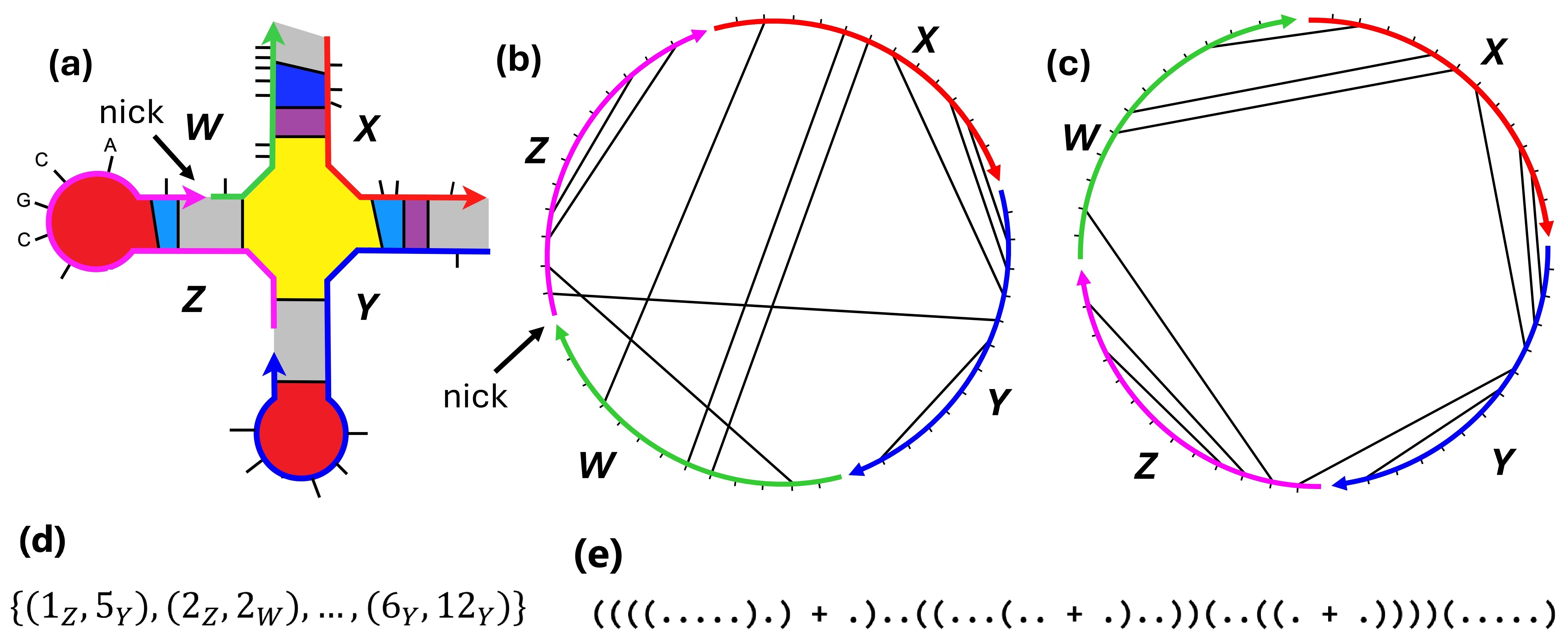
The primary structure of a DNA strand is simply a word over the alphabet , or for RNA. Bases may bond in pairs, binds to and binds to , and a set of such pairings for a strand is called a secondary structure as shown in Figure 1(a); typically each strand has exponentially many possible secondary structures. Mainly, what practitioners care about are probabilities of a given secondary structure or class of secondary structures. For that, each secondary structure has an associated, typically negative, real valued free energy , where more negative is deemed more favourable. Thus the most favourable is the secondary structure, or structures, with minimum free energy (MFE). More generally, the Boltzman distribution is a probability distribution on secondary structures at equilibrium: the probability of is , where is a normalisation factor called the partition function:
| (1) |
that is, an exponentially weighted sum of the free energies over the set of all secondary structures, where is Boltzmann’s constant and is temperature in Kelvin.111Although we use a few terms from physics/chemistry, the objects we analyse in this paper are sets of tuples (i.e. secondary structures) with straightforward mathematical definitions amenable to dynamic programming and mathematical analysis. In particular, we ignore 3D geometry–the literature has already established that simple secondary structure models nicely thread the line between having a mathematical/computational model, and being predictive for experimental conditions [10, 17, 30].
| Input type | MFE | Partition function |
|---|---|---|
| Single strand | [47, 46, 25, 24, 39]5 | [23]5 |
|
Multiple strands, bounded,
i.e. strands |
[Theorem 1] | [10]5 |
|
Multiple strands, unbounded,
i.e. strands |
APX-hard [9] | Open problem |
1.1 Related work
Decades ago, the deep relationship between secondary structures and dynamic programming algorithms was established [47, 46, 25, 24, 39, 23]. If a secondary structure can be drawn as a polymer graph without edge crossings it is called unpseudoknotted (Figure 1(c)). The earliest polynomial time algorithms were for single-stranded unpseudoknotted secondary structures, where the absence of crossings allows for planar decompositions of secondary structures suited to dynamic programming techniques.222We do not study pseudoknotted structures here, indeed most literature ignores pseudoknots for both modelling and algorithmic considerations: Energy models for pseudoknots are difficult to formulate for geometric reasons [10]. Pseudoknotted MFE prediction is NP-hard even for a single strand [1, 20, 21]. Early NP-hardness results [1, 20] used a simple energy model (no loops, only consecutive base pairs forming “stacks” contribute to free energy). Already seeing hardness results with simple energy models make it unlikely that MFE prediction problem for more realistic energy models [9] is tractable. Nevertheless, dynamic programming algorithms exist for restricted classes of pseudoknots, for both MFE [28, 37, 7, 18, 27] and partition function [11, 12]. For a single RNA/DNA strand, both MFE and partition function are computable in time5 (Table 1), using the standard nearest neighbour energy model333The standard model we use is variably called the nearest neighbour model, the Turner model, or loop energy model. Versions of the model have been implemented in software suites such as NUPACK [10, 12, 15], ViennaRNA [19] and mfold [45], for both RNA and DNA [29, 30]. that will be formally defined in Section 2.
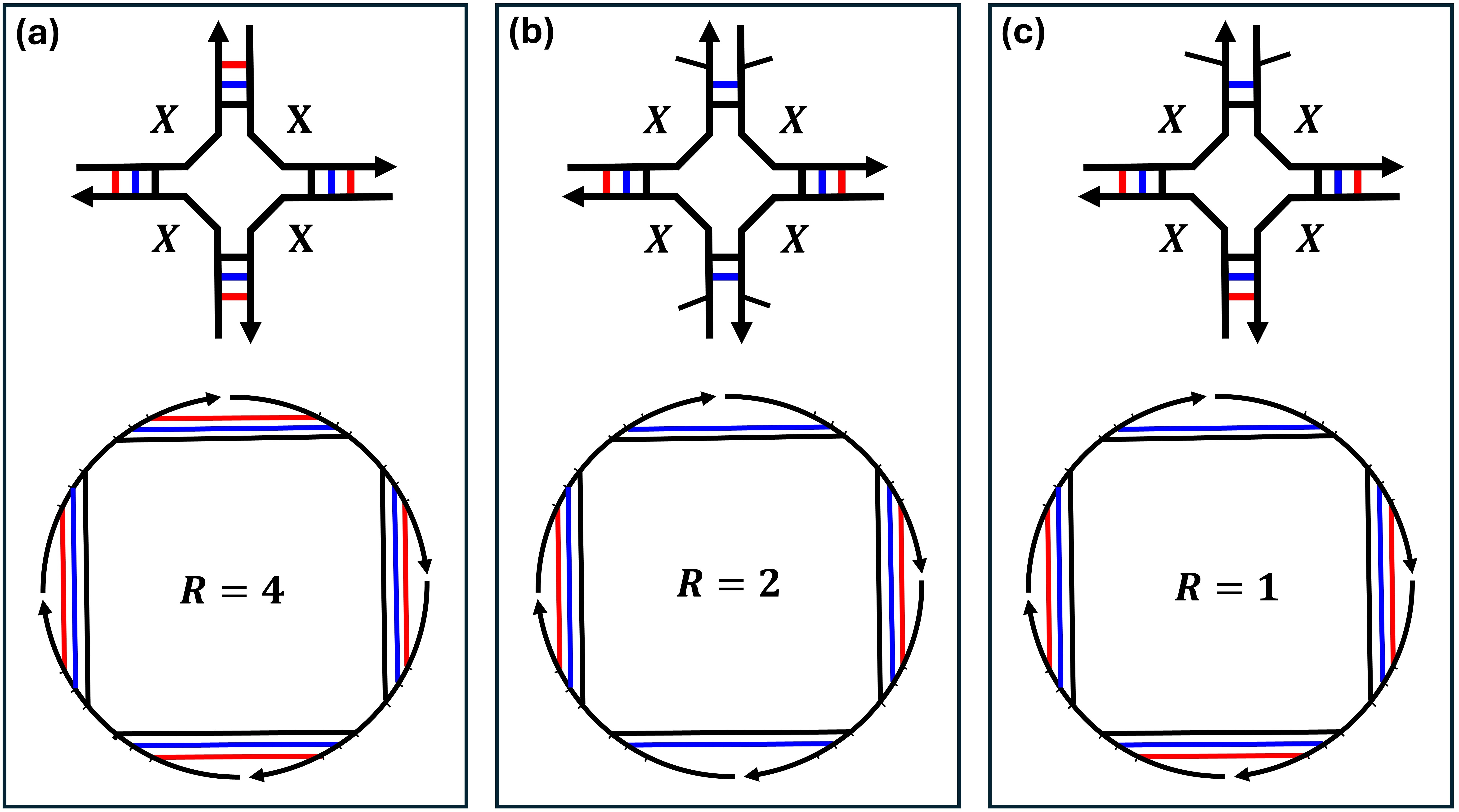
Work in DNA computing [42, 26, 35, 38, 14, 6, 32, 44], and nucleic acid nanotechnology more generally [16, 41], involves building molecular systems and structures with, to date, hundreds, and soon, thousands, of interacting strands, so there is a need for better algorithms for these multi-stranded “inverse design problems” [8, 13]. And, of course, biologists need to understand molecular structure in order to understand and predict molecular interactions. However, when there are multiple interacting strands, the situation becomes significantly more complicated than the single-stranded case for two reasons: First, for a secondary structure to be unpseudoknotted, it implies there should be at least one permutation of the strands without crossings on the polymer graph [10] (Figure 1). Second, if strand types are repeated then so-called rotational symmetries (Figure 2) arise that need to be accounted for in the model to match the underlying statistical mechanics444This fact from statistical mechanics is discussed in some papers [10, 17], although we’ve not found its full derivation in the modern nucleic-acid algorithmic literature. We leave a first-principles derivation for future work., otherwise structures may be over- or undercounted, leading to incorrect probabilities in the Boltzmann distribution, in other words: incorrect predicted free energy of a secondary structure.
For multiple strands, albeit a constant number , Dirks, Bois, Schaeffer, Winfree and Pierce [10] gave a polynomial time partition function algorithm that runs in time .555We note that in the original literature [23, 10] that established these results, the polynomial is to the power 4 due to interior loop contributions (i.e. for single-stranded and ) for multistranded). The subsequent improvement in the exponent from 4 to 3 is achieved using techniques in Dirks and Pierce (2003) [11] to handle the energy contributions of interior loops more efficiently in dynamic programming. Interestingly, Boehmer, Berkemer, Will, and Ponty [3] recently reduced the -strand parameterized running time for computing partition function and symmetry-naive MFE (i.e. ignoring rotational symmetry) from factorial, , to exponential, . In future work, it could be possible to similarly improve the factor in our MFE algorithm via this result.
In the case where the number of strands is non-constant, in particular , Codon, Hajiaghayi and Thachuk [9] showed MFE is NP-hard, and even APX-hard.666This hardness result holds whether or not rotational symmetries are accounted for in the energy model. For the second, rotational symmetry, problem, in order to compute partition function, Dirks et al. [10] found an algebraic link between the overcounting and the rotational symmetry correction problems, which allowed both to be solved simultaneously, aided by the exponential nature of the partition function. Surprisingly, that trick does not work for MFE: Since MFE prediction is minimization-based, there is no secondary structure overcounting problem in MFE prediction. In other words, unlike the case of summation-based partition function, algorithmic examination of repeated secondary structures will not change the outcome of energy minimization. Hence, the absence of the overcounting problem makes MFE prediction harder to solve, and was left open by Dirks et al. [10]. For the special case of strands, Hofacker, Reidys, and Stadler [17] gave an algorithm.
1.2 Statement of main result
We give an efficient solution to the -strand MFE problem, the first that runs in polynomial time. Our main result is stated as the following theorem, whose proof is in Section 5:
Theorem 1.
There is an time and space algorithm for the Minimum Free Energy unpseudoknotted secondary structure prediction problem, including rotational symmetry, for a set of DNA or RNA strands of total length bases.
In Section 5 we give a time-space trade-off for our result, by showing a variation of the algorithm runs in time but space.
We use the standard [10] definition of free energy (Equation 2) of multistranded unpseudoknotted secondary structures, which includes rotational symmetry, see Section 2 for formal definitions. We first give an extensive overview of the proof and paper structure, followed by future work.
1.3 Proof overview and paper structure
1.3.1 The main challenge: handling rotational symmetry
Typically, although not always, each DNA base pair that forms represents a decrease in free energy (more favourable). In a multi-stranded system, when several strands bind together the entropy of the overall system is decreased since there are now less system states due to their being less free molecules. Thus the energy model for multistranded systems includes an entropic association penalty for every extra strand, beyond the first, bound into a multistranded molecular complex [10] (typically positive, less favourable). However, statistical mechanics tells us to be careful about symmetry: with multiple identical strands in a complex it is possible that the complex is rotationally symmetric, intuitively there are several complexes, identical up to rotation of their polymer graphs (Figure 2).777Formally, we mean the permutation representing the complex is rotationally symmetric. These so-called indistinguishable complexes, in turn imply that another (positive) penalty should be applied to account for the difference in entropy between a similar, but distinguishable, complex without rotational symmetry [4, 2, 34, 15].4 Section 2 gives definitions to formalise these concepts, including: DNA, unpseudoknotted secondary structure, polymer graph, free energy including rotational symmetry (Equation 2) and MFE (Equation 3). In particular, Section 2.3 gives a group-theoretic definition of rotational symmetry, to help formalise some of the prior work.
1.3.2 General approach to find the true MFE
One obvious idea might be to find a dynamic programming algorithm that directly handles rotational symmetry. However, this approach suffers from rotational symmetry being a global property of an entire system state (secondary structure), whereas dynamic programming relies on piecing together subproblems that are individually unaware of the global context – or more precisely may be used in multiple global contexts whether symmetric or not.
Instead, our strategy is to first compute what we call the symmetry-naive MFE (snMFE) that (incorrectly) assumes all strands are distinct and thus does not compute correct free energies for rotational symmetries. We use the snMFE algorithm of Dirks et al. [10], that assumes all strands are distinct, but augmented to return extra dynamic programming matrices (Algorithm 1 in Appendix B of the full version [33]). We prove that we can use these extra matrices to help reduce the time complexity of the backtracking algorithm, hence compute the required symmetry correction to the snMFE value efficiently, as follows.
1.3.3 Polynomial upper bound: intuition for Section 3
Our goal is to show that, after running our augmentation of the known algorithm for snMFE, we have implicit access to a collection of secondary structures that are “not too far” from the true MFE – where by “not too far” we mean we have a polynomial upper bound on the number of structures to be considered by a fast backtracking algorithm that finds the true MFE structure.
First, to see how we find this polynomial bound, imagine the augmented snMFE algorithm finds that the secondary structure with snMFE is rotationally asymmetric, hence we are done, we know that the snMFE value is in fact the true MFE. Otherwise, we have a rotationally symmetric secondary structure: ideally we would like to compute its rotational symmetry degree (takes linear time in the size of the secondary structure), and then return as the true MFE, but this approach is doomed to fail since there could also be structures with lower true MFE, i.e. in the real interval .
Leveraging the two properties of being (a) unpseudoknotted and (b) rotationally symmetric, in Section 3 we define a class of cuts of a structure’s polymer graph (Figures 1 and 3) that we call pizza cuts, or, more formally, admissible symmetric backbone cuts (Definition 15). These cuts are radially symmetric, hence the name pizza cut – how one slices a pizza from disk-edge to centre. In Lemmas 14 and 24, we show that there are at most a polynomial number of pizza cuts that symmetric structures may have. We use the pizza metaphor to denote secondary structure, and pizza slice for substructure.
Then, when we do a backtracking-based search (below), through the dynamic programming matrices from the structure(s) with snMFE, to larger free energies: if we find two different symmetric pizzas, but with the same pizza cuts, we make a new pizza, by swapping a slice from one with a slice from the other. We prove that the new pizza is (a) guaranteed to be asymmetric and (b) has free energy sandwiched between the snMFE values of two symmetric structures (Lemmas 22 and 23). Hence, during the backtracking and in the worst case of reaching the polynomial upper bound exhausting the set of all admissible symmetric backbone cuts, it is guaranteed to output the true MFE structure either it was symmetric or not.
1.3.4 Backtracking to find the true MFE
It remains to show how we will do the backtracking search mentioned above. In Section 4 of the full version of this paper [33], we analyse the backtracking algorithm from Appendix C of [33], which is a polynomial time algorithm over the exponentially large set of structures “close” to the true MFE value. It scans all secondary structures within an energy level starting with the snMFE energy level, and goes on to sequentially scan higher levels in low-to-high order. The scanning process at any energy level guarantees that each secondary structure belonging to should be scanned exactly once.
The backtracking algorithm runs until one of the following conditions occurs: (1) It scans an asymmetric secondary structure , or (2) it exceeds the polynomial upper bound of the number of symmetric secondary structures (i.e. the number of distinct pizza cuts) to be scanned, or (3) the backtracking will start scanning a new energy level , where is the current best candidate for MFE (the starting value for is where is the highest degree of rotational symmetry, Definition 7). Then, based on the condition that will occur, the algorithm directly returns the true MFE, and a secondary structure which has the true MFE will also be constructed. The short proof of Theorem 1 in Section 5 ties these results together to give the final analysis of our main result. Full technical details of the backtracking algorithm are in Section 4, and Algorithm 2 in Appendix C in the full version of this work [33].
1.4 Future work
Our algorithm runs in polynomial time for the case of strands, the term coming from the fact that our algorithm, as well as the snMFE algorithm from Dirks et al. [10], is assumed to be called from an outer loop that explicitly tries all cyclic strand permutations. Can we increase the number of strands and still have a polynomial time algorithm? We know “not by much”, since the problem is NP-complete when in a simpler energy model that merely maximises the count of base pairs [9].
Our MFE algorithm exploits a polynomial upper bound, , on the number of so-called symmetric secondary structures, or distinct pizza cuts. That bound is linear in “most” cases (Lemma 26), but quadratic in one special subcase (Lemma 24) of 2-fold rotational symmetry with a central internal loop. Reducing that special case to linear would subtract one from our algorithm’s running time and space exponent.
The computational complexity of partition function for DNA/RNA strands is less well understood than MFE. Table 1 shows an open problem for partition function on multiple strands. Intuitively, it seems that partition function should be at least as hard as MFE, however that intuition is tempered by the fact that Dirks et al.’s approach found an efficient algorithm for partition function but not MFE. Nevertheless: are there settings where partition function, or problems counting numbers of structures, are #P-hard?
2 Definition of multi-stranded DNA systems and basic lemmas
Intuitively, a single DNA strand is a sequence of nucleotide bases connected by covalent bonds which together make up the backbone of , with the left end of the sequence corresponding to the end of and the right end corresponding to the end. When drawing we label the end with an arrow which also shows the strand directionality, see Figure 1. Hydrogen bonds can form between Watson-Crick base pairs, namely C–G and A–T.
Formally, a DNA strand is a word over the alphabet of DNA bases , indexed from 1 to , where denotes the length of . A base pair is a tuple such that . For any strands, we will assign to each of them a unique distinct identifier in [10]. Each base is specified by a strand identifier and a position on that strand, denotes the base of index of strand .
2.1 Connected unpseudoknotted secondary structures and polymer graphs
Definition 2 (Secondary structure ).
For any set of DNA strands, a secondary structure is a set of base pairs such that each base appears in at most one pair, i.e. if and then are all distinct.
The graph representation of a secondary structure is the graph , where is the set of bases of each strand , and , where is the set of covalent backbone bonds connecting base with base for all bases on all strands , and is the set of base pairs in . and are disjoint.
The set of circular permutations, , of strands has size [5] (e.g., for the three strands , ), e.g., the orderings , , and are the same on a circle. Next, we define a polymer graph for each , see also Figure 1.
Definition 3 (Polymer graph).
For any secondary structure , and any ordering of its strands, the polymer graph representation of , denoted , is a graph representation of , embedded in the unit disk from , where the strands are placed in succession from their to ends around the circumference of the circle in the order given by , the bases, , are spaced evenly around the circle circumference, each element of is represented by an arc on the circumference between covalently-bonded bases, and each element of is represented by a chord between two different bases.
Definition 4 (Unpseudoknotted secondary structure).
A secondary structure is unpseudoknotted if there exists at least one circular permutation such that is planar (none of the chords cross), otherwise is pseudoknotted. An example is shown in Figure 1.
Remark 5.
In the rest of the paper we use to denote the total number of bases of a secondary structure . A secondary structure is connected if the graph representation of is a connected graph. In this work, we are only interested in connected unpseudoknotted secondary structures.
2.2 Free energy of a secondary structure
In the nearest neighbour energy model [22, 30, 10], any connected unpseudoknotted secondary structure can be decomposed into different loop types [36, 30, 22]: namely hairpin loops, interior loops, exterior loops, stacks, bulges, and multiloops as shown in Figure 1. As usual, let be Boltzmann’s constant and is the temperature in Kelvin (also a constant).888All results hold if we assume these are typical values from physics, or just 1 in appropriate units. The free energy of is defined as the sum of three terms:999Throughout this paper .
| (2) |
-
the first is itself the sum of the (well-defined, empirically-obtained) free energies of ’s constituent loops [10], where the energy of each loop , is defined with respect to the free energy of the unpaired reference state.
-
is the entropic association [10] penalty applied for each of the strands added to the first strand to form a complex of strands.
-
is the rotational symmetry of the secondary structure , illustrated in Figure 2, and to be formally defined in Section 2.3. In particular, since favourable free energies are usually negative, the term corresponds to the reduction in the entropic contribution of , as any secondary structure with an -fold rotational symmetry has a corresponding -fold reduction in its distinguishable conformational space [10] as shown in Figure 2.101010This is perhaps counter-intuitive. In a follow-up expanded version of this paper we will give a full statistical mechanics explanation, which uses the symmetry penalty to offset the fact that non-symmetrical structures are overcounted from algorithmic perspective. Dynamic programming algorithms to date for multi-stranded MFE ignored this term for reasons we outline in Section 2.3.
For strands, we let be the set (usually called the ensemble) of all connected unpseudoknotted secondary structures. For any circular permutation of the strands, let be the subset of such that each connected unpseudoknotted secondary structure is representable as a crossing-free polymer graph with circular permutation .
Remark 6 (, or ).
Dirks et al. [10] showed, in their representation theorem (Theorem 2.1), that the sets , for all , form a partitioning of , which means that every connected unpseudoknotted secondary structure belongs to exactly one for some . Hence to avoid the cumbersome phrase -strand connected unpseudoknotted secondary structure with strand ordering and polymer graph we simply write , or .
Predicting the minimum free energy means finding a minimum over the ensemble . The known strategy is to deal with each partition separately, then finding their minimum:
| (3) |
2.3 Definition of multi-stranded rotational symmetry
Here, we formalise rotational symmetry. In the previous section we assigned each one of the strands a unique identifier, dealing with them as distinct strands even if two or more have the same sequence. But in most experimental settings, strands with the same sequences are indistinguishable in the sense that they behave identically with respect to relevant measurable quantities [10]. Mathematically, we say that two strands are indistinguishable if they have the same sequence. Also, two secondary structures are indistinguishable if there exists a permutation of the implied unique strand ordering (Remark 6), that maps indistinguishable strands onto each other while preserving all base pairs, otherwise, the two structures are distinct [10].
For any strands, not necessarily distinct, they consist of strand types, usually denoted by uppercase English letters 111111In contrast with some of the literature. we exclude using for strand types; to avoid any confusion between strand and base types. A multi-stranded DNA system , is a multiset of strand types with repetition numbers such that .121212It is known [31] how to efficiently reduce the circular permutation space by getting rid of circular permutations that are redundant due to indistinguishable strands, which is important to consider when computing the partition function but needed for MFE. For such a multiset we can think of each circular permutation as a string over strand types such that each strand type appears exactly times (e.g., one valid is ).
Definition 7 (Symmetry degree of a permutation).
For any circular permutation , we say is a symmetry degree of if for some , a prefix of .
For example, are the symmetry degrees of which follows from .
For any circular permutation , its maximum symmetry degree is denoted , and the corresponding repeating prefix , such that , is the fundamental component of . It can be seen that is the smallest prefix that repeats over . Indeed, is the number of cyclic permutations that map each strand to a strand of the same type. Any repeating prefix of must be a multiple of its fundamental component, see Lemma 33, Appendix A in the full version [33].
Remark 8 (Notation: ).
For any circular permutation , its augmented version gives full ordering information for each fundamental component. For example, if , then its fundamental component is , and is its augmented version, such that , means the th strand of type in the th fundamental component of .
We can visualize any ordering by representing it as a regular -gon with each of its vertices representing a fundamental component. Let ,131313Here we use algebraic cycle notation. The order of , denoted by , is the length of which is . and consider the cyclic group141414 is isomorphic to , cyclic group of order . generated by . Intuitively, is the group of all rotational motions in plane of the regular -gon that give the same -gon. We can represent as follows: , where represents rotation of the regular -gon by the angle of , where .
Now, we are ready to define the rotational symmetry of a secondary structure and a strand ordering , intuitively, the number of rotations of its polymer graph that give the same polymer graph, as shown in Figure 2.
Definition 9 (-fold rotationally symmetric structure).
A connected unpseudoknotted secondary structure and strand ordering (and thus polymer graph ) is -fold rotational symmetric, or simply rotationally symmetric, if for any base pair in the polymer graph the rotation of that base pair by multiples of is also in . More formally: , iff for all , where is the largest subgroup151515, notationally means is a subgroup of . Every subgroup of cyclic group is also cyclic. satisfying the condition, and if .
Remark 10.
In Def. 9, we restricted to be the largest subgroup so as to be aligned with the entropic reduction penalty due to symmetry that appears in Equation 2, even if from a geometric perspective any -fold rotationally symmetric secondary structure should be also -fold rotationally symmetric if divides .
3 A polynomial upper bound on a class of rotationally symmetric secondary structures
Remark 11.
In this section, we assume a global indexing of all bases from to , and use square brackets, , to denote the covalent bond connecting bases and , given that both belong to the same strand. This notation also helps to differentiate covalent bonds from base pair (hydrogen bonds) notation.
Definition 12 (-symmetric backbone cut generated by a covalent bond).
For a connected unpseudoknotted secondary structure and strand ordering , the -symmetric backbone cut generated by covalent bond is . We call a symmetric backbone cut generator. Figure 3 shows an example.
Only one covalent bond is needed to generate its corresponding -symmetric backbone cut. Also, note that this definition excludes any cut through nicks by Remark 11. Lemma 14 in the following subsection shows that the number of unique symmetric backbone cuts is linear in .
3.1 Linear upper bound on number of unique symmetric backbone cuts
The following lemma restricts us to deal with only specific and constant number of different folding rotational symmetries, and hence constant different symmetry corrections in total. The proof of this lemma is in Appendix A in the full version [33].
Lemma 13.
If is -fold rotationally symmetric secondary structure, with a specific circular permutation , then must be a divisor of .
Lemma 14 (Upper bound on unique symmetric backbone cuts).
For any connected unpseudoknotted secondary structure of strands with total bases, with a specific strand ordering , the number of unique symmetric backbone cuts is , where is the sum of divisors of .
Proof.
In general, any covalent bond is a potential candidate for a symmetric backbone cut generator. For secondary structure with bases and strands, there are covalent bonds in by excluding all nicks. We need to compute the total number of all possible symmetric backbone cuts for every possible symmetry degree . Given a specific , the number of -symmetric backbone cuts is , since for any covalent bond in a cut , we have (all bonds in that cut generate the same cut). And, hence for any two covalent bonds and , either or they are disjoint.
Because of symmetry (see Lemma 13), and divides (denoted below). Assume that are divisors of such that , and since divisors happen in pairs (), then the total number of symmetric backbone cuts is
which is since (i.e. number of strands ).
If is a connected unpseudoknotted secondary structure with ordering , you can go from any base to in two different paths around the circumference of (clockwise or anticlockwise). We define the length function to be the length of the shorter path, including both and as follows:
| (4) |
Also, is used to denote that shorter segment of length , where the direction from base to base is the same as the system strands’ direction.
3.2 How to slice a pizza (secondary structure)
We want to slice any -fold rotationally symmetric secondary structure , like pizza, to the centre of its , without intersecting any of its base pairs. First, we formalise (Definition 15) a special type of backbone cut, called an admissible -symmetric backbone cut. Then, we will prove (Lemma 16) its existence for .
Definition 15 (Admissible -symmetric backbone cut).
For any connected unpseudoknotted secondary structure with strand ordering , the -symmetric backbone cut generated by is admissible, if for all covalent bonds , is not “enclosed” by any base pair , more formally: . An example is shown in Figure 3.
Lemma 16.
For any -fold rotationally symmetric secondary structure , there exists at least one admissible -symmetric backbone cut of .
Proof.
From , select a base pair that has maximal length , at least one of and must be a covalent bond, otherwise if both were nicks, would be disconnected (a contradiction). We claim that this covalent bond, which we denote , is an admissible -symmetric backbone cut generator, otherwise there exists a base pair such that , giving a contradiction by either: (a) must contain which contradicts the maximality of , or (b) and intersect forming a pseudoknot. All covalent bonds in have the same situation because of -fold symmetry of , which implies that is an admissible -symmetric backbone cut of .
Lemma 17.
For any connected unpseudoknotted secondary structure , if there exists at least one base pair such that , then can not be -fold rotationally symmetric.
Note that any -fold rotationally symmetric secondary structure can have more than one admissible R-symmetric cut. Before defining what we mean by a pizza slice (formally, symmetric slice in Definition 19), the following lemma ensures such a slice is connected.
Lemma 18 (Pizza slicing lemma).
For any and any -fold rotationally symmetric secondary structure , let be the graph obtained from by removing the covalent bonds of admissible -symmetric backbone cut generated by any covalent bond , such that , then is disconnected and consists exactly of connected isomorphic components.
Proof.
Lemma 16 ensures the existence of at least one admissible -symmetric backbone cut of , assume it is generated by , then by Definition 12: . For any two (recall, ) “consecutive” covalent bonds in (formally: and ), we construct the “pizza slice” to be the subgraph of induced by all vertices (or bases) that belong to . Intuitively, is the slice we get after cutting at and . At the end we will have a sequence of subgraphs . Because of symmetry, all subgraphs in are isomorphic. We claim that each subgraph in is exactly one connected component, and .
For any , first we will show that is disconnected from any other with , which follows from two observations: From Lemma 17, we know that the length of and are disjoint segments by construction (via symmetry ), hence and are not connected by a covalent bond. To see that there is no base pair connecting and : assume for the sake of contradiction that such a base pair exists in , then one of the two covalent bonds or (by the definition of above), contradicting the fact that is an admissible backbone cut. Also, it follows directly that from the definition of inducing subgraphs.
We next wish to show that each slice is connected. First, there exists such that consists of connected components, because for each , is isomorphic (so if has components then all do also). Next we will show . Since is the graph obtained from the connected graph by removing covalent bonds, so there are only two cases: (a) if each of these covalent bonds is a cut edge, or bridge [40], will consist of components, contradicting the fact that number of its components must be for some , so , implying that each subgraph in consists of exactly one component. (b) The only other case is that has components (since we’ve already shown that the slices are not connected to each other), giving the lemma statement.
Definition 19 (Symmetric slice).
From the construction in Lemma 18, each of the isomorphic subgraphs (components) in is called a symmetric slice of , denoted by . Also, the loop free energy of a symmetric slice is:
| (5) |
For any -fold symmetric secondary structure , the following lemma shows the existence of a unique loop in the center of surrounded by the outer base pairs of its symmetric slices. We call it the central loop of , and denote it by . This central loop plays a crucial role in validating our slicing and swapping strategy (Lemmas 22 and 23) and determining the exact upper bound (Lemma 25) of symmetric secondary structures need to be backtracked.
Lemma 20.
For any -fold symmetric secondary structure , there exists a single loop, that we call the central loop , that is not contained in any of the symmetric slices. If then is a multiloop, if then is either a multiloop, stack, or an internal loop.
Proof.
Using our construction in Lemma 18, let be any symmetric slice, and assume a local indexing from to for the bases in the segment . Let . Intuitively, contains all outer base pairs of , we call the nesting set of as it determines how will geometrically look like (when staring at it from the centre of the pizza).
Intuitively, we construct a path as the concatenation of a segment of covalent bonds from , and then a base pair in , then more covalent bonds, then a base pair, and so on. Formally, let , then . Note that and may be substrands of length zero. Using this construction, must be a path, otherwise will be a disconnected graph contradicting Lemma 18.
Now, we will construct this central loop as follows: for simplicity of notation, let , then . If , must be a multiloop, since a multiloop is defined by being bordered by base pairs (hydrogen bonds). If , will be a multiloop if and only if (this implies there are base pairs bordering the central loop), otherwise will be an internal loop or stack. can not be external loop otherwise this will contradict the connectedness of , nor can be a bulge nor hairpin loop as either of these will contradict the symmetry of .
Because of the crucial importance of multiloops for our strategy, we highlight the multiloop energy model that is used in the standard dynamic programming algorithms. The free energy of a multiloop has the following linear form [10]:
| (6) |
where, is called the penalty for formation of the multiloop, is called the penalty for each of its base pairs that border the interior of the multiloop, and is called the penalty for each of the free bases inside the multiloop. For any -fold symmetric secondary structure , and are shared equally between the symmetric slices of , hence divides both and . So, we denote , where is the energy contribution of each symmetric slice of to the multiloop free energy, such that .
Note 21.
For any connected unpseudoknotted secondary structure of strands, we use to denote the snMFE of , in other words . It is clear that , as the symmetry correction .
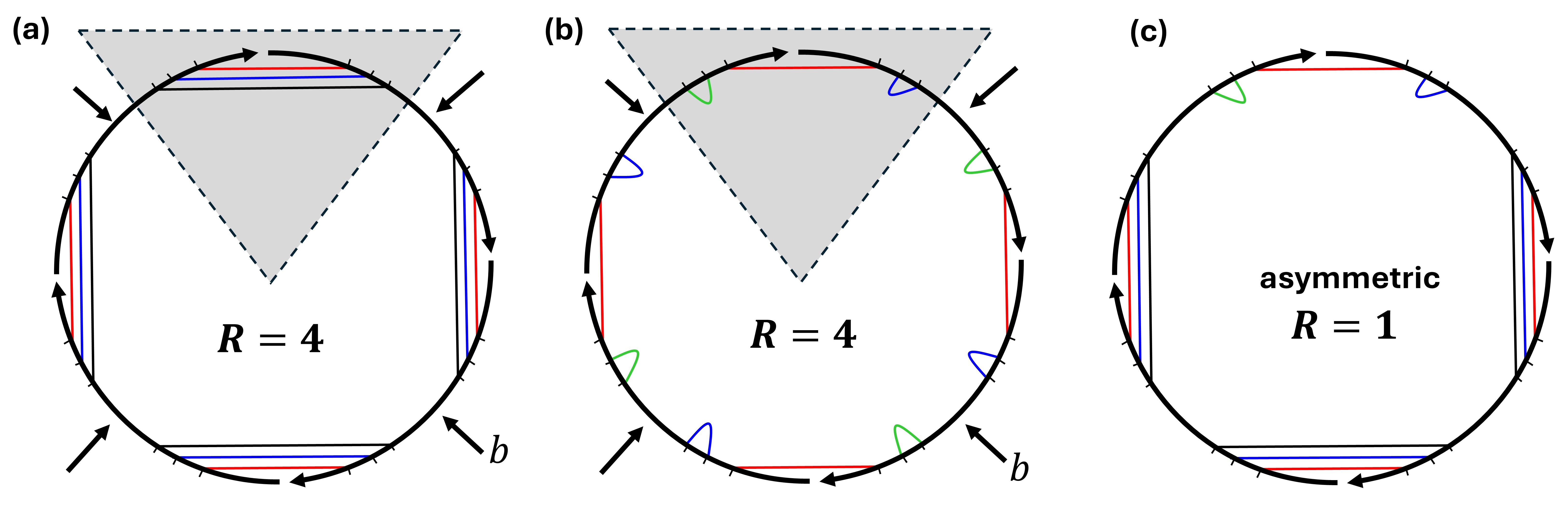
Intuitively, the following lemma lets us take two symmetric pizzas with the same admissible symmetric cut for which we know their snMFE, and swap a slice from one into the other to get a new asymmetric pizza whose true MFE lies between their snMFEs. The key intuition is that we are transforming two symmetric secondary structures into an asymmetric one.
Lemma 22 (Free-energy sandwich theorem for two -fold rotationally symmetric structures).
For any two distinct -fold rotationally symmetric secondary structures, and , of strands, such that and and and have the same R-admissible backbone cut , then there exists at least one asymmetric secondary structure , such that . Furthermore, the statement holds if and both the central loops are multiloops.
Proof.
If , from Lemma 20, there exist two unique central multiloops for and , denoted by and . Also, if , by hypothesis, and are multiloops. We prove the claim with two cases:
-
1.
:
(7) (8) (9) (10) (11) (12) We define a new secondary structure using our slicing and swapping strategy, shown in Figure 3, by removing one slice from , and adding its corresponding slice from . Lemma 18 guarantees that the new secondary structure is connected and unpseudoknotted. Furthermore, is asymmetric since . being asymmetric means that its rotational symmetry , hence we can write:
with the final step using Equation 12. Hence .
-
2.
: Following the same algebraic manipulation as Equation 7 to Equation 12, but replacing with , we get the following:
As before, we define a new connected asymmetric secondary structure , using the same slicing and swapping strategy, resulting in: .
Lemma 22 states that, if two symmetric secondary structures, having the same admissible R-symmetric backbone cut, belong to the same energy level based on the symmetry-naive MFE algorithm, ignoring symmetry entropic correction, this implies the existence of at least one asymmetric secondary structure that actually belong to the same energy level because symmetry correction for asymmetric structures is zero. If the two secondary structures belong to two different energy levels, then there exist at least one asymmetric secondary structure that actually belongs to an energy level that strictly lies between the other two energy levels.
Intuition for the case of and the central loop is not a multiloop
When , and the central loop is not a multiloop, the proof of Lemma 22 breaks. From Lemma 20, when the central loop is either a multiloop, internal loop or stack loop. The multiloop case has been handled already (Lemma 22), and the stack loop case can be subsumed into the internal loop case, since stacks are considered a special type of internal loop in the standard energy model [10]. Instead of depending on having the same admissible 2-symmetric backbone cut, we depend on sharing the same central internal loop itself, this more restricted hypothesis implies having the same admissible 2-symmetric backbone cut too, allowing us to prove Lemma 23 using a similar strategy to Lemma 22.
Lemma 23 (Free-energy sandwich theorem for two -fold rotationally symmetric structures).
For any two distinct -fold rotationally symmetric secondary structures, and , of strands, such that and both have the same central internal loop , then there exists at least one asymmetric secondary structure , such that .
Proof.
Since , then both have the same admissible 2-symmetric backbone cut as any covalent bond that belong to any side of the internal loop can be its generator.
We define a new secondary structure using our slicing and swapping strategy, shown in Figure 3, by removing one slice (half in this case) from , and adding its corresponding slice from . Note that will have also the same central internal loop . Lemma 18 guarantees that is connected and unpseudoknotted. Since is asymmetric:
Which implies that .
We now have two sandwich theorems that we can use to construct an asymmetric structure: Lemmas 22 and 23. In Section 4 we give a backtracking algorithm to search for suitable and , with the goal of applying either one of these two sandwich theorems to and . To get an overall polynomial bound for the backtracking algorithm, we wish to bound, given , how many secondary structures to scan before finding a suitable . Lemma 14 gives an upper bound on this number when applying Lemma 22. Next, Lemma 24 gives this upper bound when applying Lemma 23.
Unfortunately, the bound in Lemma 24 is larger than Lemma 14, since the energy model is more complex for internal loops than multiloops [11].
Lemma 24 (Upper bound on number of central internal loops).
For any set of strands with specific ordering , for any set of -fold rotationally symmetric secondary structures , such that each has a distinct internal central loop, the cardinality of , , where is a fundamental component of , such that , and denotes the number of bases in strand of type for all .
Proof.
Let be any set of of -fold rotationally symmetric secondary structures. Since each has a distinct internal central loop, we focus only on giving an upper bound on the maximum number of distinct internal central loops. Since , the two base pairs forming any central internal loop must be within two strands of the same type of the same order within their fundamental components (for example the strands are and ), otherwise we have a disconnected secondary structure due to the existence of nicks.
Only one of the two base pairs of any internal central loop needs to be specified explicitly, since, by symmetry, the other base pair is automatically determined. So, by considering all base pairs (including many that are irrelevant), the number of all distinct central internal loops is . Hence, . Using the two following number theoretic facts:
-
If we have two indistinguishable strands, of the same type, , of length , the maximum intra-base pairs between them happens when the sequence of is a word over or such that and or vice versa, and the same for .
-
For any integer , if , such that for all , then .
We get the following:
where , are strand types. Hence: .
3.3 Polynomial upper bound on number of symmetric secondary structures (for future backtracking)
Lemma 25.
Given an ordering of strands, for any set of distinct symmetric secondary structures such that
-
1.
for any two -fold symmetric secondary structures , where and have different admissible R-symmetric backbone cuts (we mean all possible cuts are different), and
-
2.
for any two 2-fold symmetric secondary structures , where and have different admissible R-symmetric backbone cuts (all possible cuts are different) or different central internal loops,
then , where .
Proof.
The proof is a trivial implication of Lemmas 14 and 24. (More formally: Let where is the upper bound on the number of on unique symmetric backbone cuts (Lemma 14), and is the upper bound on the number of unique central internal loops (Lemma 24). Assume for the sake of contradiction that . From the pigeon hole principle, implies repeating at least one symmetric backbone cut or a central internal loop contradicting the hypothesis about structures of .)
The (bad) quadratic bound in Lemma 24 is not that frequent: In particular, that bound only appears when and the central loop is an internal loop for both symmetric secondary structures (since this implies that the repetition number for every strand type is even, which in practice, say, for random or typical systems, may not be frequent). In particular the following lemma gives a linear bound when the repetition number of at least one strand type is odd.
Lemma 26.
For any -fold rotationally symmetric secondary structure , with ordering , such that is even, then the repetition number of each strand type must be even. Hence for any system of strands ( strand types) such that the repetition number of some strand type is odd, then , where .
Proof.
Suppose is a -fold rotationally symmetric such that is even. divides (see Lemma 13), which implies is even too. Since then such that , and this is valid only if the repetition number of each strand type is even. The linearity of follows directly if repetition number of at least one strand type is odd.
4 Backtracking to find the true MFE
The full version of this work [33] contains the technical details of the backtracking procedure used to prove Theorem 1 below, specifically see Section 4, and Algorithm 2 of Appendix C [33]. The complexity of our backtracking algorithm, is summarized in the following lemma.
Lemma 27.
The running time of the backtracking algorithm (Algorithm 2 in Appendix C in the full version of this paper [33]), for a set of DNA or RNA strands of total length bases, is , and it uses space.
5 Time and space analysis of MFE algorithm
See 1
Proof.
The snMFE algorithm of Dirks et al. runs in time and space [10]. In Algorithm 1 in Appendix B of the full version [33], we give their snMFE pseudocode but augmented with three matrices , , and , with no asymptotic change to run time but an increase to space. Also, by Lemma 27, the time complexity of our backtracking algorithm, Algorithm 2, is , and the space complexity is .
Hence after running both algorithms we get an algorithm for the MFE unpseudoknotted secondary structure prediction problem, including rotational symmetry, with space complexity .
References
- [1] Tatsuya Akutsu. Dynamic programming algorithms for RNA secondary structure prediction with pseudoknots. Discrete Applied Mathematics, 104(1-3):45–62, 2000. doi:10.1016/S0166-218X(00)00186-4.
- [2] Peter William Atkins, Julio De Paula, and James Keeler. Atkins’ physical chemistry. Oxford university press, 2023.
- [3] Kimon Boehmer, Sarah J Berkemer, Sebastian Will, and Yann Ponty. RNA triplet repeats: Improved algorithms for structure prediction and interactions. 24th International Workshop on Algorithms in Bioinformatics (WABI 2024), 2024. URL: https://hal.science/hal-04589903.
- [4] Edward Bormashenko. Entropy, information, and symmetry: Ordered is symmetrical. Entropy, 22(1):11, 2019. doi:10.3390/E22010011.
- [5] Richard A Brualdi. Introductory combinatorics. Pearson Education India, 1977.
- [6] Gourab Chatterjee, Neil Dalchau, Richard A. Muscat, Andrew Phillips, and Georg Seelig. A spatially localized architecture for fast and modular DNA computing. Nature Nanotechnology, 12(9):920–927, September 2017. doi:10.1038/nnano.2017.127.
- [7] Ho-Lin Chen, Anne Condon, and Hosna Jabbari. An algorithm for MFE prediction of kissing hairpins and 4-chains in nucleic acids. Journal of Computational Biology, 16(6):803–815, 2009. doi:10.1089/CMB.2008.0219.
- [8] Alexander Churkin, Matan Drory Retwitzer, Vladimir Reinharz, Yann Ponty, Jérôme Waldispühl, and Danny Barash. Design of RNAs: comparing programs for inverse RNA folding. Briefings in bioinformatics, 19(2):350–358, 2018. doi:10.1093/BIB/BBW120.
- [9] Anne Condon, Monir Hajiaghayi, and Chris Thachuk. Predicting minimum free energy structures of multi-stranded nucleic acid complexes is APX-hard. In 27th International Conference on DNA Computing and Molecular Programming (DNA 27). Schloss Dagstuhl – Leibniz-Zentrum für Informatik, 2021.
- [10] Robert M Dirks, Justin S Bois, Joseph M Schaeffer, Erik Winfree, and Niles A Pierce. Thermodynamic analysis of interacting nucleic acid strands. SIAM review, 49(1):65–88, 2007. doi:10.1137/060651100.
- [11] Robert M Dirks and Niles A Pierce. A partition function algorithm for nucleic acid secondary structure including pseudoknots. Journal of computational chemistry, 24(13):1664–1677, 2003. doi:10.1002/JCC.10296.
- [12] Robert M Dirks and Niles A Pierce. An algorithm for computing nucleic acid base-pairing probabilities including pseudoknots. Journal of computational chemistry, 25(10):1295–1304, 2004. doi:10.1002/JCC.20057.
- [13] David Doty and Benjamin Lee. nuad: Nucleic acid designer, March 2022. Uses, and generalises, sequence design principles from [42]. URL: https://github.com/UC-Davis-molecular-computing/nuad.
- [14] Joshua Fern and Rebecca Schulman. Design and characterization of dna strand-displacement circuits in serum-supplemented cell medium. ACS Synthetic Biology, 6(9):1774–1783, 2017. doi:10.1021/acssynbio.7b00105.
- [15] Mark E Fornace, Nicholas J Porubsky, and Niles A Pierce. A unified dynamic programming framework for the analysis of interacting nucleic acid strands: enhanced models, scalability, and speed. ACS Synthetic Biology, 9(10):2665–2678, 2020.
- [16] Cody Geary, Paul WK Rothemund, and Ebbe S Andersen. A single-stranded architecture for cotranscriptional folding of RNA nanostructures. Science, 345(6198):799–804, 2014.
- [17] Ivo L Hofacker, Christian M Reidys, and Peter F Stadler. Symmetric circular matchings and RNA folding. Discrete mathematics, 312(1):100–112, 2012. doi:10.1016/J.DISC.2011.06.004.
- [18] Hosna Jabbari, Ian Wark, Carlo Montemagno, and Sebastian Will. Knotty: efficient and accurate prediction of complex RNA pseudoknot structures. Bioinformatics, 34(22):3849–3856, 2018. doi:10.1093/BIOINFORMATICS/BTY420.
- [19] Ronny Lorenz, Stephan H Bernhart, Christian Höner zu Siederdissen, Hakim Tafer, Christoph Flamm, Peter F Stadler, and Ivo L Hofacker. ViennaRNA package 2.0. Algorithms for molecular biology, 6:1–14, 2011.
- [20] Rune B Lyngsø and Christian NS Pedersen. Pseudoknots in RNA secondary structures. In Proceedings of the fourth annual international conference on Computational molecular biology, pages 201–209, 2000.
- [21] Rune B Lyngsø and Christian NS Pedersen. RNA pseudoknot prediction in energy-based models. Journal of computational biology, 7(3-4):409–427, 2000. doi:10.1089/106652700750050862.
- [22] David H Mathews, Jeffrey Sabina, Michael Zuker, and Douglas H Turner. Expanded sequence dependence of thermodynamic parameters improves prediction of RNA secondary structure. Journal of molecular biology, 288(5):911–940, 1999.
- [23] John S McCaskill. The equilibrium partition function and base pair binding probabilities for RNA secondary structure. Biopolymers: Original Research on Biomolecules, 29(6-7):1105–1119, 1990.
- [24] Ruth Nussinov and Ann B Jacobson. Fast algorithm for predicting the secondary structure of single-stranded RNA. Proceedings of the National Academy of Sciences, 77(11):6309–6313, 1980.
- [25] Ruth Nussinov, George Pieczenik, Jerrold R Griggs, and Daniel J Kleitman. Algorithms for loop matchings. SIAM Journal on Applied mathematics, 35(1):68–82, 1978.
- [26] Lulu Qian and Erik Winfree. Scaling up digital circuit computation with DNA strand displacement cascades. Science, 332(6034):1196–1201, 2011.
- [27] Jens Reeder and Robert Giegerich. Design, implementation and evaluation of a practical pseudoknot folding algorithm based on thermodynamics. BMC bioinformatics, 5:1–12, 2004.
- [28] Elena Rivas and Sean R Eddy. A dynamic programming algorithm for RNA structure prediction including pseudoknots. Journal of molecular biology, 285(5):2053–2068, 1999.
- [29] John SantaLucia Jr. A unified view of polymer, dumbbell, and oligonucleotide DNA nearest-neighbor thermodynamics. Proceedings of the National Academy of Sciences, 95(4):1460–1465, 1998.
- [30] John SantaLucia Jr and Donald Hicks. The thermodynamics of DNA structural motifs. Annu. Rev. Biophys. Biomol. Struct., 33:415–440, 2004.
- [31] Joe Sawada. A fast algorithm to generate necklaces with fixed content. Theoretical Computer Science, 301(1-3):477–489, 2003. doi:10.1016/S0304-3975(03)00049-5.
- [32] Georg Seelig, David Soloveichik, David Yu Zhang, and Erik Winfree. Enzyme-free nucleic acid logic circuits. science, 314(5805):1585–1588, 2006.
- [33] Ahmed Shalaby and Damien Woods. An efficient algorithm to compute the minimum free energy of interacting nucleic acid strands, 2024. arXiv preprint arXiv:2407.09676. doi:10.48550/arXiv.2407.09676.
- [34] Robert J Silbey, Robert A Alberty, George A Papadantonakis, and Moungi G Bawendi. Physical chemistry. John Wiley & Sons, 2022.
- [35] Anupama J. Thubagere, Wei Li, Robert F. Johnson, Zibo Chen, Shayan Doroudi, Yae Lim Lee, Gregory Izatt, Sarah Wittman, Niranjan Srinivas, Damien Woods, Erik Winfree, and Lulu Qian. A cargo-sorting DNA robot. Science, 357(6356), 2017.
- [36] Ignacio Tinoco, Olke C Uhlenbeck, and Mark D Levine. Estimation of secondary structure in ribonucleic acids. Nature, 230(5293):362–367, 1971.
- [37] Yasuo Uemura, Aki Hasegawa, Satoshi Kobayashi, and Takashi Yokomori. Tree adjoining grammars for RNA structure prediction. Theoretical computer science, 210(2):277–303, 1999. doi:10.1016/S0304-3975(98)00090-5.
- [38] Boya Wang, Siyuan Stella Wang, Cameron Chalk, Andrew D Ellington, and David Soloveichik. Parallel molecular computation on digital data stored in DNA. Proceedings of the National Academy of Sciences, 120(37):e2217330120, 2023.
- [39] Michael S Waterman and Temple F Smith. Rapid dynamic programming algorithms for RNA secondary structure. Advances in Applied Mathematics, 7(4):455–464, 1986.
- [40] Douglas Brent West et al. Introduction to graph theory, volume 2. Prentice hall Upper Saddle River, 2001.
- [41] Sungwook Woo and Paul WK Rothemund. Programmable molecular recognition based on the geometry of DNA nanostructures. Nature chemistry, 3(8):620, 2011.
- [42] Damien Woods, David Doty, Cameron Myhrvold, Joy Hui, Felix Zhou, Peng Yin, and Erik Winfree. Diverse and robust molecular algorithms using reprogrammable DNA self-assembly. Nature, 567(7748):366–372, 2019. doi:10.1038/S41586-019-1014-9.
- [43] Joseph N Zadeh, Conrad D Steenberg, Justin S Bois, Brian R Wolfe, Marshall B Pierce, Asif R Khan, Robert M Dirks, and Niles A Pierce. Nupack: Analysis and design of nucleic acid systems. Journal of computational chemistry, 32(1):170–173, 2011. doi:10.1002/JCC.21596.
- [44] David Yu Zhang and Georg Seelig. Dynamic DNA nanotechnology using strand-displacement reactions. Nature chemistry, 3(2):103–113, 2011.
- [45] Michael Zuker. Mfold web server for nucleic acid folding and hybridization prediction. Nucleic acids research, 31(13):3406–3415, 2003. doi:10.1093/NAR/GKG595.
- [46] Michael Zuker and David Sankoff. RNA secondary structures and their prediction. Bulletin of mathematical biology, 46:591–621, 1984.
- [47] Michael Zuker and Patrick Stiegler. Optimal computer folding of large RNA sequences using thermodynamics and auxiliary information. Nucleic acids research, 9(1):133–148, 1981. doi:10.1093/NAR/9.1.133.