Faster Construction of a Planar Distance Oracle with Query Time

Abstract
We show how to preprocess a weighted undirected -vertex planar graph in time, such that the distance between any pair of vertices can then be reported in time. This improves the previous preprocessing time [JACM’23].
Our main technical contribution is a near optimal construction of additively weighted Voronoi diagrams in undirected planar graphs. Namely, given a planar graph and a face , we show that one can preprocess in time such that given any weight assignment to the vertices of one can construct the additively weighted Voronoi diagram of in near optimal time. This improves the construction time of [JACM’23].
Keywords and phrases:
Distance Oracle, Planar Graph, Construction TimeCategory:
Track A: Algorithms, Complexity and GamesCopyright and License:
2012 ACM Subject Classification:
Theory of computation Data structures design and analysisFunding:
Israel Science Foundation grant 810/21.Editors:
Keren Censor-Hillel, Fabrizio Grandoni, Joël Ouaknine, and Gabriele PuppisSeries and Publisher:
1 Introduction
In this paper we investigate the following question: How fast can you preprocess a planar graph so that subsequent distance queries can be answered in near-optimal time? Imagine you could do the preprocessing in near-optimal time. This would be truly remarkable, since it would allow us to efficiently convert between standard graph representations, which support quick local (e.g., adjacency) queries, into a representation that supports quick non-local distance queries. In a sense, this can be thought of as an analogue for distances of the Fast Fourier Transform (which converts in time between the time domain and the frequency domain). Such a tool would allow us to develop algorithms for planar graphs that can access any pairwise distance in the graph essentially for free! Unfortunately, we are still far from obtaining preprocessing time. The fastest preprocessing time is [9]. We make a step in this direction by improving the preprocessing time to in weighted undirected planar graphs.
Formally, a distance oracle is a data structure that can report the distance between any two vertices and in a graph . Distance oracles for planar graphs have been studied extensively in the past three decades both in the exact [32, 9, 19, 1, 15, 13, 17, 26, 40, 38, 4, 36, 14, 21, 10] and in the approximate [39, 23, 24, 25, 22, 41, 8, 29] settings. In the approximate setting, Thorup [39] presented a near-optimal oracle that returns -approximate distances (for any constant ) in time and requires space and construction time (see also [25, 23, 24, 22, 41, 8, 29] for polylogarithmic improvements). Is it possible that the same near-optimal bounds can be achieved without resorting to approximation? We next review the rich history of exact oracles in planar graphs.
The history of exact planar distance oracles.
Let and denote the query-time and the space of an oracle, respectively. The early planar distance oracles [1, 15, 13] were based solely on planar separators [31, 33, 18] and achieved a tradeoff of for , and for . In [17], Fakcharoenphol and Rao introduced the use of Monge matrices to distance oracles, and devised an oracle with space and query time. By combining their ideas with Klein’s [25, 6] multiple source shortest path (MSSP) data structure, Mozes and Sommer [36] obtained the tradeoff for nearly the full range . Other works [40, 38, 36, 19] focused on achieving strictly optimal query-time or strictly optimal space. Namely, Wulff-Nilsen’s work [40] gives optimal queries with weakly subquadratic space, whereas Nussbaum [38] and Mozes and Sommer’s [36] oracles give optimal space with query-time. Except for [40], all of the above oracles can be constructed in time. However, none of them provides polylogarithmic query-time using truly subquadratic space.
In FOCS 2017, Cohen-Addad, Dahlgaard, and Wulff-Nilsen [14] (inspired by Cabello’s [5] breakthrough use of Voronoi diagrams for computing the diameter of planar graphs) realized that Voronoi diagrams, when applied to regions of an -division, can be used to break the barrier mentioned above. In particular, they presented the first oracle with query-time and truly subquadratic space, or more generally, the tradeoff for any . This came at the cost of increasing the preprocessing time from to , which was subsequently improved to match the space bound [20]. In SODA 2018, Gawrychowski, Mozes, Weimann, and Wulff-Nilsen [21] improved the space and preprocessing time to with query-time (and the tradeoff to for ) by defining a dual representation of Voronoi diagrams and developing an efficient point-location mechanism on top of it. In STOC 2019, Charalampopoulos, Gawrychowski, Mozes, and Weimann [10] observed that the same point-location mechanism can be used on the Voronoi diagram for the complement of regions in the -division. This observation alone suffices to improve the oracle size to (while maintaining query-time). By combining this with a sophisticated recursion (where a query at recursion level reduces to queries at level ) they further obtained an oracle of size and query-time . Finally, in SODA 2021, Long and Pettie [32] showed how much of the point-location work can be done without recursion, and that only two (rather than ) recursive calls suffice. This led to the state of the art oracle, requiring space and query-time or space and query-time.111A journal version containing all the above Voronoi-based oracles was published in JACM in 2023 [9].
In terms of space and query time, these latter Voronoi-based oracles are almost optimal. However, their construction time is , and improving it is mentioned in [9] as an important open problem. The bottleneck behind this bound is the time for constructing Voronoi diagrams as we next explain.
Point-location in Voronoi diagrams.
Let be a planar graph, and let be a face of . The vertices of are called the sites of the Voronoi diagram, and each site has a weight associated with it. The distance between a site and a vertex , denoted by is defined as plus the length of the -to- shortest path in . The additively weighted Voronoi diagram is a partition of ’s vertices into pairwise disjoint sets, one set for each site . The set , called the Voronoi cell of , contains all vertices in that are closer (w.r.t. ) to than to any other site (we assume that distances are unique to avoid the need to handle ties222This assumption can be achieved in time. With high probability using [34, 37], or deterministically using [16].). A point-location query asks for the site whose Voronoi cell contains . There exists a dual representation of . The size of this representation is , and together with an MSSP data structure it supports point-location queries in time.
Our results and techniques.
In [9], it was shown that given the MSSP of a graph (piece) , a face of , and additive weights to the vertices of , the Voronoi diagram can be constructed in time. In this paper, we show (see Theorem 15) how to construct it in near-optimal time when the graph is undirected. As discussed below, this leads to a static distance oracle of space , construction time , and query-time . In addition, it implies a dynamic distance oracle that supports -time distance queries from a single-source , and -time updates consisting of edge insertions, edge deletions, and changing the source . The dynamic distance oracle is obtained by simply plugging our construction into the oracle of Charalampopoulos and Karczmarz [12] (thus improving its update time from to ). We note that the current best all-pairs dynamic oracle by Fakcharoenphol and Rao [17] has update time and query time. Therefore, in undirected graphs, our new oracle achieves the same bounds but has the benefit that, between source changes, the query takes only time.
Our construction is inspired by Charalampopoulos, Gawrychowski, Mozes, and Weimann who showed in ICALP 2021 [11] that near-optimal construction time is possible for the special case when the planar graph is an alignment graph of two strings. The alignment graph is an acyclic grid graph of constant degree. More importantly, shortest paths in this graph are monotone, in the sense that they only go right or down along the grid. This makes the Voronoi diagram of every piece much more structured. In particular, one can find the trichromatic vertices of (i.e., the faces of whose vertices belong to three different Voronoi cells) by recursively zooming in on them using cycle separators; The intersection of a cycle separator with each Voronoi cell consists of at most two contiguous intervals of the cycle separator. This partition induced by these intervals can be found with a binary search approach, whose complexity (up to a logarithmic factor) is linear in the number of trichromatic vertices enclosed by the cycle. From the partition it is easy to deduce whether a trichromatic vertex of is enclosed by the cycle separator, and infer whether we should recurse on each side of the separator. In this paper we extend this binary search approach to general undirected planar graphs.
At a first glance, such an extension seems impossible as the intersection of cycle separators and Voronoi cells might be very fragmented, even when there are only three sites. To overcome this, we use shortest path separators. Such separators have been widely used in essentially all approximate distance oracles for planar graphs, but also in exact algorithms (e.g., [7, 3, 28, 35]). These cycle separators may contain edges (rather than ), but consist of two shortest paths , so that, because the graph is undirected, any other shortest path can intersect each of at most once. In our context, this implies a monotonicity property when we restrict our attention to shortest paths that enter the cycle separator only from the left or only from the right. If we only allow paths to enter from one side, say the left, then the intersection of each Voronoi cell (with distances now defined under this restriction) with is a single contiguous interval.
To better explain the difficulties with this approach and how we overcome them, let us first define some terminology. We say that vertex prefers a site if belongs to (defined without any restrictions). We say that left-prefers a site if belongs to under the restriction that paths are only allowed to enter from the left. Repeating the above discussion using this terminology, the partition induced by the prefers relation may be very fragmented, but the partition induced by the left-prefers relation is not fragmented. There are two immediate problems with working with the partition induced by left-preference (or right-preference). First, we are interested in constructing the Voronoi diagram without any restrictions, and second, we do not know how to efficiently compute shortest paths under restrictions on the direction in which they enter .
To address the first difficulty we show that one can infer which sides of the cycle separator contain a trichromatic vertex of the Voronoi diagram (without restrictions) by inspecting the endpoints of the intervals of the two partitions - the one with respect to left-preference and the one with respect to right-preference. This is shown in Section 4. We also show, by adapting the divide-and-conquer construction algorithm of [20], how to reduce the problem of computing a Voronoi diagram with many sites to the problem of computing the trichromatic vertex of a Voronoi diagram with only three sites. This is explained in Section 5.
Overcoming the second difficulty is the heart of our technical contribution. We know how to efficiently determine, by enhancing the standard MSSP data structure, whether the true shortest path from a site to a vertex enters from the right or from the left. However, we do not know how to efficiently report the shortest path from to that enters from the other side (because that path is not the overall shortest path from to ). We observe that we can work with relaxed preferences. If prefers (without restrictions on left/right), then: (1) we might as well say that both right-prefers and left-prefers (because either way this will point us to ), and (2) if the shortest path from to enters from the right, we do not really care what the left preference of is, so we might as well say that left-prefers for any site . In Section 3 we describe how to compute a partition with respect to such a relaxed notion of left-preference and right-preference. The exact details are a bit more complicated than described here. In particular we use the term like rather than prefer to express that the preference is more loose.
Constructing a partition with relaxed preferences turns out to be more complicated than with strict preferences. One challenge comes from the fact that with relaxed preferences making progress in a binary search procedure is problematic. This is because a vertex of no longer has a unique left-preferred site . In fact, when working with relaxed preferences, a vertex may equally like all sites. Thus, we need to have some way to recognize a “winner” site with respect to a vertex that does not have a unique preference. Another challenge we encounter is what we call swirly paths - when the -to- path goes around before entering . Swirly paths make the realizations of many of the arguments outlined here more complicated. The structure of the shortest paths that allows us to make progress in the binary search procedure is different and more complicated in the presence of swirly paths. Moreover, we do not always know how to efficiently identify whether a shortest path is swirly or not. To simplify the presentation we first explain how to obtain a partition with respect to relaxed preferences when there are no swirly paths. In the full version of the paper [2] we describe how to handle swirly paths.
We believe that our result is a promising step toward exact oracles that simultaneously have optimal space, query-time and preprocessing time. One way to achieve this would be to be able to find a way to use recursion to obtain the functionality of our enhanced MSSP data structure without actually computing it over and over in large regions of the graph, in a similar manner to the way this issue was avoided for the standard MSSP in [9]). This seems to be the only significant obstacle preventing us from pushing our new ideas all the way through, and obtaining an almost optimal construction time for undirected planar graphs.
2 Preliminaries
Representation of Voronoi diagrams.
With a standard transformation (without increasing the size of asymptotically) we can guarantee that each vertex of has constant degree and that is triangulated. Consider a subgraph (called a piece) of whose boundary vertices (vertices incident to edges in ) lie on a single face of . Note that is the only face of that is not a triangle. The vertices of , assigned with weights , are the sites of the Voronoi diagram of . There is a dual representation of VD as a tree with vertices (see Figure 1): Let be the planar dual of . Consider the subgraph of consisting of the duals of edges of such that and are in different Voronoi cells. In this subgraph, we repeatedly contract edges incident to degree-2 vertices. The remaining vertices (edges) are called Voronoi vertices (edges). A Voronoi vertex is dual to a face whose three vertices belong to three different Voronoi cells. We call such a face (and its corresponding dual vertex) trichromatic. Finally, we define to be the tree obtained from the subgraph by replacing the node by multiple copies, one for each edge incident to . The complexity (i.e., the number of vertices and edges) of is . For example, in a VD of just two sites and , there are no trichromatic faces. In this case, is just a single edge corresponding to an -cut or equivalently to a cycle in the dual graph. We call this cycle the -bisector and denote it by . Note that a trichromatic vertex is a meeting point of three bisectors. Another important example is a VD of three sites (we call this a trichromatic VD). Such a VD has at most one trichromatic face (in addition to face itself).
Using point-location for distance oracles.
To see why point-location on Voronoi diagrams is useful for distance oracles, we describe here the -space -query oracle of [10] that we will be using. It begins with an -division of the graph . This is a partition of into subgraphs (called pieces) such that every piece contains vertices and boundary vertices (vertices shared by more than one piece). An -division can be computed in time [27] with the additional property that the boundary vertices of every piece lie on a constant number of faces of the piece (called holes). To simplify the presentation, we assume that lies on a single hole (in general, we apply the same reasoning to each hole separately, and return the minimum distance found among the holes). The oracle consists of the following for each piece of the -division:
-
1.
The space, construction time, query-time distance oracle of [21] on the graph . In total, these require space and construction time.
-
2.
Two MSSP data structures [25], one for and one for , both with sources . The MSSP for requires space , and the MSSP for requires space . Using these MSSPs, we can then query in time the -to- distance for any and . The total space and construction time of these MSSPs is , since there are pieces.
-
3.
For each vertex of , compute the Voronoi diagram (resp. ) for (resp. ) with sites and additive weights the distances from to these vertices in (the additive weights are computed in time using [17]). Each Voronoi diagram can be represented in space [21] and can be constructed in time [10]. Hence, all Voronoi diagrams require space and construction time.
To query a -to- distance, let be the piece that contains . If then the -to- path must cross . We perform a point-location query for in in time [21]. If then we return the -to- distance (from the precomputed additive weight) plus the -to- distance (from the MSSP of ). Otherwise, and we return the minimum of two options: (1) The shortest -to- path crosses . This is similar to the previous case except that the point-location query for is done in . (2) The shortest -to- path does not cross (i.e., the path lies entirely within ). We retrieve this distance by querying the distance oracle stored for .
By choosing we get an oracle of space and query-time . The construction time however is . Notice that the only bottleneck preventing construction time is the construction of the Voronoi diagrams.
Shortest path separators.
A shortest path separator is a balanced cycle separator consisting of two shortest paths and (emanating at the same vertex) plus a single edge. A complete recursive decomposition tree of using shortest path separators can be obtained in linear time [30].
An arc emanates (enters) left of a simple path if there exist two arcs , in , such that () is the head of and the tail of , and appears between and in the clockwise order of arcs incident to . Otherwise, emanates (enters) right of . Notice that this is not defined for the endpoints of , however, in the context in which we will use it, we will always extend so that its original endpoints will become internal. Specifically, consider a shortest path separator composed of an -to- path , an -to- path , and an edge . Then, we will extend on one side with and on the other side with the vertex following on . A symmetric extension will be done for .
3 Efficient Computation of a Relaxed Partition
In this section we define a relaxed partition, and show how to compute it in time.
3.1 Definitions and data structures
In our settings, let denote the face, and let denote a subset of vertices (sites) of (for the most part, we will use in order to find trichromatic faces, see Section 4). We say that vertex prefers a site if belongs to . It is natural to partition the vertices of according to the site in that they prefer. In the case of the alignment graph of [11], each part in this partition is a contiguous interval of . In general planar graphs however, this is not the case, and the parts can be very fragmented.
We observe that the partition would induce contiguous intervals if we only consider shortest paths that are allowed to enter from the right (or only from the left). In that case we can say that a vertex right-prefers (left-prefers) . We know how to determine efficiently whether the true shortest path from a site to a vertex enters from the right or from the left. But the problem is that then we do not know how to efficiently report the shortest path from to that enters from the other side (because it is not the overall shortest path from to ).
To overcome this issue we observe that we can work with relaxed preferences, which we call like. If prefers (without restrictions on left/right), then we might as well say that both right-likes and left-likes (because either way this will point us to ). Similarly, if prefers (again, without restrictions on left/right) then if the shortest path from to enters from the right, we do not really care what the left like of is (since in this case shortest paths entering from the left are just irrelevant), so we may as well say that left-likes for any site .
Recall that the endpoints of are and . We denote by and the sites of such that and . In practice we will use the left-like (and symmetrically the right-like) relation with respect to a subset of sites. If the true site in that prefers (without restrictions on left/right) is not one of the sites in then we may as well say that both left-likes and right-likes all sites in because eventually they will have no effect on the true answer.
The following definition formalizes the above discussion.
Definition 1 (-like).
Let be an -to- shortest path, let be a cyclic subsequence of a face , and let be a subsequence of . Let (resp. ) be the site such that (resp. ). A vertex that belongs to the Voronoi cell is said to -like if at least one of the following holds: (1) , (2) the shortest path from to enters from the right, or (3) .
This notion of -like, induces a relaxed partition of , in which the parts do form contiguous intervals along . The relaxed partition has the property that for every if and reaches from some (left or right) then in the -relaxed partition is in the part of corresponding to site . In other words, together, the and -relaxed partitions assign to each vertex of at most two sites in , and it is guaranteed that one of these two sites is the true site of .
Definition 2 (Relaxed Partition).
Let be a shortest path, and let and be cyclic subsequences of a face with , denoted by and .
A relaxed -partition of w.r.t. is a partition of into disjoint subpaths such that every is a vertex that -likes .
The definitions of -like and of an -relaxed partition are symmetric. The main part of our algorithm is dedicated to finding a relaxed partition. First, in Section 3.3 we will show how to find a relaxed partition of w.r.t. consisting of only two sites. Then, in Section 3.4, we explain how to obtain a relaxed partition of w.r.t. by combining the relaxed partitions of pairs of sites in .
For two vertices we denote the shortest path in between and as . For a site we denote by the set of vertices such that enters from the left.
The following lemma describes a data structure that will later (Lemma 4) allow to find an -partition of . A similar proof finds an -partition.
Lemma 3 (Enhanced MSSP data structure).
Given a planar graph , a face and a recursive decomposition of , one can construct in time a data structure supporting the following queries, each in time. For any source , shortest path , and vertex :
-
1.
- return the distance between and in .
-
2.
- return whether enters from left or right.
-
3.
for - return the number of vertices on .
-
4.
for - return the ’th vertex of .
-
5.
- return the ancestor of that is in depth in the shortest paths tree of .
Lemma 4.
Given , , and , together with their enhanced MSSP, and a shortest path , one can compute an -partition of , in time.
3.2 Setup of the query
Recall that the endpoints of are and , and that and are the sites of such that and . Notice that it is straightforward to find and in time by explicitly checking the distance from each of the sites in to and to using the enhanced MSSP. We denote and . We assume , since the case is a degenerated case.333 If one can think of the graph obtained by making an incision along , which allows us to think of as being split into two vertices, where one is the site of and the other is the site of , see also Remark 12. We also assume that , since otherwise we find a partition for , and then add the intervals of the sites in , using a binary search along . The sites and partition the face into two intervals which we denote by and . In addition, let and . The following lemma (see proof in the full version of the paper [2]) states that when computing the -partition, we can ignore every . Thus, every time we consider a partition with respect to some , we consider the vertices of from the closest vertex to to the closest vertex to (on ). In addition, the partition is always such that the order of the parts corresponding to vertices of is from the one containing to the one containing .
Lemma 5.
Every -partition is an -partition.
Remark 6.
When considering a partition of with respect to a set , the parts of in our partition are chosen so that they are consistent with the order of the vertices in . For example, the first part, corresponds to the vertex of closest to , contains (unless it is empty) and the part of the vertex closest to , contains (unless it is empty).
Trimming .
By definition and for every we also have . Therefore, w.l.o.g., we assume that contains only the vertex , since all the vertices of are known to belong to . Similarly, we assume that .
Swirly paths.
For vertices and , we say that is a swirly path if and crosses or . Moreover, a path is called -swirly (resp. -swirly) if the first path it crosses among and is (resp. ).
Swirly paths complicate life. We shall first (in Section 3.3) explain how to obtain an -partition when and there are no swirly paths. We consider the general case (with ) where there are swirly paths in the full version of the paper [2]. Finally, in Section 3.4 we will show how to obtain an -partition of , removing the restriction to two vertices and proving Lemma 4.
3.3 Partition with respect to two sites
In this subsection we show how to compute an -partition when . We start with a special case, where we consider a subpath of that is not involved in any swirly paths. Later, in Lemma 11 we introduce the algorithm for computing an -partition when .
Lemma 7.
Let be two sites such that is closer to on than . Let be a subpath of with being closer to than , such that for every and the path is non-swirly. One can compute in time an -partition of into such that and , unless the partition is trivial.
The proof of Lemma 7 consists of several steps. We first introduce the notion of winning, and show (Claim 8) that it is a monotone property of vertices of . We will then use this monotonicity to perform binary search. For a vertex we say that wins at if there exists an -to- non-swirly path that enters from the left and . We define winning at symmetrically.
To avoid clutter we assume , otherwise one just has to change in the following proofs to and to the endpoints of .
Claim 8.
Let such that wins at . Then, every is a vertex that -likes . Symmetrically, if wins at , then every is a vertex that -likes .
Proof.
We prove the first claim, the proof of the symmetric claim is similar. Since wins at , there exists an -to- non-swirly path that enters from the left and . Let . Assume by contradiction that is a vertex that does not -like . Then must enter from the left and . Hence, for any we have . Thus, . Similarly, for any we have . Hence, .
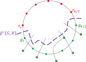
Consider the cycle composed of ,, and the Jordan curve connecting and embedded in the face . See Figure 2 (left). Notice that has no self-crossing since does not cross as is a non-swirly path. We think of as an oriented cycle whose orientation is consistent with that of (recall that the orientation of is from to ) so as to define left and right properly (i.e., define what is left and right w.r.t. ). Observe that is on the right side of . Since intersects , but does not intersect nor , it must be that intersects only among the parts of . Since is on the right side of , enters from the right, a contradiction.
Having proved that the winning property is sufficient to perform a binary search to obtain a partition of , we next show how to find a pair (where and ) such that is a winner at . We distinguish two scenarios that are handled differently (Claims 9 and 10). Later we will put it all together and show how to make this into an efficient binary search procedure.
Claim 9.
Let and be vertices such that and . If is closer on to than then there is an -time algorithm that outputs and such that wins at .
Proof.
For every , we check if enters from the left and whether is smaller than the distance of the other site to . We return a pair satisfying the claim. This takes time using the enhanced MSSP data structure of Lemma 3.
It remains to prove that at least one such pair exists. Assume by contradiction that no such pair exists. In particular, since enters from the left, it must be the case that . Moreover, must enter from the right (otherwise is a valid pair). Similarly, since enters from the left we have .
We will show that enters from the left, implying that is a valid pair, contradicting our assumption. Consider the (non self crossing) cycle . We think of as an oriented cycle whose orientation is consistent with that of so as to define left and right properly, see Figure 2 (right).
Let be the first vertex of that belongs to . Note that exists since . Since is on the left side of , enters from the left at . We will show that , which means that either (i) or (ii) . To see that notice that every satisfies and every satisfies . If (i) then enters from the left, as it enters from the left at . If (ii) then , meaning that enters from the left. To conclude, in both cases enters from the left, which contradicts our assumption.
Claim 10.
Let and be vertices such that and . If is closer on to than then there is an -time algorithm that outputs and such that wins at .
Proof.
For every we check if enters from the left and whether is smaller than the distance of the other site to . If such a pair is found, we return this pair. Otherwise, it must be that: (1) , (2) enters from the right, (3) , and (4) enters from the right.
Consider the cycle composed of , , and the Jordan curve connecting and embedded in the face . We first claim that all edges entering from the left are on the left side of . To see this, consider making an incision along (duplicating its vertices and edges). Since both and do not cross and enter from the right, they both use the right copy of , and do not intersect the left copy of . Hence, the left copy of , and hence also all edges entering from the left, are on the left side of .
The path does not intersect (since the former enters from the left and the latter enters from the right). Moreover, by uniqueness of shortest paths, does not cross nor . Thus, does not cross . Symmetrically, does not cross . Since both and start on , do not cross and enter from the left, they must be on the left side of .
Since , and it must be that . Hence, in the counterclockwise cyclic order of the vertices appear as . Therefore, the paths and form a cross configuration and must cross each other, such that crosses from left to right.
For simplicity, we assume that contains a single vertex . In the general case, it may be a contiguous subpath and the proof is similar. Our goal now is to determine whether is closer to or to . We emphasize that the algorithm does not find itself at any time.
Consider the path and notice that and . Since is a shortest path, it must be that for some vertex we have that all vertices in are closer to than to and all vertices in are closer to than to . Using queries of the enhanced MSSP (in time per query), the algorithm binary-searches for , checking at every step which of and is closer to the queried vertex. After finding , the algorithm uses enhanced MSSP to check whether appears to the right, to the left, on in the shortest path tree rooted at . We note that cannot be a descendant of in the tree of , since every vertex on is closer to than to , while is closer to than to . If is on then is closer to than to .
We will show that if is to the right of in the tree of then is closer to than to . Consider the cycle obtained by concatenating and the Jordan curve connecting and embedded in the face . We consider to be oriented from to . Notice that does not cross since and cross each other only once. Recall that is to the left of , and therefore to the left of . Additionally recall is to the right of , and therefore to the right of . Consider the first vertex of which is not on . Since is to the right of , it holds that is to the right of . Moreover is strictly to the right of . This is because is disjoint from by uniqueness of shortest paths, and is disjoint from since is closer to and is closer to . Thus, is disjoint from , and therefore is to the right of and therefore and this means is closer to than to by definition of . A similar argument shows that if is to the left of in the shortest paths tree of , then is closer to than to .
Thus, the algorithm deduces whether is closer to or to . If is closer to , the algorithm reports that wins at . This is because the path enters from the left and . Moreover, is a concatenation of subpaths of two non-swirly paths from vertices on , and therefore is a non-swirly path. Similarly, if is closer to , the algorithm reports that wins at . This is because the path enters from the left and , and is a non-swirly path.
Finally, the running time of the algorithm is indeed , since all distance queries, and directions can be answered in time per query by the enhanced MSSP of Lemma 3 and the binary search of increases the running time only by an additional factor.
Using Claims 8, 9, and 10 we introduce a recursive binary search partition algorithm, completing the proof of Lemma 7. In each recursive step, the algorithm works on a subpath , and returns a partition of into a (possibly empty) prefix and a (possibly empty) suffix such that every is a vertex that -likes (for ).
When working on , the algorithm starts by finding a “left median” vertex of in . Formally, a left median of in is a vertex such that the shortest path between and enters from the left, and the number of vertices whose shortest path from enters from the left in differs by at most from the number of vertices whose shortest path from enters from the left in . The algorithm finds left medians and for and , respectively, in by using a query to the enhanced MSSP, and then applying binary search using and queries.
If no left-median exists for , the algorithm returns the partition and . Similarly, if no left-median exists for , the algorithm returns the partition and . Otherwise, depending on the order of and on , the algorithm either applies Claim 9 or Claim 10 to find and such that wins at . If , the algorithm recursively obtains a partition of , and returns and . If , the algorithm recursively obtains a partition of and returns and .
Correctness.
The correctness of the halting condition follows from the definition of an -partition. If there is no left-median for (resp. ), in particular there are no vertices that (resp. ) reaches from the left on . Therefore, every vertex on is a vertex that -likes (resp. ) and therefore a partition that sets (resp. ) is valid. The correctness of the recursive step of the algorithm follows directly from Claim 8 and the correctness of the recursion.
Complexity.
The non-recursive part of the algorithm consists of a polylogarithmic number of queries for the enhanced MSSP, and therefore takes time. We claim that the recursion depth is bounded by . This is because in every recursive step the algorithm either reduces the number of vertices that reaches from the left or the number of vertices that reaches from the left - by half. Since initially each of these numbers is bounded by , a halting condition must be satisfied after at most recursive calls. The overall time complexity is therefore thus completing the proof of Lemma 7.∎
The following Lemma is the general version of Lemma 7 in the presence of swirly paths.
Lemma 11 (See proof in the full version [2]).
Let be two sites such that is closer to on than . One can compute in time an -partition of into such that and , unless the partition is trivial.
3.4 Relaxed partition for (proof of Lemma 4)
Using Lemma 11 we are finally ready to prove Lemma 4 on the construction of a relaxed partition for . By Lemma 5, it is enough to compute an -partition. If the partition is trivial. If we obtain the partition from Lemma 11. When with being the three sites according to their order on , starting from , we apply Lemma 11 on three pairs , and . Let denote that part corresponds to in the partition computed for . If the algorithm returns . Otherwise, if the algorithm returns . Clearly, the algorithm takes time.
Correctness.
We first consider the case where . Let and assume to the contrary that does not -like . It must be that there exists such that and . since is a vertex that -likes , it must be that . However, this means that does not -like and also does not -like . Hence, , a contradiction. Thus, indeed -likes . The proof for vertices in is similar.
We next consider the case . For this case we first prove that every must -like . Assume to the contrary that there exists some such that and and and . W.l.o.g. we can assume (the case is symmetric). However, in this case does not -like , contradicting .
Finally, we prove that every must -like (the proof for is symmetric). Notice that since . Assume to the contrary there exists some such that and and and . It cannot be that , because . Assume , then we have that does not -like , contradicting .
Complexity.
Finally, the running time of the algorithm is since all distance and direction queries are answered in time per query by the enhanced MSSP data structure of Lemma 3 and the binary search of increases the running time only by additional time. This concludes the proof of Lemma 4.
Remark 12.
We note that the proof of Lemma 4 is written for . However, the algorithm described in the proof can be easily generalized to an algorithm that constructs a partition for a set of sites from a partition of sites. A standard amortization argument shows that the total running time for constructing a partition of sites is .
4 From a Relaxed Partition to a Trichromatic Face
In this section we prove that one can find a trichromatic face in time.
Lemma 13.
Given a planar graph , and a face , one can preprocess in time such that given a subset of 3 sites, and additive weights , one can compute the trichromatic face of in time .
Proof.
Recall that a trichromatic VD (a VD with three sites) has at most one trichromatic face (apart from the face containing the three sites). We show how to identify recursively, starting from the root of the recursive decomposition tree . At a step of the recursion involving a subgraph , we determine whether is enclosed by the cycle separator of or not, and recurse on the appropriate child of in until we get to a subgraph of constant size that contains (in which we identify trivially using distance queries from the sites using the MSSP data structure in time).
We obtain a relaxed partition of using Lemma 4. We next explain how to use the relaxed partition to deduce whether is enclosed by or not. The following immediate consequence of the Jordan curve theorem implies that it suffices to compute the parity of the number of crossings of the three bisectors forming the trichromatic VD. The challenge is that each bisector may cross many times (even times), so we cannot afford to actually count all of the crossings in order to compute the parity.
Claim 14.
The trichromatic face is enclosed by if and only if each of the 3 bisectors that meet at crosses an odd number of times.
Proof.
In the trichromatic VD, each of the three bisectors originates at the face and terminates at . The cycle separator partitions the faces of into two sets, and by definition of as the infinite face, and of enclosure, is not enclosed by . By the Jordan Curve theorem, any path in the plane starts at a point not enclosed by and ends at a point enclosed by if and only if it crosses an odd number of times.
The relaxed partition of consists of intervals for each of the two paths forming , and each of the two sides of these paths. The endpoints of all these intervals partition into intervals. Consider such an interval of . The vertices of are all assigned by the relaxed partition a single site from each side. Hence, the vertices of belong to at most two Voronoi cells in VD. Therefore, the interval can only be crossed by the bisector between these two cells. Moreover, the bisector crosses an even number of times if and only if both endpoints of belong to the same cell. We can determine whether this is the case or not by using MSSP queries on the endpoints of .
Thus, we can determine the parity of the number of crossings of by each bisector by summing the parities contributed by each of the intervals, and deduce if is enclosed by in time.
5 Computing the Voronoi Diagram
In this section, we describe an algorithm that, given access to the mechanism for computing trichromatic faces provided by Lemma 13, computes in time. Thus, we establish the main theorem of this paper (note that we use to denote both the set of sites and the face to which they belong):
Theorem 15.
Given a planar graph , and a face , one can preprocess in time such that given additive weights , one can compute in time.
Representing the Diagram.
We use the definitions of the dual Voronoi diagram from [9]. As was done there, we assume that the graph we work with is triangulated, except for the single face , whose vertices are exactly the set of sites of the diagram. We also assume that each site induces a non empty Voronoi cell (including at least the site itself). Thus, is a degree-3 tree with nodes whose leaves are the copies of the dual vertex (corresponding to the face ). Following [20], we use the Doubly-Connected Edge List (DCEL) data structure for representing planar maps to represent the tree .
The Divide-and-Conquer Mechanism.
Denote . We describe a divide-and-conquer algorithm for constructing in time. If then contains no trichromatic vertices and its representation is trivial. If , then consists of either no trichromatic faces or just the single trichromatic face obtained using Section 4. When we partition the set of sites into two contiguous subsets along the face of (roughly) sites each. For simplicity, we assume that each subset has size exactly . We call the sites in one subset the green sites, listed in counterclockwise order along . Similarly, we call the other subset the red sites, listed in clockwise order along . Note that the ordering is such that and are neighboring sites on the face . We recursively compute and , the Voronoi diagram of and of , respectively. We now describe how to merge these two diagrams into in time. The idea is similar to the stitching algorithm used in [20]. The main differences are that unlike [20] we have not precomputed the bisectors, but on the other hand, we utilize the point location mechanism of and , which was not done in [20]. In a nutshell, consider a super green vertex connected to all green sites with edges whose lengths correspond to the additive weight to each green site. Similarly, consider a super red vertex . Now consider the bisector . is obtained by cutting both and along , “glueing” the green side (according to ) of with the red side of .
This intuitive process can be performed efficiently using the following procedure. To cut along , we go over the nodes of . Each of these nodes corresponds to a trichromatic face (or to an edge of the hole if the node is a leaf of ). For each vertex of (there are 3 or 2 such vertices depending on whether we handle an internal node or a leaf of ), let be the green site closest (in the sense of additive distance) to (the identity of is stored explicitly in the representation of ). We perform a point location query for in , obtaining the red site closest (in the sense of additive distance) to . We compare the distance from to with the distance from to (these distances are available through the MSSP data structure for ). If the distance from is smaller, we know that is not a trichromatic face in , so we delete the corresponding node from .444To be precise, might be a trichromatic face of , but it is not an all-green trichromatic face in , so it is not contributed to by .
Some Voronoi edges of have both their endpoints deleted by this process. These edges are entirely on the red side of , and do not participate in . Other edges have both their endpoints not deleted. These edges are entirely on the green side of , and are part of . We call the Voronoi edges with one endpoint deleted and the other not deleted dangling edges. The bisector intersects at the dangling edges. We associate each dangling edge with the two green sites whose Voronoi cells are on either side of the dangling edge. We prove that there is at most a single dangling edge in each of the components of obtained by the above deletion process.
Lemma 16.
When the deletion process described above terminates, each surviving connected component of contains at most a single dangling edge.
Proof.
Assume towards contradiction that some connected component of contains two edges crossed by . Note that none of the endpoints of and that were not deleted by the process is a leaf (or else the connected component would consist of just that leaf). Let (resp., ) be the dual vertex (primal face) in the intersection of the bisector corresponding to (resp., ) and . Consider the cycle formed by the unique path in between and , and the portion of between and . See Figure 5 (left) for an illustration. Observe that the cycle encloses no green sites because the path in between and contains no leaves of , so it is disjoint from , and because the bisector is disjoint from except for its first and last edge by our assumption that the sites are contiguous along and that every site is in its own Voronoi cell. A contradiction now arises because the cycle encloses some primal vertex that belongs to a Voronoi cell of some green site , but the shortest path from to cannot cross into ; It cannot cross any bisector of because one endpoint of such a crossing edge does not belong to the cell of in . It cannot cross because one endpoint of such a crossing edge does not belong to the green cell of .
Having found the components of (and by a similar process of ) that form , we trace , and stitch the components of and at new trichromatic vertices that we identify along the way. The first endpoint of (which is a leaf of ) is a copy of that lies at the end of a dual of the edge of separating between the sites and . The next trichromatic vertex along occurs when intersects the boundary of the Voronoi cell of either or of .
Recall that each dangling edge with the two green sites whose Voronoi cells are on either side of the dangling edge. We shall prove in Lemma 17, that the sites and are associated with exactly one dangling edge, and all other sites are associated with either two or zero dangling edges. To identify the next trichromatic vertex of along , we inspect the dangling edge associated with . When , there is only one associated dangling edge. In general, there are two associated dangling edges, but only one was not yet handled by the stitching process. The dangling edge that was not yet handled represents a bisector between two green sites. One of them must be (since the intersection is a trichromatic face on the boundary of the Voronoi cell of ). Denote the other one by . Similarly, a possible candidate for the next trichromatic vertex of along may come from the yet unhandled dangling edge of a connected component of that is associated with , which represents a bisector between and some other red site .
We use Lemma 13 to find the two possible candidates: the trichromatic face of and the trichromatic face of . Only one of them is a true trichromatic vertex of , which can be decided by using the same point location process we had used in the deletion process for each of its incident primal vertices. Suppose w.l.o.g. that we identified that the next trichromatic face is the face of (the procedure for is symmetric). We connect in the previous trichromatic face on with via a new Voronoi edge, and make the new endpoint of the dangling edge associated with .
Next, we infer the identity of the edge of the bisector leaving via which the traversal of continues. Since was the new trichromatic face, then just crossed in from the cell of to the cell of , so we repeat the process of finding the next trichromatic face along with sites and . The process terminates when it has handled all of the dangling edges in all the components of and .
To complete the correctness argument it remains to prove the bound on the association between sites and dangling edges (Lemma 17). However, before doing that, we need to elaborate on a technical issue we had glossed over in the description of the recursive approach. We had assumed that in any in the recursion, the sites are exactly the vertices of some face of the graph in which is computed, and that is the only face of that is not a triangle. To satisfy this requirement, before making the recursive call that computes , we add to an artificial infinite-length edge connecting and . This artificial edge is embedded in the face , splitting it into two new faces and , such that the vertices of are exactly the green sites. We triangulate with infinite length edges. Let denote the resulting graph. See Figure 5 (right). Note that now satisfies the assumptions so we can invoke the construction algorithm recursively on and obtain . In , the boundary of the Voronoi cell of each forms a simple path between the two leaves (copies of corresponding to dual edges of between and ) in , which we associate with . Note that for sites for , both associated leaves are real edges of , whereas for and one leaf is real, but the other is dual to an artificial edge of .
Since may contain (dual) artificial vertices (i.e., faces that are not faces of ), at the beginning of the deletion process we delete all artificial vertices of , and then apply the deletion process described above. Observe that exactly one of the leaves corresponding to and is deleted by the deletion process, and none of the two leaves associated with the other sites is deleted. This is because each is in its own Voronoi cell in .
Lemma 17.
When the deletion process of described above terminates, sites and are associated with exactly one dangling edge, and all other sites are associated with either two or zero dangling edges.
Proof.
The deletion process deletes a single contiguous subpath from the boundary of each Voronoi cell. This is because otherwise, there would be a resulting connected component that contains two dangling edges, contradicting Lemma 16. Thus, since the dangling edges associated with site are the dangling edges on the boundary of the Voronoi cell of , each site is associated with at most two dangling edges. Since for and exactly one of the corresponding leaves are deleted, the process results in a single dangling edge associated with each of these two sites. For all other sites, none of the two corresponding leaves are deleted, hence there are two associated dangling edges with each site other than and .
References
- [1] Srinivasa Rao Arikati, Danny Z. Chen, L. Paul Chew, Gautam Das, Michiel H. M. Smid, and Christos D. Zaroliagis. Planar spanners and approximate shortest path queries among obstacles in the plane. In Proceedings 4th Annual European Symposium on Algorithms (ESA), volume 1136, pages 514–528, 1996. doi:10.1007/3-540-61680-2_79.
- [2] Itai Boneh, Shay Golan, Shay Mozes, Daniel Prigan, and Oren Weimann. Faster construction of a planar distance oracle with õ(1) query time. CoRR, abs/2503.18425, 2025. doi:10.48550/arXiv.2503.18425.
- [3] Glencora Borradaile, Piotr Sankowski, and Christian Wulff-Nilsen. Min -cut oracle for planar graphs with near-linear preprocessing time. ACM Transactions on Algorithms, 11(3):1–29, 2015. doi:10.1145/2684068.
- [4] Sergio Cabello. Many distances in planar graphs. Algorithmica, 62(1-2):361–381, 2012. doi:10.1007/s00453-010-9459-0.
- [5] Sergio Cabello. Subquadratic algorithms for the diameter and the sum of pairwise distances in planar graphs. ACM Trans. Algorithms, 15(2):21:1–21:38, 2019. doi:10.1145/3218821.
- [6] Sergio Cabello, Erin W. Chambers, and Jeff Erickson. Multiple-source shortest paths in embedded graphs. SIAM J. Comput., 42(4):1542–1571, 2013. doi:10.1137/120864271.
- [7] Parinya Chalermsook, Jittat Fakcharoenphol, and Danupon Nanongkai. A deterministic near-linear time algorithm for finding minimum cuts in planar graphs. In J. Ian Munro, editor, Proceedings of the Fifteenth Annual ACM-SIAM Symposium on Discrete Algorithms, SODA 2004, New Orleans, Louisiana, USA, January 11-14, 2004, pages 828–829. SIAM, 2004. URL: http://dl.acm.org/citation.cfm?id=982792.982916.
- [8] Timothy M. Chan and Dimitrios Skrepetos. Faster approximate diameter and distance oracles in planar graphs. Algorithmica, 81(8):3075–3098, 2019. doi:10.1007/s00453-019-00570-z.
- [9] Panagiotis Charalampopoulos, Pawel Gawrychowski, Yaowei Long, Shay Mozes, Seth Pettie, Oren Weimann, and Christian Wulff-Nilsen. Almost optimal exact distance oracles for planar graphs. J. ACM, 70(2):12:1–12:50, 2023. doi:10.1145/3580474.
- [10] Panagiotis Charalampopoulos, Paweł Gawrychowski, Shay Mozes, and Oren Weimann. Almost optimal distance oracles for planar graphs. In Proceedings of the 51st Annual ACM Symposium on Theory of Computing (STOC), pages 138–151, 2019.
- [11] Panagiotis Charalampopoulos, Paweł Gawrychowski, Shay Mozes, and Oren Weimann. An almost optimal edit distance oracle. In Proceedings of the 48th International Colloquium on Automata, Languages, and Programming, (ICALP), volume 198, pages 48:1–48:20, 2021. doi:10.4230/LIPICS.ICALP.2021.48.
- [12] Panagiotis Charalampopoulos and Adam Karczmarz. Single-source shortest paths and strong connectivity in dynamic planar graphs. J. Comput. Syst. Sci., 124:97–111, 2022. doi:10.1016/J.JCSS.2021.09.008.
- [13] Danny Z. Chen and Jinhui Xu. Shortest path queries in planar graphs. In Proceedings of the 32nd Annual ACM Symposium on Theory of Computing (STOC), pages 469–478, 2000. doi:10.1145/335305.335359.
- [14] Vincent Cohen-Addad, Søren Dahlgaard, and Christian Wulff-Nilsen. Fast and compact exact distance oracle for planar graphs. In Proceedings 58th Annual IEEE Symposium on Foundations of Computer Science (FOCS), pages 962–973, 2017. doi:10.1109/FOCS.2017.93.
- [15] Hristo Djidjev. Efficient algorithms for shortest path queries in planar digraphs. In Proceedings of the 22nd International Workshop on Graph-Theoretic Concepts in Computer Science (WG), volume 1197, pages 151–165, 1996.
- [16] Jeff Erickson, Kyle Fox, and Luvsandondov Lkhamsuren. Holiest minimum-cost paths and flows in surface graphs. In Proceedings of the 50st Annual ACM Symposium on Theory of Computing (STOC), pages 1319–1332, 2018. doi:10.1145/3188745.3188904.
- [17] Jittat Fakcharoenphol and Satish Rao. Planar graphs, negative weight edges, shortest paths, and near linear time. J. Comput. Syst. Sci., 72(5):868–889, 2006. doi:10.1016/j.jcss.2005.05.007.
- [18] Greg N. Frederickson. Fast algorithms for shortest paths in planar graphs, with applications. SIAM J. Comput., 16(6):1004–1022, 1987. doi:10.1137/0216064.
- [19] Viktor Fredslund-Hansen, Shay Mozes, and Christian Wulff-Nilsen. Truly subquadratic exact distance oracles with constant query time for planar graphs. In Proceedings of the 32nd International Symposium on Algorithms and Computation (ISAAC), pages 25:1–25:12, 2021. doi:10.4230/LIPICS.ISAAC.2021.25.
- [20] Pawel Gawrychowski, Haim Kaplan, Shay Mozes, Micha Sharir, and Oren Weimann. Voronoi diagrams on planar graphs, and computing the diameter in deterministic time. SIAM J. Comput., 50(2):509–554, 2021. doi:10.1137/18M1193402.
- [21] Paweł Gawrychowski, Shay Mozes, Oren Weimann, and Christian Wulff-Nilsen. Better tradeoffs for exact distance oracles in planar graphs. In Proceedings of the 29th Annual ACM-SIAM Symposium on Discrete Algorithms (SODA), pages 515–529, 2018. doi:10.1137/1.9781611975031.34.
- [22] Qian-Ping Gu and Gengchun Xu. Constant query time -approximate distance oracle for planar graphs. Theor. Comput. Sci., 761:78–88, 2019. doi:10.1016/j.tcs.2018.08.024.
- [23] Ken-ichi Kawarabayashi, Philip N. Klein, and Christian Sommer. Linear-space approximate distance oracles for planar, bounded-genus and minor-free graphs. In Proceedings of the 38th Int’l Colloquium on Automata, Languages and Programming (ICALP), volume 6755, pages 135–146, 2011. doi:10.1007/978-3-642-22006-7_12.
- [24] Ken-ichi Kawarabayashi, Christian Sommer, and Mikkel Thorup. More compact oracles for approximate distances in undirected planar graphs. In Proceedings of the 24th ACM-SIAM Symposium on Discrete Algorithms (SODA), pages 550–563, 2013. doi:10.1137/1.9781611973105.40.
- [25] Philip N. Klein. Preprocessing an undirected planar network to enable fast approximate distance queries. In Proceedings of the 13th ACM-SIAM Symposium on Discrete Algorithms (SODA), pages 820–827, 2002. URL: http://dl.acm.org/citation.cfm?id=545381.545488.
- [26] Philip N. Klein. Multiple-source shortest paths in planar graphs. In Proceedings of the 16th ACM-SIAM Symposium on Discrete Algorithms (SODA), pages 146–155, 2005. URL: http://dl.acm.org/citation.cfm?id=1070432.1070454.
- [27] Philip N. Klein, Shay Mozes, and Christian Sommer. Structured recursive separator decompositions for planar graphs in linear time. In Proceedings of the 45th Annual ACM Symposium on Theory of Computing (STOC), pages 505–514, 2013. doi:10.1145/2488608.2488672.
- [28] Jakub Lacki and Piotr Sankowski. Min-cuts and shortest cycles in planar graphs in time. In Proceedings of the 19th Annual European Symposium on Algorithms (ESA), pages 155–166, 2011.
- [29] Hung Le and Christian Wulff-Nilsen. Optimal approximate distance oracle for planar graphs. In Proceedings of the 62nd Annual IEEE Symposium on Foundations of Computer Science (FOCS), pages 363–374, 2021. doi:10.1109/FOCS52979.2021.00044.
- [30] R. J. Lipton and R. E. Tarjan. A separator theorem for planar graphs. SIAM J. Appl. Math, 36(2):177–189, 1979.
- [31] Richard J. Lipton and Robert Endre Tarjan. Applications of a planar separator theorem. SIAM J. Comput., 9(3):615–627, 1980. doi:10.1137/0209046.
- [32] Yaowei Long and Seth Pettie. Planar distance oracles with better time-space tradeoffs. In Proceedings of the 32nd ACM-SIAM Symposium on Discrete Algorithms (SODA), pages 2517–2536, 2021. doi:10.1137/1.9781611976465.149.
- [33] Gary L. Miller. Finding small simple cycle separators for 2-connected planar graphs. J. Comput. Syst. Sci., 32(3):265–279, 1986. doi:10.1016/0022-0000(86)90030-9.
- [34] R. Motwani and P. Raghavan. Randomized algorithms. Press Syndicate of the University of Cambridge, 1995.
- [35] Shay Mozes, Kirill Nikolaev, Yahav Nussbaum, and Oren Weimann. Minimum cut of directed planar graphs in time. In Proceedings of the 29th ACM-SIAM Symposium on Discrete Algorithms (SODA), pages 477–494, 2018. doi:10.1137/1.9781611975031.32.
- [36] Shay Mozes and Christian Sommer. Exact distance oracles for planar graphs. In Proceedings of the 23rd ACM-SIAM Symposium on Discrete Algorithms (SODA), pages 209–222, 2012. doi:10.1137/1.9781611973099.19.
- [37] K. Mulmuley, U. Vazirani, and V. Vazirani. Matching is as easy as matrix inversion. Combinatorica, 7(1):105–113, 1987. doi:10.1007/BF02579206.
- [38] Yahav Nussbaum. Improved distance queries in planar graphs. In Proceedings of the 12th International Workshop on Algorithms and Data Structures (WADS), pages 642–653, 2011. doi:10.1007/978-3-642-22300-6_54.
- [39] Mikkel Thorup. Compact oracles for reachability and approximate distances in planar digraphs. J. ACM, 51(6):993–1024, 2004. doi:10.1145/1039488.1039493.
- [40] Christian Wulff-Nilsen. Algorithms for planar graphs and graphs in metric spaces. PhD thesis, University of Copenhagen, 2010.
- [41] Christian Wulff-Nilsen. Approximate distance oracles for planar graphs with improved query time-space tradeoff. In Proceedings of the 27th ACM-SIAM Symposium on Discrete Algorithms (SODA), pages 351–362, 2016. doi:10.1137/1.9781611974331.CH26.