Even Faster Algorithm for the Chamfer Distance
Abstract
For two -dimensional point sets of size up to , the Chamfer distance from to is defined as . The Chamfer distance is a widely used measure for quantifying dissimilarity between sets of points, used in many machine learning and computer vision applications. A recent work of Bakshi et al, NeuriPS’23, gave the first near-linear time -approximate algorithm, with a running time of . In this paper we improve the running time further, to . When is a constant, this reduces the gap between the upper bound and the trivial lower bound significantly, from to .
Keywords and phrases:
Chamfer distanceCategory:
Track A: Algorithms, Complexity and GamesFunding:
Ying Feng: Supported by an MIT Akamai Presidential Fellowship.Copyright and License:
2012 ACM Subject Classification:
Theory of computationEditors:
Keren Censor-Hillel, Fabrizio Grandoni, Joël Ouaknine, and Gabriele PuppisSeries and Publisher:
1 Introduction
For any two -dimensional point sets of sizes up to , the Chamfer distance from to is defined as
where is the underlying norm defining the distance between the points. Chamfer distance and its variant, the Relaxed Earth Mover Distance [17, 6], are widely used metrics for quantifying the distance between two sets of points. These measures are especially popular in fields such as machine learning (e.g.,[17, 19]) and computer vision (e.g.,[7, 18, 11, 14]). A closely related notion of “the sum of maximum similarities”, where is replaced by , has been recently popularized by the ColBERT system [15]. Efficient subroutines for computing Chamfer distances are provided in prominent libraries including Pytorch [2], PDAL [1] and Tensorflow [3]. In many applications (e.g., see [17]), Chamfer distance is favored as a faster alternative to the more computationally intensive Earth-Mover Distance or Wasserstein Distance.
Despite the popularity of Chamfer distance, efficient algorithms for computing it haven’t attracted as much attention as algorithms for, say, the Earth-Mover Distance. The first improvement to the naive -time algorithm was obtained in [18], who utilized the fact that can be computed by performing nearest neighbor queries in a data structure storing . However, even when the state of the art approximate nearest neighbor algorithms are used, this leads to an -approximate estimator with only slightly sub-quadratic running time of in high dimensions [5]111All algorithms considered in this paper are randomized, and return -approximate answers with a constant probability. The first near-linear-time algorithm for any dimension was proposed only recently in [8], who gave a -approximation algorithm with a running time of , for and norms. Since any algorithm for approximating the distance must run in at least time222The Chamfer Distance could be dominated by the distance from a single point to ., the the upper and lower running time bounds differed by a factor of .
Our result.
In this paper we make a substantial progress towards reducing the gap between the upper and lower bounds for this problem. In particular, we show the following theorem. Assume a Word RAM model where both the input coordinates and the memory/processor word size is bits.333In the Appendix, we adopt the reduction of [8] to extend the result to coordinates of arbitrary finite precision. Then:
Theorem 1.
There is an algorithm that, given two sets of -dimensional points with coordinates in and a parameter , computes a -approximation to the Chamfer distance from to under the metric, in time
The algorithm is randomized and is correct with a constant probability.
Thus, we reduce the gap between upper and lower bounds from to
.
1.1 Our techniques
Our result is obtained by identifying and overcoming the bottlenecks in the previous algorithm [8]. On a high level, that algorithm consists of two steps, described below. For the sake of exposition, in what follows we assume that the target approximation factor is some constant.
Outline of the prior algorithm.
In the first step, for each point , the algorithm computes an estimate of the distance from to its nearest neighbor in . The estimate is -approximate, meaning that we . This is achieved as follows. First, the algorithm imposes grids of sidelength , and maps each point in to the corresponding cells. Then, for each , it identifies the finest grid cell containing both and some point . Finally, it uses the distance between and as an estimate . To ensure that this process yields an -approximation, each grid needs to be independently shifted at random. We emphasize that this independence between the shifts of different grids is crucial to ensure the -approximation guarantee - the more natural approach of using “nested grids” does not work. The whole process takes time per grid, or time overall.
In the second step, the algorithm estimates the Chamfer distance via importance sampling. Specifically, the algorithm samples points from , such that the probability of sampling is proportional to the estimate . For each sampled point , the distance from to its nearest neighbor in is computed directly in time. The final estimate of the Chamfer distance is equal to the weighted average the values . It can be shown that if the number of samples is equal to the distortion of the estimates , this yields a constant factor approximation to the Chamfer distance from to . The overall cost of the second step is , i.e., asymptotically the same as the cost of the first step.
Intuitions behind the new algorithm.
To improve the running time, we need to reduce the cost of each of the two steps. In what follows we outline the obstacles to this task and how they can be overcome.
Step 1.
The main difficulty in reducing the cost of the first step is that, for each grid, the point-to-cell assignment takes time to compute, so computing these assignments separately for each grid takes time. And, since each grid is independently translated by a different random vector, the grids are not nested, i.e., a (smaller) cell of side length might contain points from many (larger) cells of side length . As a result, is unclear how to reuse the point-to-cell assignment in one grid to speedup the assignment in another grid, while computing them separately takes time.
To overcome this difficulty, we abandon independent shifts and resort to nested grids. Such grids can be viewed as forming a quadtree with levels, where any cell at level (i.e., of side length ) is connected to cells at level contained in . (Note that the root node of the quadtree has the highest level ). Although using a single quadtree increases the approximation error, we show that using two independently shifted quadtrees retains the approximation factor. That is, we repeat the process of finding the finest grid cell containing both and some point from twice, and return the point in that is closer to . This amplifies the probability of finding a point from that is “close” to , which translates into a better approximation factor compared to using a single quadtree.
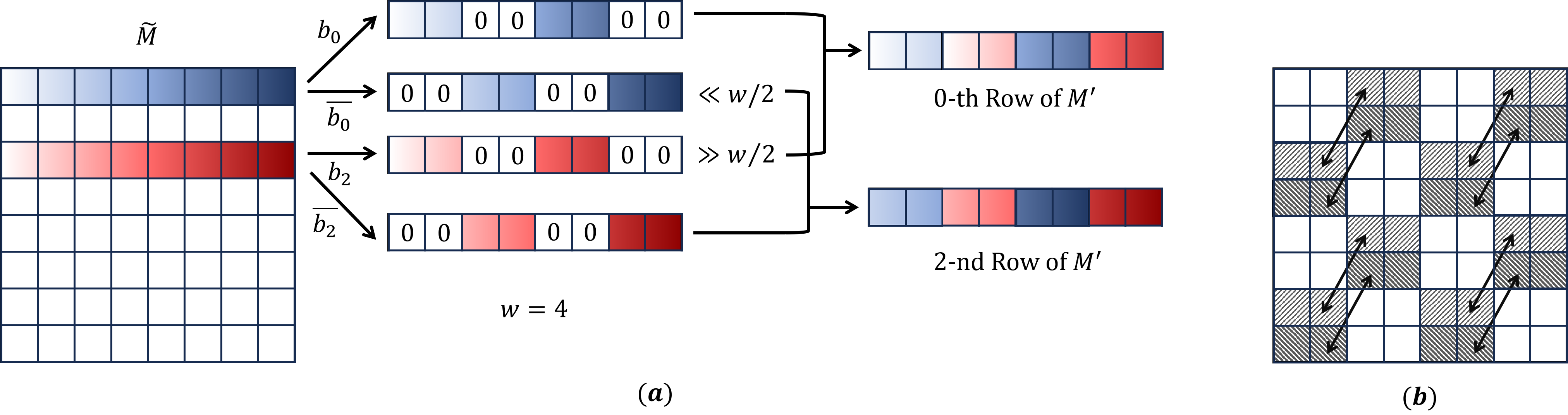
We still need show that the point-to-cell assignments can be computed efficiently.. To this end, we observe that for each point , its assignment to all nested grids can be encoded as words of length , or a bit matrix . Each row corresponds to one of the coordinates, and the most significant bit of a row indicates the assignment to cells at the highest level (i.e. cells with the largest side length) with respect to that coordinate. In other words, the most significant bits of all coordinates are packed into the first column, etc. We observe that two points and lie in the same cell of side length if and only if their matrices agree in all but the last columns. If we transpose and read the resulting matrix in the row-major order, then finding a point in the finest grid cell containing is equivalent to finding that shares the longest common prefix with . We show that this transposition can be done using simple operations on words, yielding time overall.
As an aside, we note that quadtree computation is a common task in many geometric algorithms [12]. Although an algorithm for this task was known for constant dimension [10]444Assuming that each coordinate can be represented using bits., to the best of our knowledge our algorithm is the first to achieve time for arbitrary dimension.
Step 2.
At this point we computed estimates such that . Given these estimates, importance sampling still requires sampling points. Therefore, we improve the running time by approximating (up to a constant factor) the values , as opposed to computing them exactly. This is achieved by computing random projections of the input points, which ensures that that the distance between any fixed pair of points is well-approximated with probability . We then employ these projections in a variant of the tournament algorithm of [16] which computes -approximate estimates of for sampled points in time. Since the algorithm of [16] works for the metric as opposed to the metric, we replace Gaussian random projections with Cauchy random projections, and re-analyze the algorithm.
This completes the overview of an -time algorithm for estimate the Chamfer distance up to a constant factor. To achieve a -approximation guarantee for any , we proceed as follows. First, instead of sampling points as before, we sample points . Then, we use the tournament algorithm to compute -approximations to , as before. 555Note that we could use the tournament algorithm to report -approximate answers, but then the dependence of the running time on would become quartic, as the term in the sample size would be multiplied by another term in the bound for the number of projections needed to guarantee that the tournament algorithm returns -approximate answers. Then we use a technique called rejection sampling to simulate the process of sampling points with probability proportional to . For each such point, we compute exactly in time. Finally, we use the sampled points and the exact values of in importance sampling to estimate the Chamfer distance up to a factor of .
This concludes the overview of our algorithm for the Chamfer distance under the metric. We remark that [8] also extends their result from the metric to the metric by first embedding points from to using random projections. This takes time, which exceeds the runtime of our algorithm, eliminating our improvement. However, a faster embedding method would yield an improved runtime for the Chamfer distance under the metric. We leave finding a faster embedding algorithm as an open problem.
2 Preliminaries
In this paper, we consider the regime where the approximation factor . Note that otherwise, an time bound would be close to the runtime of a naive exact computation.
In the proof of Theorem 1, we assume a Word RAM model where both the input coordinates and the memory/processor word size is bits. This model is particularly important in procedures Concatenate and Transpose, where we rely on the fact that we can shift bits and perform bit-wise AND, ADD and OR operations in constant time.
Notation.
For any integers , we use to denote the set of all integers from to . For any two real numbers such that , we use to denote the set of all reals from to . Let be the dimension of points.
For any , define for some subset of . We will omit the superscript when it is clear in the context.
3 Quadtree
In Figure 1, we show an algorithm QuadTree that outputs crude estimations of the nearest distances simulatenously for a set of points. The estimation guarantee is the same as the algorithm in [8]. While [8] achieves this using a quadtree with independent levels, which naturally introduce a runtime overhead, we show that two compressed quadtrees with dependent levels suffice. Our construction of compressed quadtrees is a generalization of [10] to high dimensions.
Input: Two size- subsets and of a metric space , such that for some bound .
Output: A set of values , such that every satisfies .
-
1.
Let . Sample two uniformly random points . For any point , define
where are the -th coordinates of , respectively.
-
2.
For each :
-
Compute and write each element of as a -bit binary string. Then can be viewed as a -by- binary matrix stored in the row-major order, whose -th entry is the -th significant bit of the -th element of . Transpose this matrix and concatenate the rows of the transpose. Denote the resulting binary string as .
-
Similarly, compute .
-
-
3.
Use as keys to sort all . Also, use as keys to sort all .
-
4.
For each :
-
Use the sort to find a that maximizes the length of the longest common prefix of and . Similarly, find a that maximizes the length of the longest common prefix of and .
-
If then output ; otherwise, output .
-
Correctness.
For any and any integer such that , let , where is the random point drawn on Line 1 in Figure 1. Observe that is related to the prefix of .
Claim 2.
Let be arbitrary. For any integer such that , if and only if and share a common prefix of length at least .
Proof.
If and share a common prefix of length at least , then in hashes and , the first bits of all coordinates are the same. and compute exactly these bits, thus . The reverse direction holds symmetrically.
Claim 2 justifies using ’s as an alternative representation of the binary string . [8] shows that has a locality-sensitive property, which will help us to bound the distance between points.
Claim 3 (Lemma A.4 of [8]).
For any fixed integer such that and any two points ,
where the probabilities are over the random choice of .
We now show that if two points have the same hash , then their distance is likely not too much greater than . A straight-forward bound follows from the diameter of the -dimensional cube.
Lemma 4.
For all , , and , the following always holds: If then .
Proof.
Observe that only if and are in the same -dimensional cube of side-length . The diameter of such a cube under the norm is . Therefore, for any and , is a necessary condition for to hold.
Moreover, using Claim 3, we can bound this ratio with respect to .
Lemma 5.
With probability at least , the following holds simultaneously for all , , and : If then .
Proof.
We show the contrapositive that with probability , implies simultaneously for all and . It suffices to argue that for any fixed pair of points and , this holds with probability at least . The lemma then follows by a union bound over pairs.
Let denote the largest integer that satisfies . Then we have
i.e., with probability at least , . Also, it is easy to see that if , then for all , , concluding the claim.
Symmetrically, if we define , the claims and lemmas above also hold for . Using these, we show that the expected outputs of the QuadTree algorithm are (crude) estimations of the nearest neighbor distances.
Theorem 6.
With probability at least , it holds for all that .
Proof.
We assume the success case of Lemma 5 for both and . Fix an arbitrary . Recall that the QuadTree algorithm finds for , which are associated with longest common prefixes of lengths , respectively. For integer , let denote the event . Observe from Claim 2 that when happens,
-
either and ,
-
or and .
Let , , and . We have
where the second inequality holds because implies that neither pair nor share a common prefix of length . Thus and by Claim 2.
Moreover, events for all form a partition of a sample space, so . Applying this and the locality sensitive properties of and , we get
Runtime analysis.
Lemma 7 (Line 2).
For any , (and ) can be computed in time.
Proof.
We assume without loss of generality that both are powers of . Computing the binary matrix representation of can be done in time since . Given this, we compute as follows.
Case 1: .
We partition the matrix into -by- square submatrices, denoted by
For each , we use a recursive subroutine to compute . See Figure 2 for a pictorial illustration of the Transpose algorithm.
Input: An -by- bit matrix where are powers of . An integer that is a power of and .
Output: An -by- matrix such that if it is partitioned into -by- square submatrices, then each submatrix is the transpose of the corresponding submatrix of at the same coordinates.
-
1.
Let
be zero-indexed and is its -th entry.
-
2.
For each integer such that :
-
(a)
Compute a -bit binary string such that for , its -th bit .
Also, compute a string .
-
(a)
-
3.
Define an -by- matrix , such that for each integer :
-
(a)
Let the -th row of be ,
where (resp. ) denote the operation of shifting a string to the right (resp. left) by bits.
-
(a)
-
4.
Output .
The correctness of the Transpose algorithm can be shown by induction on (the base- logarithm of) . When , Line 2a and 3a can be done using a constant number of operations on words. Thus we get the following runtime.
Claim 8.
Assuming the procedure runs in time.
We execute the Transpose algorithm for all , which takes . Then we can write down by concatenating rows of ’s, which takes time.
Case 2: .
We again partition the matrix into -by- square submatrices. In this case, we obtain .
Claim 9.
Given , runs in time.
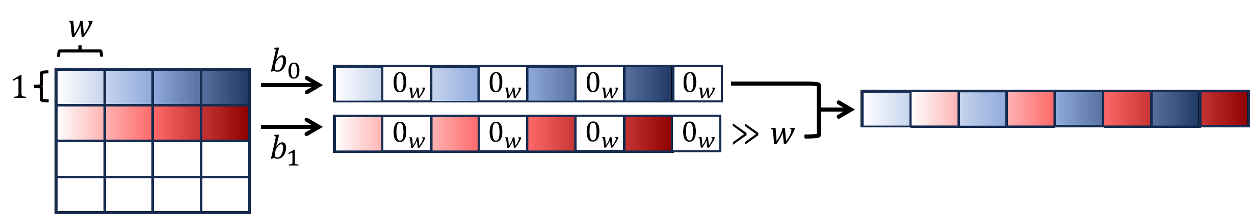
We execute and obtain . In principle, to obtain , we just concatenate rows of all . However, when , this takes longer than time. We instead use another recursive subroutine . An example of the Concatenate algorithm is given in Figure 3.
Input: An -by- bit matrix where are powers of . An integer that is a power of and .
Output: An -bit string such that if it is partitioned into -bit blocks, then the -th block (zero-indexed from left to right) are bits on the -th row of from column to .
-
1.
If then output .
-
2.
For each integer such that :
-
(a)
Partition the -th row of into -bit blocks, denoted as . Compute a -bit string , where is a -bit all-zero string.
-
(a)
-
3.
Define an -by- matrix , such that for each integer :
-
(a)
Let the -th row of be , where is the operation of shifting a string to the right by bits.
-
(a)
-
4.
Output .
The correctness of the Concatenate algorithm can again be observed by inducting on the logarithm of . Line 2a and 3a can be done using operations on words, and both lines are repeated for times in each recursive call. Therefore, the total runtime is
Theorem 10.
The QuadTree algorithm runs in time.
Proof.
Computing for all takes time. Then computing takes
time. After that, sorting -many -bit strings can be done in time using radix sort. Finally, to find with the longest common prefix for every , we go through the sorted list and link each with adjacent , which takes total time. The above time bounds also hold for ’s, resulting in time in total.
4 Tournament
In this section, we compute the -approximation of the nearest neighbor distances for logarithmically many queries. We do so using a depth- tournament. In one branch of the tournament tree, we sample a small set of input points uniformly at random. In the other branch, we partition input points into random groups, project them to a lower dimensional space, and then collect the nearest neighbor in the projected space in every group as a set . The final output of the tournament is the nearest neighbor among points in in the original space. Intuitively, if there are many (-approximate) near neighbors, then a random subset should contain one of them. And when there are few, these neighbors are likely to be assigned to different random groups, in which case the true nearest neighbor should be collected to .
Notation.
We use the same notation as in the previous section. For any finite subset , let denote the median of .
When working under the norm, we use Cauchy random variables to project points. We first recall a standard bound on the median of projections, which will be useful for our analysis. (The following lemma essentially follows from Claim 2 and Lemma 2 in [13]; we reprove it in the appendix for completeness.)
Lemma 11.
Let and . Sample random vectors . With probability at least , .
In Figure 4, we describe how to construct a data structure to find -approximate nearest neighbors. The construction borrows ideas from the second algorithm of [16], but using a tournament of depth instead of .
Input: A set of queries and a set of points , which are both subsets of a metric space .
Output: A set of values , such that every satisfies .
Building the Data Structure.
-
1.
Let .
-
2.
For each , draw , compute for all points , and store all and .
-
3.
Randomly partition into subsets , each of size .
Processing the Queries.
For each query for :
-
1.
Compute for all .
-
2.
Let be an empty set. For each :
-
Compute for every .
-
Find and add it into .
-
-
3.
Find by computing and comparing all exact distances for .
-
4.
Let be a set of samples drawn uniformly at random from . Find a point by computing and comparing all exact distances for .
-
5.
Output .
Correctness.
Fix a query . Let denote the set of all -approximate nearest neighbors to , i.e., We prove the correctness of the algorithm by casing on the size of .
Lemma 12 (Case 1).
If then with probability at least we have .
Proof.
With probability , a random sample from is in . Therefore, for containing independent samples, at least one of them is in with probability . Moreover, when this happens, it must be that . Setting gives the desired probability.
Lemma 13 (Case 2).
If then with probability at least , .
Let denote a nearest neighbor of , i.e. . To prove Lemma 13, we first make the following observation:
Lemma 14.
Let be an arbitrary subset of . The probability that there exists such that , where and , is at most .
Proof.
From we know that for any . Therefore, if then either or . Applying Lemma 11 with and and a union bound, we get that
In Line 3 of the data structure building procedure, the point is assigned to one of the subsets . If , then one can show that is likely the only -approximate nearest neighbor in . Conditioned on this, we can use Lemma 14 to show that is added into with high probability.
Lemma 15.
If , then with probability at least , is added into on Line 2 when processing the query .
Proof.
The set contains points. Since we randomly partition into , is a uniformly random subset of . When , . Conditioned on this event, we have
by Lemma 14, as long as . Therefore, with probability at least , has the smallest median of projected distance to , and thus must be added to .
Proof (of Lemma 13)..
implies that if we compute , we are guaranteed to find a nearest neighbor of , which is clearly in .
Theorem 16.
Given queries , with probability at least , the Tournament algorithm outputs -approximate nearest neighbors simulataneously for all queries.
Finally, we state the runtime guarantee as follows:
Theorem 17.
The Tournament algorithm runs in time.
Proof.
For preprocessing, the algorithm projects all points in using projections, which takes time. To process a query , we first take time to project . We then count the number of comparisons we make to find the minimums of medians, which is using a linear-time median selection algorithm [9]. Each comparison can be done in time given that and for all and are stored. Finally, we do a linear scan over and , which takes time.
We plug in and . For queries, the total runtime is .
For our purpose of estimating the Chamfer distance, we will apply the Tournament algorithm with a number of queries for and some satisfying . Under this setting, the runtime is dominated by the first additive term of Theorem 17, which is at most .
5 Rejection Sampling
Notation.
All occurrences of in this section are with respect to the set . Let be our target approximation factor. We call the distribution an -Chamfer distribution for some , if it is supported on and for every ,
We first show a general bound for estimating the Chamfer distance using samples from a Chamfer distribution. This follows from a standard analysis of importance sampling.
Lemma 18.
Let be a set of samples drawn from a -chamfer distribution . Fix . Given an arbitrarily for every that satisfies , then for any ,
where
Proof.
For the purpose of analysis, assume that we additionally have arbitrary for that also satisfies . By linearity,
We also bound the variance
where the third inequality follows from and . Finally, by Chebyshev’s Inequality, we have
In this section, we aim to construct a set of samples for some large enough , such that each is drawn from a fixed -Chamfer distribution. Once we have , we can compute a weighted sum of the nearest neighbor distances for , and invoke Lemma 18 to show that it is likely an -estimation of .
We will construct such via a two-step sampling procedure: in the first step, we sample points from using a distribution defined by the estimations from the QuadTree algorithm. In the second step, we subsample these points, using an acceptance probability defined by the estimations from the Tournament algorithm. We describe our Chamfer-Estimate algorithm in Figure 5.
Input: Two subsets of a metric space of size , a parameter , and a parameter .
Output: An estimated value .
-
1.
Execute the algorithm , and let the output be a set of values which always satisfy . Let .
-
2.
Construct a probability distribution supported on such that for every , . For , sample .
-
3.
Execute the algorithm , and let the output be a set of values which always satisfy . Let and denote (which is well-defined only if for some ).
-
4.
Define
For each , mark as accepted with probability .
If the number of accepted is less than then output Fail and exit the algorithm. Otherwise, collect the first accepted as a set .
-
5.
Compute for each . Output
The Chamfer-Estimate algorithm applies the QuadTree algorithm and the Tournament algorithm as subroutines. If they are executed successfully, their outputs should satisfy the following conditions:
Condition 19.
We say the QuadTree algorithm succeeds if for every , .
Condition 20.
We say the Tournament algorithm succeeds if for every for , .
That is, as described in the introduction, we need QuadTree to provide -approximation (to ensure that the sample size can be at most logarithmic in ), and that Tournament provide -approximation (to ensure that the final estimator using samples has variance bounded by a constant).
We state some facts about the Chamfer-Estimate algorithm, which will be useful for our analysis.
Proof.
With probability at least , by Markov’s Inequality. Upon this condition, for any ,
Proof.
Analysis of .
We now show that the set on Line 4 collects enough samples (thus the algorithm does not fail) and is equivalent to sampling from a -Chamfer distribution . We note that the algorithm, in fact, only knows a -Chamfer distribution and probabilities for , so it cannot explicitly sample from such . Nevertheless, by a standard analysis of rejection sampling, we show that “simulates” sampling from .
Proof.
We assume that Claim 21 and 22 hold. Then for any , and . Thus . The expectation is
where the second to last equality is due to the definition of . The final bound holds by Markov’s Inequality and our setting of .
Lemma 24.
Each is independently and identically distributed, and under Condition 20, for any .
Proof.
The independence and identicality follows directly from our sampling procedure. For the probability statement, we assume (without loss of generality) that during rejection sampling on Line 4, a sample is accepted and renamed as . Then for any ,
In the final equality, because we conditioned on (resp. ) on the LHS, we know that on the RHS, is well-defined and satisfy (resp. ), given Condition 20. Therefore, we have
Lemma 23 and 24 together say that can be viewed as a set of samples from a -Chamfer Distribution, thus we can invoke another importance sampling analysis. In the final step of the algorithm, we compute the exact nearest neighbor distance for all and then compute a weighted sum over them. With high probability, this gives an -estimation of .
Proof.
Theorem 26.
Chamfer-Estimate() runs in time .
Proof.
This is dominated by the runtime of QuadTree, Tournament, and the time of computing on Line 5. runs in time and Tournament runs in time. Finally, the brute-force search for for takes time.
References
- [1] Pdal: Chamfer. https://pdal.io/en/2.4.3/apps/chamfer.html, 2023. Accessed: 2023-05-12.
- [2] Pytorch3d: Loss functions. https://pytorch3d.readthedocs.io/en/latest/modules/loss.html, 2023. Accessed: 2023-05-12.
- [3] Tensorflow graphics: Chamfer distance. https://www.tensorflow.org/graphics/api_docs/python/tfg/nn/loss/chamfer_distance/evaluate, 2023. Accessed: 2023-05-12.
- [4] Arne Andersson, Torben Hagerup, Stefan Nilsson, and Rajeev Raman. Sorting in linear time? In Proceedings of the Twenty-Seventh Annual ACM Symposium on Theory of Computing, STOC ’95, pages 427–436, New York, NY, USA, 1995. Association for Computing Machinery. doi:10.1145/225058.225173.
- [5] Alexandr Andoni and Ilya Razenshteyn. Optimal data-dependent hashing for approximate near neighbors. In Proceedings of the forty-seventh annual ACM symposium on Theory of computing, pages 793–801, 2015. doi:10.1145/2746539.2746553.
- [6] Kubilay Atasu and Thomas Mittelholzer. Linear-complexity data-parallel earth mover’s distance approximations. In Kamalika Chaudhuri and Ruslan Salakhutdinov, editors, Proceedings of the 36th International Conference on Machine Learning, volume 97 of Proceedings of Machine Learning Research, pages 364–373. PMLR, 09–15 June 2019. URL: https://proceedings.mlr.press/v97/atasu19a.html.
- [7] Vassilis Athitsos and Stan Sclaroff. Estimating 3d hand pose from a cluttered image. In 2003 IEEE Computer Society Conference on Computer Vision and Pattern Recognition, 2003. Proceedings., volume 2, pages II–432. IEEE, 2003.
- [8] Ainesh Bakshi, Piotr Indyk, Rajesh Jayaram, Sandeep Silwal, and Erik Waingarten. A near-linear time algorithm for the chamfer distance, 2023. doi:10.48550/arXiv.2307.03043.
- [9] Manuel Blum, Robert W. Floyd, Vaughan Pratt, Ronald L. Rivest, and Robert E. Tarjan. Time bounds for selection. J. Comput. Syst. Sci., 7(4):448–461, August 1973. doi:10.1016/S0022-0000(73)80033-9.
- [10] Timothy M. Chan. Well-separated pair decomposition in linear time? Information Processing Letters, 107(5):138–141, 2008. doi:10.1016/j.ipl.2008.02.008.
- [11] Haoqiang Fan, Hao Su, and Leonidas J Guibas. A point set generation network for 3d object reconstruction from a single image. In Proceedings of the IEEE conference on computer vision and pattern recognition, pages 605–613, 2017.
- [12] Sariel Har-Peled. Geometric approximation algorithms. Number 173. American Mathematical Soc., 2011.
- [13] Piotr Indyk. Stable distributions, pseudorandom generators, embeddings, and data stream computation. Journal of the ACM (JACM), 53(3):307–323, 2006. doi:10.1145/1147954.1147955.
- [14] Li Jiang, Shaoshuai Shi, Xiaojuan Qi, and Jiaya Jia. Gal: Geometric adversarial loss for single-view 3d-object reconstruction. In Proceedings of the European conference on computer vision (ECCV), pages 802–816, 2018.
- [15] Omar Khattab and Matei Zaharia. Colbert: Efficient and effective passage search via contextualized late interaction over bert. In Proceedings of the 43rd International ACM SIGIR conference on research and development in Information Retrieval, pages 39–48, 2020. doi:10.1145/3397271.3401075.
- [16] Jon M. Kleinberg. Two algorithms for nearest-neighbor search in high dimensions. In Proceedings of the Twenty-Ninth Annual ACM Symposium on Theory of Computing, STOC ’97, pages 599–608, New York, NY, USA, 1997. Association for Computing Machinery. doi:10.1145/258533.258653.
- [17] Matt Kusner, Yu Sun, Nicholas Kolkin, and Kilian Weinberger. From word embeddings to document distances. In International conference on machine learning, pages 957–966. PMLR, 2015. URL: http://proceedings.mlr.press/v37/kusnerb15.html.
- [18] Erik B Sudderth, Michael I Mandel, William T Freeman, and Alan S Willsky. Visual hand tracking using nonparametric belief propagation. In 2004 Conference on Computer Vision and Pattern Recognition Workshop, pages 189–189. IEEE, 2004.
- [19] Ziyu Wan, Dongdong Chen, Yan Li, Xingguang Yan, Junge Zhang, Yizhou Yu, and Jing Liao. Transductive zero-shot learning with visual structure constraint. Advances in neural information processing systems, 32, 2019.
Appendix A Reducing the Bit Precision of Inputs
In our algorithm, we assumed that all points in input sets are integers in . Here, we show that this is without loss of generality, as long as all coordinates of the original input are -bit integers for arbitrary in a unit-cost RAM with a word length of bits.
Section of [8] gives an efficient reduction from real inputs to the case that
i.e., the input has a -bounded aspect ratio. Their reduction can be adapted to our case as follows:
Claim 27 (Lemma of [8]).
Given an such that , if there exists an algorithm that computes an -approximation to in time under the assumption that contain points from , then there exists an algorithm that computes an -approximation to for any integer-coordinate in asymptotically same time.
It remains to show how to obtain a -approximation.
Lemma 28.
There exists an -time algorithm that computes which satisfies with probability.
Proof.
Similar to (the proof of Lemma in) [8], we sample a vector , which can be discretized to -bit precision following [13]. We then compute the inner products and . The distribution of follows by the -stability property of Cauchy’s. So we have that for every and ,
with probability . Therefore, is a -approximation to . We may assume by scaling that contain -bit integers, which can be sorted in time [4]. Then to compute , we find all one-dimensional nearest neighbors by going through the sorted list and link each with adjacent , which takes time. Thus the total runtime is as claimed.
Appendix B Proof of Lemma 11
Proof.
We use the fact that for and any , . Also, for any , if a random variable then . Therefore, for any , where . The density of is , thus and
| for | ||||
Similarly, we can get . For , let be an indicator variable that equals if and equals otherwise. By Hoeffding’s bound,
which upper bounds the failure probability that the median is too small. We symmetrically bound the probability that the median is too large. Then