Identifying Approximate Minimizers Under Stochastic Uncertainity

Any solution to $\mathrm{𝖲𝖬𝖰}$ involves querying r.v.s sequentially until a $\delta$-minimum value is found. In general, the sequence of queries may depend on the realizations of previously queried r.v.s. We refer to such solutions as adaptive policies. Formally, such a solution can be described as a decision tree where each node corresponds to the next r.v. to query and the branches out of a node represent the realization of the queried r.v. Non-adaptive policies are a special class of solutions where the sequence of queries is fixed upfront: the policy then performs queries in this order until a $\delta$-minimum value is found. A central notion in stochastic optimization is the adaptivity gap [7], which is the worst-case ratio between the optimal non-adaptive value and the optimal adaptive value. All our algorithms produce non-adaptive policies and hence also bound the adaptivity gap.

Even without querying any interval, we know that the minimum value is at most $R:={\min }_{i\in N}\{r_i\}$, the minimum right-endpoint. In order to simplify notation, we incorporate this information using a dummy r.v. $X_0=[R,R]$ that is queried at the start of any policy and incurs no cost. We now formally define the condition under which a policy for $\mathrm{𝖲𝖬𝖰}$ is allowed to stop. We will refer to the partial observations at any point in a policy (i.e., values of r.v.s queried so far) as the state. Consider any state, given by a subset $S\subseteq N$ of queried r.v.s along with their observations ${\{x_i\}}_{i\in S}$. The minimum observed value is ${\min }_{i\in S}{x}_i$ and the minimum possible value among the un-queried r.v.s is ${\min }_{j\in N\setminus S}{\mathrm{\ell }}_j$. The stopping criterion is:

If this criterion is met then $\mathrm{𝖵𝖠𝖫}={\min }_{i\in S}{x}_i$ is guaranteed to satisfy $\mathrm{𝖬𝖨𝖭}\le \mathrm{𝖵𝖠𝖫}\le \mathrm{𝖬𝖨𝖭}+\delta$, where $\mathrm{𝖬𝖨𝖭}={\min }_{j\in N}{X}_j$. Also, $\arg {\min }_{i\in S}{x}_i$ is a $\delta$-minimizer. On the other hand, if this criterion is not met then there is no value $v$ that guarantees $\mathrm{𝖬𝖨𝖭}\le v\le \mathrm{𝖬𝖨𝖭}+\delta$: there is a non-zero probability that the minimum value is ${\min }_{j\in N\setminus S}{\mathrm{\ell }}_j$ or ${\min }_{i\in S}{x}_i$ (and these values are more than $\delta$ apart). So,

The stopping rule for $\mathrm{𝖲𝖬𝖰𝖨}$ is described in §2.2. An $\mathrm{𝖲𝖬𝖰𝖨}$ policy can stop either due to the $\mathrm{𝖲𝖬𝖰}$ stopping rule (above) or by inferring an un-queried interval $i^{\ast }$ as a $\delta$-minimizer.

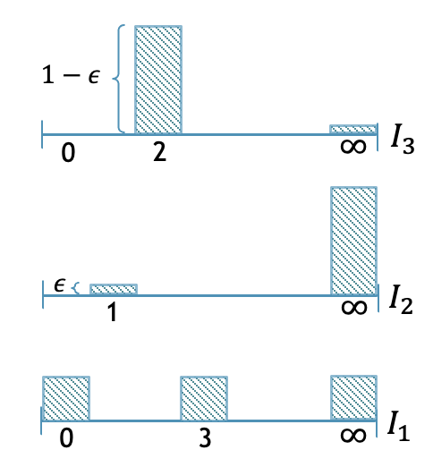
We show that the adaptivity gap for the $\mathrm{𝖲𝖬𝖰}$ problem is more than one: so adaptive policies may indeed perform better. This example also builds some intuition for the problem. Consider an instance $ℐ$ with three intervals as shown in Figure 2. In particular, $X_1\in \{0,3,\mathrm{\infty }\}$, $X_2\in \{1,\mathrm{\infty }\}$, $X_3\in \{2,\mathrm{\infty }\}$ and $\delta =1$. Let $\mathrm{Pr}(X_1=0)=\frac{1}{3},\mathrm{Pr}(X_1=3)=\frac{1}{3},\mathrm{Pr}(X_1=\mathrm{\infty })=\frac{1}{3},\mathrm{Pr}(X_2=1)=ϵ,\mathrm{Pr}(X_2=\mathrm{\infty })=1-ϵ,\mathrm{Pr}(X_3=2)=1-ϵ,\mathrm{Pr}(X_3=\mathrm{\infty })=ϵ$. An adaptive policy is shown in Figure 2, which has cost at most $1+\frac{2}{3}+\frac{ϵ}{3}=\frac{5+ϵ}{3}$. We present a case analysis in [2] and show that the best non-adaptive cost is $\min \{\frac{6-ϵ}{3},\frac{5+2ϵ}{3}\}$. Setting $ϵ=\frac{1}{3}$, we obtain an adaptivity gap of $\frac{17}{16}$. We can also modify this instance slightly to get a worse adaptivity gap of $\frac{12}{11}$.

In our analysis, we relate $\mathrm{𝖲𝖬𝖰}$ to the following simpler problem. Given $n$ r.v.s $\{X_i:i\in N\}$ with costs as before, a fixed threshold $\theta$ and budget $k$, find a policy having query-cost at most $k$ that maximizes the probability of observing a realization less than $\theta$. A useful property of this fixed threshold problem is that it has adaptivity gap one [2].

Let ${\sigma }^k$ denote the optimal policy truncated after $k$ queries: so the cost of ${\sigma }^k$ is always at most $k$. Let $L({\sigma }^k)={\min }_{i\in N\setminus {\sigma }^k}\{{\mathrm{\ell }}_i\}$ denote the smallest un-queried left-endpoint at the end of ${\sigma }^k$; this is a random value because ${\sigma }^k$ is an adaptive policy. Then,

Equality (5) is by the stopping criterion for $\mathrm{𝖲𝖬𝖰}$. The inequality in (6) uses the observation that after any $k$ queries, the smallest un-queried left-endpoint must be at most ${\mathrm{\ell }}_{k+1}$: so $L({\sigma }^k)\le {\mathrm{\ell }}_{k+1}$ always. The equality in (6) is by definition of the threshold $\theta$. Inequality (7) follows from Proposition 1.2: we view ${\sigma }^k$ is a feasible adaptive policy for the fixed-threshold problem and $T^{\ast }$ is the optimal non-adaptive policy. $◀$

Recall that each iteration $j$ of Algorithm 1 selects two intervals: $j$ in Step 3 and $b(j)$ in Step 4. Let $B=\{b(1),\mathrm{\cdots }b(2k)\}$ be the set of intervals chosen by our policy $\pi$ in Step 4 of the first $2k$ iterations. We partition $B$ into $B^{\prime }=\{b(1),\mathrm{\cdots }b(k)\}$ and $B^{\prime \prime }=\{b(k+1),\mathrm{\cdots }b(2k)\}$. Let $d^{\ast }={\text{argmin}}_{d\in T^{\ast }\setminus B}\mathrm{Pr}(X_d>{\theta }_k)={\text{argmax}}_{d\in T^{\ast }\setminus B}\mathrm{Pr}(X_d\le {\theta }_k)$.

(8) follows from the definition of $d^{\ast }$. (10) just uses that $T^{\ast }\cap B$ and $B^{\prime \prime }\setminus T^{\ast }$ are disjoint subsets of $B$. The key step above is (9), which we prove using two cases:

• $\mathrm{■}$

  Suppose that $T^{\ast }\setminus B=\mathrm{\varnothing }$. Then, using ${\theta }_k\le {\theta }_{2k}$ we obtain $\mathrm{Pr}[X_i>{\theta }_k]\ge \mathrm{Pr}[X_i>{\theta }_{2k}]$, which proves (9) for this case.

• $\mathrm{■}$

  Suppose that $T^{\ast }\setminus B\ne \mathrm{\varnothing }$. In this case, $d^{\ast }$ is well-defined. We now claim that:

  $$\text{ For each }j=k+1,\mathrm{\cdots }2k\text{, either }b(j)\in T^{\ast }\text{ or }\mathrm{Pr}[X_{b(j)}>{\theta }_{2k}]\le \mathrm{Pr}[X_{d^{\ast }}>{\theta }_k].$$

  (11)

  Indeed, consider any such $j$ and suppose that $b(j)\notin T^{\ast }$. As $d^{\ast }$ is a valid choice for $b(j)$, the greedy rule implies:

  $$\mathrm{Pr}\left[X_{d^{\ast }}>{\theta }_j\right]\ge \mathrm{Pr}\left[X_{b(j)}>{\theta }_j\right].$$

  Further, using the fact that ${\theta }_k\le {\theta }_j\le {\theta }_{2k}$, we get

  $$\mathrm{Pr}\left[X_{d^{\ast }}>{\theta }_k\right]\ge \mathrm{Pr}\left[X_{d^{\ast }}>{\theta }_j\right]\ge \mathrm{Pr}\left[X_{b(j)}>{\theta }_j\right]\ge \mathrm{Pr}\left[X_{b(j)}>{\theta }_{2k}\right],$$

  which proves (11). Let $h$ denote the number of iterations $j\in \{k+1,\mathrm{\cdots }2k\}$ where $b(j)\notin T^{\ast }$. Note that $h=|B^{\prime \prime }|-|T^{\ast }\cap B^{\prime \prime }|=k-|T^{\ast }\cap B^{\prime \prime }|\ge |T^{\ast }\setminus B|$, where we used $|T^{\ast }|=k$. Using (11), it follows that $\mathrm{Pr}[X_i>{\theta }_{2k}]\le \mathrm{Pr}[X_{d^{\ast }}>{\theta }_k]$ for all $i\in B^{\prime \prime }\setminus T^{\ast }$. Hence,

  $$\mathrm{Pr}{[X_{d^{\ast }}>{\theta }_k]}^{|T^{\ast }\setminus B|}\ge \mathrm{Pr}{[X_{d^{\ast }}>{\theta }_k]}^h\ge \prod _{i\in B^{\prime \prime }\setminus T^{\ast }}\mathrm{Pr}[X_i>{\theta }_{2k}],$$

  Combined with the fact that ${\theta }_k\le {\theta }_{2k}$ (as before), we obtain (9).

We are now ready to complete the proof. Using the $\mathrm{𝖲𝖬𝖰}$ stopping criterion and the fact that $\pi$ queries all the intervals in $B$ within $2k$ iterations,

Combined with (10),

where we use the definition $\theta ={\theta }_k$. $◀$

We note that the optimal values of $\mathrm{𝖲𝖬𝖰}$ and $\mathrm{𝖲𝖬𝖰𝖨}$ differ by at most the maximum query cost $c_{max}$. As noted above, the optimal $\mathrm{𝖲𝖬𝖰𝖨}$ value is at most that of $\mathrm{𝖲𝖬𝖰}$. On the other hand, the optimal $\mathrm{𝖲𝖬𝖰}$ value is at most the optimal $\mathrm{𝖲𝖬𝖰𝖨}$ value plus the cost to query $i^{\ast }$. In the unit-cost setting, $c_{max}=1$ and any policy has expected cost at least $1$: so the optimal values of $\mathrm{𝖲𝖬𝖰}$ and $\mathrm{𝖲𝖬𝖰𝖨}$ are within a factor two of each other. This immediately implies that Algorithm 1 is also an $8$-approximation for unit-cost $\mathrm{𝖲𝖬𝖰𝖨}$. In the rest of this subsection, we will prove a stronger result, that Algorithm 1 is a $4$-approximation for $\mathrm{𝖲𝖬𝖰𝖨}$. Apart from the improved constant factor, these ideas will also be helpful for $\mathrm{𝖲𝖬𝖰𝖨}$ with general costs. We note that under general costs, the optimal $\mathrm{𝖲𝖬𝖰}$ and $\mathrm{𝖲𝖬𝖰𝖨}$ values may differ by an arbitrarily large factor because $c_{max}$ is not a lower bound on the optimal value.

Consider any state, given by a subset $S\subseteq N$ of queried r.v.s along with their observations ${\{x_i\}}_{i\in S}$. There are two conditions under which the $\mathrm{𝖲𝖬𝖰𝖨}$ policy can stop.

• $\mathrm{■}$

  The first stopping rule is just the one for $\mathrm{𝖲𝖬𝖰}$ (1), which corresponds to the situation that interval $i^{\ast }$ is queried. We restate this rule below for easy reference:

  $$\underset{i\in S}{\min }{x}_i\le \underset{j\in N\setminus S}{\min }{\mathrm{\ell }}_j+\delta .$$

  (12)

  In this case, we return $i^{\ast }=\arg {\min }_{i\in S}{x}_i$. We refer to this as the old stopping rule.

• $\mathrm{■}$

  The second stopping rule handles the situation where an un-queried interval $i^{\ast }$ is returned. For any $i\in N$, define the “almost prefix” set . Note that either $P_i$ or $P_i\cup i$ is a prefix of $[n]$. (As before, we assume that intervals are indexed by increasing order of their left-endpoint, i.e., ${\mathrm{\ell }}_1\le {\mathrm{\ell }}_2\le \mathrm{\cdots }{\mathrm{\ell }}_n$.) The new rule is:

  $$\exists i\in N\text{ such that }{P}_i\subseteq S\text{ and }\underset{j\in P_i}{\min }{x}_j\ge r_i-\delta .$$

  (13)

  In other words, there is some interval $i$ where (1) all intervals $j\ne i$ with left-endpoint have been queried, and (2) the minimum value of these r.v.s is at least $r_i-\delta$. In this case, we return $i^{\ast }=i$ (we may not know a $\delta$-minimum value). We refer to this as the new stopping rule. See Figure 5 for an example.

Our algorithm for $\mathrm{𝖲𝖬𝖰𝖨}$ with unit costs remains the same as for $\mathrm{𝖲𝖬𝖰}$ (Algorithm 1). The only difference is in the new stopping criterion (described above). Recall that $\pi$ is the permutation used by our non-adaptive policy. When it is clear from the context, we will also use $\pi$ to denote our $\mathrm{𝖲𝖬𝖰𝖨}$ policy that performs queries in the order of $\pi$ until stopping criteria (12) or (13) applies.

We now prove this result. Let $\sigma$ denote an optimal adaptive policy for $\mathrm{𝖲𝖬𝖰𝖨}$. For any $k\ge 1$, we will show:

This would suffice to prove the $4$-approximation, exactly as in Theorem 2.2.

In order to prove (14), we fix some $k\ge 1$. As in the previous proof, let $\theta ={\theta }_k={\mathrm{\ell }}_{k+1}+\delta$ and let $T^{\ast }$ be defined as in (4). To reduce notation, define the following events.

Let $L$ denote the smallest un-queried left-endpoint at the end of iteration $2k$ in $\pi$. Note that $L$ is a deterministic value as $\pi$ is a non-adaptive policy. Moreover, $L\ge {\mathrm{\ell }}_{2k+1}$ as $\pi$ would have queried the first $2k$ r.v.s. Let $𝒢$ be the event that $X_i>L+\delta$ for all intervals $i$ queried by $\pi$ in its first $2k$ iterations. In other words, $𝒢$ is precisely the event that stopping criterion (12) does not apply at the end of iteration $2k$ in $\pi$, i.e., $𝒢=\neg {𝒜}_1$. By Lemma 2.4,

Similarly, let ${𝒢}^{\ast }$ be that event that $X_i>\theta$ for all intervals $i$ in the first $k$ queries of $\sigma$. From the proof of Lemma 2.3, we obtain ${𝒪}_1\subseteq \neg {𝒢}^{\ast }$ and

Combining the above two inequalities, we have

Let ${𝒢}_A$ be the event that $X_j>L+\delta$ for all r.v.s $j\in N$. Similarly, let ${𝒢}_A^{\ast }$ be the event that $X_j>\theta$ for all $j\in N$. Clearly,

We will now prove that

If $\sigma$ finishes due to (13) in $k$ queries then $P_{i^{\ast }}\subseteq [k+1]$: otherwise $|P_{i^{\ast }}|>k$ which contradicts with the fact that all r.v.s in $P_{i^{\ast }}$ must be queried. Let $R=\{i\in N:P_i\subseteq [k+1]\}$ be all such intervals. It now follows that the event ${𝒪}_2$ (which corresponds to policy $\sigma$) is a subset of the event

Note that $ℰ$ is independent of the policy: it only depends on the realizations of the r.v.s (and doesn’t depend on whether/not an interval has been queried).

Moreover, our policy $\pi$ queries all the r.v.s in $[2k]\supseteq [k+1]$ within $2k$ iterations. So, for all $i\in R$, the r.v.s in $P_i\subseteq [k+1]$ are queried by $\pi$ in $2k$ iterations. Hence, event ${𝒜}_2$ (which corresponds to policy $\pi$) contains event $ℰ$.

Recall that the event ${𝒢}_A$ (resp. ${𝒢}_A^{\ast }$) in policy $\pi$ (resp. $\sigma$) means that every r.v. is more than $L+\delta$ (resp. $\theta$). Also, $\theta \le L+\delta$, which means

In other words, for any $j\in N$, if $Y_j$ (resp. $Z_j$) is the r.v. $X_j$ conditioned on ${𝒢}_A$ (resp. ${𝒢}_A^{\ast }$) then $Y_j$ stochastically dominates $Z_j$.²²2We say that r.v. $Y$ stochastically dominates $Z$ if $\mathrm{Pr}[Y\ge u]\ge \mathrm{Pr}[Z\ge u]$ for all $u\in ℝ$. Note also that the r.v.s $Y_j$s (resp. $Z_j$s) are independent. Using the fact that event $ℰ$ corresponds to a monotone function, we obtain:

It suffices to prove the following.

Note that the r.v.s above only differ at position $k$. To keep notation simple, for any $j\in [n]\setminus k$ let $X_j^{\prime }=Y_j$ if and $X_j^{\prime }=Z_j$ if $j>k$. So, we need to show $\mathrm{Pr}[ℰ(X^{\prime },Y_k)]\ge \mathrm{Pr}[ℰ(X^{\prime },Z_k)]$. We condition on the realizations of the $X^{\prime }$ r.v.s. For each $j\in [n]\setminus k$ let $t_j$ denote the realization of the r.v. $X_j^{\prime }$. Having conditioned on these r.v.s, the only randomness is in $Y_k$ and $Z_k$. We will show:

Using the definition of the event $ℰ$ from (18), let $R(t)=\{i\in R:k\in P_i\text{ and }{t}_j>r_i-\delta \text{ for all }j\in P_i\setminus k\}$. In other words, $R(t)\subseteq R$ corresponds to those “clauses” in (18) that have not evaluated to true or false based on the realizations $\{X_j^{\prime }=t_j:j\in [n]\setminus k\}$. If there is some clause in (18) that already evaluates to true (based on $t$) then $ℰ$ holds regardless of $Y_k$ or $Z_k$. So, (19) holds in this case (both terms are one). Now, we assume that no clause in (18) already evaluates to true. We can write

where $f={\min }_{i\in R(t)}{r}_i-\delta$ is a deterministic value.³³3If $R(t)=\mathrm{\varnothing }$ then we set $f=\mathrm{\infty }$. Similarly, we have

Using the fact that $Y_k$ (resp. $Z_k$) is independent of $X^{\prime }$ and that $Y_k$ stochastically dominates $Z_k$,

This completes the proof of (19). De-conditioning the $X^{\prime }$ r.v.s, we obtain $\mathrm{Pr}[ℰ(X^{\prime },Y_k)]\ge \mathrm{Pr}[ℰ(X^{\prime },Z_k)]$ as desired. $◀$

Using Lemma 2.7, we obtain $\mathrm{Pr}[ℰ|{𝒢}_A]\ge \mathrm{Pr}[ℰ|{𝒢}_A^{\ast }]$, which proves (17). Combined with (16),

We have

This completes the proof of (14) and the theorem.

We handle separately the costs of intervals queried in Steps 3 and 6. The total cost incurred in Step 3 of the first $g$ iterations is $c(T_g)\le y^g$: this uses ${\cup }_{k=0}^g{T}_k=T_g$ because $T_g$ are prefixes. The total cost due to Step 6 can be bounded using a geometric series:

The inequality above is by the cost guarantee for (KP). The lemma now follows. $◀$

Recall that ${\sigma }_g$ denotes the optimal policy truncated at cost $y^g$. We let $L({\sigma }_g)={\min }_{j\in N\setminus {\sigma }_g}\{{\mathrm{\ell }}_j\}$ be the smallest un-queried left-endpoint: this is a random value as ${\sigma }_g$ is adaptive. In the algorithm, consider iteration $g$ and let $L(T_g)={\min }_{j\in N\setminus T_g}\{{\mathrm{\ell }}_j\}$; note that the threshold ${\theta }_g\ge L(T_g)+\delta$ in Step 4. Let ${\pi }^{\prime }={\pi }_{g-1}\circ T_g$ denote the list after Step 3 in iteration $g$. Note that the optimization in (KP) of iteration $g$ is over $T\subseteq N\setminus {\pi }^{\prime }$, which yields $U_g$. Also, ${\pi }_g={\pi }^{\prime }\cup U_g$.

The equality in (21) is given by the definition of $L({\sigma }_g)$ and the stopping rule. The inequality in (21) uses the fact that $L({\sigma }_g)\le L(T_g)$ always, which in turn is because ${\sigma }_g$ has cost at most $y^g$ and $T_g$ is the maximal prefix within this cost. The inequality in (22) uses ${\theta }_g\ge L(T_g)+\delta$. The inequality in (23) is by Proposition 1.2: we view ${\sigma }_g$ as a feasible adaptive policy for the fixed-threshold problem with threshold ${\theta }_g$ and budget $y^g$. The equality in (24) follows from independence of the random variables. The first equality in (25) uses the definition of $p_g^{\ast }$ from (KP) and independence. The first inequality in (26) uses the choice of $U_g$ and Theorem 3.2. The equality in (26) is by ${\pi }_g={\pi }^{\prime }\cup U_g$. To see the last inequality in (26), note that if ${\min }_{j\in {\pi }_i}\{X_j\}\le {\theta }_g$ then $\pi$ finishes by iteration $g$. $◀$

References

- [1] Marek Adamczyk, Maxim Sviridenko, and Justin Ward. Submodular stochastic probing on matroids. Math. Oper. Res., 41(3):1022–1038, 2016. doi:10.1287/MOOR.2015.0766.
- [2] Hessa Al-Thani and Viswanath Nagarajan. Identifying approximate minimizers under stochastic uncertainty, 2025. arXiv:2504.17019.
- [3] Arash Asadpour and Hamid Nazerzadeh. Maximizing stochastic monotone submodular functions. Manag. Sci., 62(8):2374–2391, 2016. doi:10.1287/MNSC.2015.2254.
- [4] Evripidis Bampis, Christoph Dürr, Thomas Erlebach, Murilo Santos de Lima, Nicole Megow, and Jens Schlöter. Orienting (hyper)graphs under explorable stochastic uncertainty. In 29th Annual European Symposium on Algorithms (ESA), volume 204 of LIPIcs, pages 10:1–10:18, 2021. doi:10.4230/LIPICS.ESA.2021.10.
- [5] N. Bansal, A. Gupta, J. Li, J. Mestre, V. Nagarajan, and A. Rudra. When LP is the cure for your matching woes: Improved bounds for stochastic matchings. Algorithmica, 63(4):733–762, 2012. doi:10.1007/S00453-011-9511-8.
- [6] Steven Chaplick, Magnús M. Halldórsson, Murilo S. de Lima, and Tigran Tonoyan. Query minimization under stochastic uncertainty. Theoretical Computer Science, 895:75–95, 2021. doi:10.1016/J.TCS.2021.09.032.
- [7] B. C. Dean, M. X. Goemans, and J. Vondrák. Approximating the stochastic knapsack problem: The benefit of adaptivity. Math. Oper. Res., 33(4):945–964, 2008. doi:10.1287/MOOR.1080.0330.
- [8] Thomas Erlebach, Michael Hoffmann, and Frank Kammer. Query-competitive algorithms for cheapest set problems under uncertainty. Theoretical Computer Science, 613:51–64, 2016. doi:10.1016/J.TCS.2015.11.025.
- [9] Thomas Erlebach, Michael Hoffmann, Danny Krizanc, Matús Mihal’Ák, and Rajeev Raman. Computing minimum spanning trees with uncertainty. In STACS, pages 277–288, 2008.
- [10] Tomás Feder, Rajeev Motwani, Rina Panigrahy, Chris Olston, and Jennifer Widom. Computing the median with uncertainty. In Proceedings of the thirty-second annual ACM symposium on Theory of computing, pages 602–607, 2000. doi:10.1145/335305.335386.
- [11] Hao Fu, Jian Li, and Pan Xu. A PTAS for a class of stochastic dynamic programs. In 45th International Colloquium on Automata, Languages, and Programming (ICALP), volume 107 of LIPIcs, pages 56:1–56:14, 2018. doi:10.4230/LIPICS.ICALP.2018.56.
- [12] Dimitrios Gkenosis, Nathaniel Grammel, Lisa Hellerstein, and Devorah Kletenik. The Stochastic Score Classification Problem. In 26th Annual European Symposium on Algorithms (ESA), pages 36:1–36:14, 2018. doi:10.4230/LIPICS.ESA.2018.36.
- [13] Ashish Goel, Sudipto Guha, and Kamesh Munagala. How to probe for an extreme value. ACM Transactions on Algorithms (TALG), 7(1):1–20, 2010. doi:10.1145/1868237.1868250.
- [14] Sudipto Guha and Kamesh Munagala. Approximation algorithms for budgeted learning problems. In 39th Annual ACM Symposium on Theory of Computing (STOC), pages 104–113. ACM, 2007. doi:10.1145/1250790.1250807.
- [15] Anupam Gupta, Ravishankar Krishnaswamy, Viswanath Nagarajan, and R. Ravi. Running errands in time: Approximation algorithms for stochastic orienteering. Math. Oper. Res., 40(1):56–79, 2015. doi:10.1287/MOOR.2014.0656.
- [16] Anupam Gupta, Viswanath Nagarajan, and Sahil Singla. Adaptivity gaps for stochastic probing: Submodular and XOS functions. In Twenty-Eighth Annual ACM-SIAM Symposium on Discrete Algorithms (SODA), pages 1688–1702. SIAM, 2017. doi:10.1137/1.9781611974782.111.
- [17] Lisa Hellerstein, Devorah Kletenik, and Srinivasan Parthasarathy. A tight bound for stochastic submodular cover. J. Artif. Intell. Res., 71:347–370, 2021. doi:10.1613/JAIR.1.12368.
- [18] Lisa Hellerstein, Naifeng Liu, and Kevin Schewior. Quickly determining who won an election. In 15th Innovations in Theoretical Computer Science Conference (ITCS), LIPIcs, pages 61:1–61:14, 2024. doi:10.4230/LIPICS.ITCS.2024.61.
- [19] Sungjin Im, Viswanath Nagarajan, and Ruben van der Zwaan. Minimum latency submodular cover. ACM Trans. Algorithms, 13(1):13:1–13:28, 2016. doi:10.1145/2987751.
- [20] Haotian Jiang, Jian Li, Daogao Liu, and Sahil Singla. Algorithms and adaptivity gaps for stochastic k-tsp. In 11th Innovations in Theoretical Computer Science Conference (ITCS), volume 151 of LIPIcs, pages 45:1–45:25, 2020. doi:10.4230/LIPICS.ITCS.2020.45.
- [21] Simon Kahan. A model for data in motion. In Proceedings of the Twenty-third Annual ACM Symposium on Theory of computing, pages 265–277, 1991.
- [22] Nicole Megow, Julie Meißner, and Martin Skutella. Randomization helps computing a minimum spanning tree under uncertainty. SIAM Journal on Computing, 46(4):1217–1240, 2017. doi:10.1137/16M1088375.
- [23] Nicole Megow and Jens Schlöter. Set selection under explorable stochastic uncertainty via covering techniques. In International Conference on Integer Programming and Combinatorial Optimization, pages 319–333. Springer, 2023. doi:10.1007/978-3-031-32726-1_23.
- [24] Danny Segev and Sahil Singla. Efficient approximation schemes for stochastic probing and prophet problems. In 22nd ACM Conference on Economics and Computation (EC), pages 793–794. ACM, 2021. doi:10.1145/3465456.3467614.
- [25] Sahil Singla. The price of information in combinatorial optimization. In Proceedings of the Twenty-Ninth Annual ACM-SIAM Symposium on Discrete Algorithms (SODA), pages 2523–2532. SIAM, 2018. doi:10.1137/1.9781611975031.161.
- [26] Weina Wang, Anupam Gupta, and Jalani K Williams. Probing to minimize. In 13th Innovations in Theoretical Computer Science Conference (ITCS 2022), volume 215, page 120, 2022.
Appendix A Multiplicative Precision
Given an instance with non-negative r.v.s and multiplicative precision , consider a new instance of with r.v.s and additive precision . Note that
An -approximately minimum value for the original instance satisfies , where . Then, satisfies , i.e., is a -minimum value for the new instance. Similarly, if is a -minimum value for the new instance then is an -approximately minimum value for the original instance.
Appendix B Bad Example for Competitive Ratio
We provide an example that rules out any reasonable competitive ratio bound for and with precision . This is in sharp contrast to the corresponding problem with exact precision () for which a constant competitive ratio is known [21]. We note that results in the online setting assume open intervals, which in our setting (with discrete r.v.s) corresponds to all left-endpoints being distinct.444Alternatively, our example can be modified into one with open intervals where the competivity ratio is still . The benchmark in the online setting is the hindsight optimum, which is the minimum number (or cost) of queries that are needed to verify a -minimum value conditioned on the realizations of the r.v.s.
Consider an instance with r.v.s with and for all . All costs are unit and the precision . We refer to the values as low values: note that any low value is a -minimum value for this instance.
We first consider the hindsight optimum. If any of the r.v.s (say ) realizes to a low value then verifying the -minimum value just requires querying , which has cost . On the other hand, the probability that none of the r.v.s realizes to a low value is : in this case the optimal verification cost is (querying all r.v.s). So the expected optimal cost is at most .
Now, consider an policy: this does not know the realizations. It is easy to see that the only way to stop querying is when some low value is observed (or all r.v.s are queried). So, the expected cost of any policy is at least . Hence the competitive ratio for is .