Bounding the WCET of a GPU Thread Block with a Multi-Phase Representation of Warps Execution
 Thomas Carle
Christine Rochange
Thomas Carle
Christine Rochange
Abstract
This paper proposes to model the Worst-Case Execution Time (WCET) of a GPU thread block as the Worst-Case Response Time (WCRT) of the warps composing the block. Inspired by the WCRT analyzes for classical CPU tasks, the response time of a warp is modeled as its execution time in isolation added to an interference term that accounts for the execution of higher priority warps. We provide an algorithm to build a representation of the execution of each warp of a thread block that distinguishes phases of execution on the functional units and phases of idleness due to operations latency. A simple formula relying on this model is then proposed to safely upper bound the WCRT of warps scheduled under greedy policies such as Greedy-Then-Oldest (GTO) or Loose Round-Robin (LRR). We experimented our approach using simulations of kernels from a GPU benchmark suite on the Accel-Sim simulator. We also evaluated the model on a GPU program that is likely to be found in safety critical systems : SGEMM (Single-precision GEneral Matrix Multiplication). This work constitutes a promising first building block of an analysis pipeline for enabling static WCET computation on GPUs.
Keywords and phrases:
GPU, WCET analysisFunding:
Louison Jeanmougin: This work was supported by a grant overseen by the French National Research Agency (ANR) as part of the CAOTIC ANR-22-CE25-0011 project.Copyright and License:
2012 ACM Subject Classification:
Computer systems organization Real-time systems ; Computer systems organization Embedded systemsSupplementary Material:
Software (ECRTS 2025 Artifact Evaluation approved artifact): https://doi.org/10.4230/DARTS.11.1.3Editors:
Renato MancusoSeries and Publisher:
1 Introduction
Machine Learning-based algorithms are progressively being introduced in real-time embedded systems to implement tasks such as planning, object detection and avoidance, trajectory computation, decision making, etc. As these algorithms generate a high computation load that can be performed in parallel to a large extent, Graphics Processing Units (GPUs) are seen as a good addition to traditional CPUs to accelerate these operations. However, for the most critical systems that undergo a stringent certification process, the adoption of GPUs incurs difficult challenges. In particular, while it is traditionally required for the certification of e.g. avionics systems, providing static timing guarantees (such as: deadlines are always met) for software executed by a GPU is currently an open problem with no general acceptable solution. In CPU-based critical systems, these guarantees are obtained through static analyzes on the software: an accurate timing model of the hardware target is used to derive an upper bound on the Worst-Case Execution Time (WCET) of the tasks composing the program. These WCET bounds are then used to perform a schedulability analysis such as a Worst-Case Response Time (WCRT) analysis to guarantee that each task always finishes before its deadline. The development of such a solution for GPU-based systems is hindered by several factors, mainly the closed nature of commercial GPU architectures combined to their inherent complexity, that slow down the development of efficient and safe models.
The major difference between the CPU and GPU execution models is that CPU code is executed by a single thread while GPU code is intended to be executed by many threads in parallel.111This might not be true for explicitly parallel CPU programs written using the pthreads library or the OpenMP API. In that case, a specific WCET analysis is required, that accounts for thread parallelism [18]. As a consequence, the WCET analysis of a GPU function (a kernel) must consider all these threads and determine when the last of them will terminate its execution.
The degree of parallelism is determined at runtime, when the kernel is launched. At that time, the number of threads that must execute the kernel is specified as a number of blocks and a number of threads per block. Each block of threads is assigned to a computing grid, called a Streaming Multiprocessor (SM). GPUs implement the Single Instruction Multiple Threads (SIMT) execution model: within a block, threads are not run one by one but instead in groups of fixed size (usually 32 threads) named warps. Within a warp, threads execute in lockstep. Whenever threads of the same warp do not follow the same execution path after a conditional branch (a situation referred to as branch divergence), both paths are executed in sequence with a hardware-controlled thread masking mechanism that ensures that each thread executes its path only.
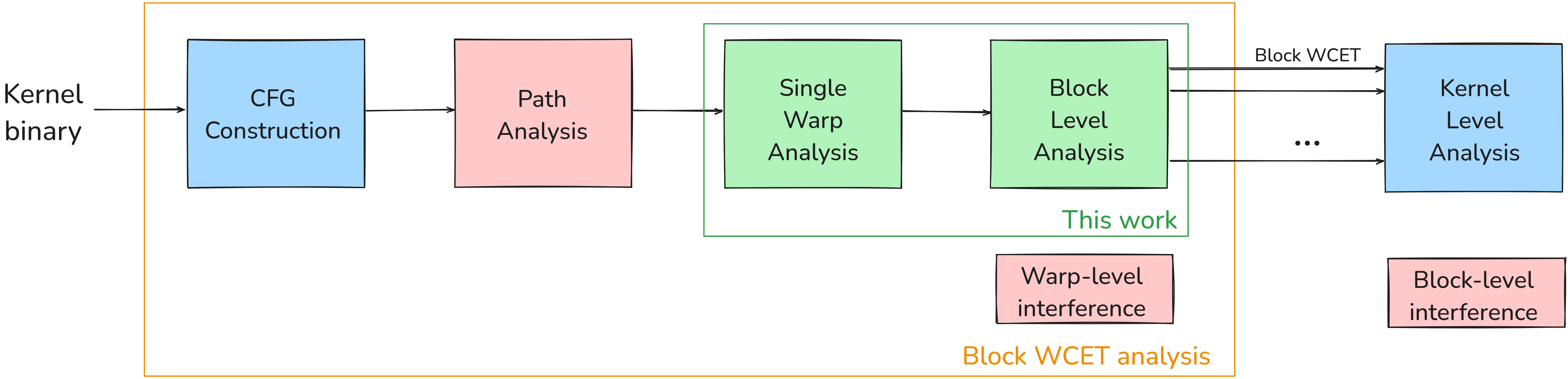
Figure 1 shows the steps required to derive the WCET of a kernel. It consists of three stages:
-
Block WCET analysis: The goal is to upper bound the WCET of a thread block executed in isolation.
-
–
CFG Construction: First of all, the Control Flow Graph (CFG) of the function must be built from the binary code. It must account for branch divergence. An approach to this step has been proposed in [13].
-
–
Path analysis: The second step uses the CFG to determine possible execution paths. The result of this step could be the set of all possible paths that should then be analyzed separately, or an abstract view of possible paths. We leave this step for future work. In this paper, we restrict ourselves to the analysis of a single path, which is derived from a simulation trace as a substitute for path analysis.
-
–
Single-Warp analysis: The WCET of a single warp running in isolation is then computed, based on a model of the GPU micro-architecture. In general, GPU vendors do not disclose details on the internals of their devices. In this paper, our GPU model is based on information collected from research papers and patents, and on a GPU simulator, Accel-Sim, that has been shown to exhibit a timing behaviour that is very close to commercial GPUs. The result of this step can be expressed as an execution profile that consists of a sequence of states for the warp. This is the first main contribution of the paper.
-
–
Warp-level memory Interference: As all the warps of a given thread block are assigned to the same SM, they may compete to access caches and shared memory, resulting in additional delays. Upper-bounding such delays is not an easy task and is left for future work. For this paper, we assume an interference-free memory system (see assumptions in Section 2).
-
–
Block-level analysis: This step aims at accounting for the interleaved execution of the warps of a thread block to derive the WCET of the whole block. This is the second main contribution of the paper.
-
–
-
Block-level memory Interference: Blocks that run on the same or on different SMs compete to access the memory system, which is likely to induce delays. As for warp-level interference, we leave the analysis of its impact for future work.
-
Kernel-level analysis: Methods to characterize the timing behaviour of a kernel (or of several kernels), including the effect of the driver and of the block schedulers, have been proposed in e.g. [9, 1, 2]. These methods assume the number of thread blocks and their WCETs are known, but do not investigate how to obtain these WCETs.
The main contribution of the paper (green boxes on the figure) is then to be seen as a building block of an approach to compute the WCET of a GPU kernel. Part of this approach is already available from the literature (blue boxes). Missing analyzes (red boxes) will be developed in future work, in some cases by expanding on already existing results e.g. scheduling rules at the block level [16, 2, 4].
The approach we propose is generic and, in time, should be applicable to any GPU, provided that sufficient information on its internals is available. Since this is currently not the case for commercial GPUs, our work uses the Accel-Sim GPU simulator [14], which is a reference for GPU simulation, as a surrogate. Although Accel-Sim does not mimic commercial GPUs with perfect cycle accuracy, its authors have shown that the simulated number of execution cycles, as well as other crucial features (e.g. number of cache misses) are strongly correlated and very close to the numbers obtained by measurements on actual commercial GPUs. We thus consider that Accel-Sim implements the constitutive elements of commercial GPUs in a representative way.
Although our proposed method does not depend on Accel-Sim, we use it here for three clearly delimited purposes:
-
It is considered as a surrogate for a commercial GPU target. We extract the timing information that we need to configure our algorithm (such as functional unit latencies) from the documentation and source code of the simulator, as we would do from the data-sheet of a commercial GPU. In time, we expect that GPU vendors that target the real-time systems market will be willing to disclose this kind of information to e.g. companies that produce WCET analyzers such as Absint.
-
It works as a substitute for the path analysis step depicted in Figure 1, that does not exist yet. It allows us to extract execution paths from a program, i.e. sequences of instructions without any timing information. These paths are used as the input of our algorithm.
-
In our evaluation, it provides the execution time at the granularity of thread blocks for standard GPU benchmarks, so that we can compare it with our WCET bounds to assess their precision.
To sum up, the paper makes the following contributions:
-
A general, multi-phase model to represent the execution of warps.
-
An algorithm to obtain the multi-phase representation of a warp execution in isolation, given a certain knowledge on the micro-architecture of the target GPU.
-
A universal formula to bound the WCET of thread blocks in isolation, that is safe for any work-conserving warp scheduling policy.
-
The evaluation of the bound using the Rodinia suite [7], and an optimized implementation of the SGEMMM algorithm.
The paper is organized as follows. Section 2 presents the fundamental assumptions that apply throughout the paper as well as the base model used to represent the execution of warps. Section 3 presents the algorithm that allows to extract the multi-phase representation of a warp in isolation, and introduces the formulas that bound the WCET of thread blocks. The evaluation of the accuracy of the bounds is provided in Section 4. Section 5 overviews related work, and Section 6 concludes the paper.
2 Assumptions and Models
As stated in the introduction, a GPU program (commonly known as a kernel ) is executed by hundreds or even thousands of threads in parallel. These threads are organized into blocks by the programmer. When a kernel is invoked by a CPU program, drivers are responsible for creating and dispatching the corresponding blocks of threads to the SMs of the GPU. Within each block, threads are grouped into sets of fixed size (which depends on the architecture of the GPU) called warps. Every cycle, one warp is selected in each SM by the warp scheduler to execute an instruction. All threads in the chosen warp run in lockstep: they all execute the same instruction at the same cycle. A consequence of this execution model is that, from a timing perspective, the behavior of the individual threads that compose a warp can be modeled by the behavior of the warp. The bounds of Section 3 capture the timing interactions between several warps that are simultaneously active on the same SM of a GPU.
The execution of a kernel by a warp amounts to the execution of a sequence of instructions . Each instruction is characterized by:
-
its opcode that determines which functional unit (FU) executes the instruction,
-
a destination register in which the instruction writes its result (if a results needs to be written),
-
zero or more source registers that hold the operands of the instruction.
In the remainder of the paper, we make the following simplifying assumptions about the basic execution mechanisms of the considered SM:
Simplifying assumption 1.
At each cycle, an SM can only issue an instruction for a single warp.
In current generations of commercial GPUs, each SM is in fact subdivided into multiple sub-cores (sometimes called SMPs). When a block is affected to a SM, each of its warps is assigned to one sub-core and does not migrate during the execution of the kernel. Our methodology can thus be extended to architectures with multiple sub-cores: first, a local WCET bound is computed for each sub-core using our method, then the effects related to components that may be shared between the sub-cores of a SM (e.g. caches, tensor units) are added to the bounds. We leave this second step as future work. For the sake of simplicity, this paper refers only to SMs, as is the case in most publications on the topic. Moreover, in current commercial GPUs, each sub-core implements a dual-issue mechanism that allows to issue up to two consecutive instructions for a warp in the current cycle, with certain restrictions. Currently we restricted our algorithm to single issue only for the sake of simplicity, but extending it should not raise any theoretical issues.
Simplifying assumption 2.
Accesses to the memory are pipelined: multiple warps of the same block can be waiting for memory requests at the same time, and these requests do not temporally interfere with each other, nor do they interfere with other functional units.
Assumption 2 is very strong and is unlikely to be verified in practice. However, we consider that the effect of memory both within a warp and across multiple warps can be modeled and conservatively bounded, with sufficient detail on the organization of the memory subsystem. Furthermore, in optimized GPU kernels, such interference effects are reduced or absorbed by relying on the shared (SRAM) memory of an SM and on asynchronous copies between shared and global memory. The design of techniques for accurately predicting the temporal behaviour of memory accesses is beyond the scope of this paper.
Simplifying assumption 3.
We do not consider a data cache in the architecture.
This assumption is equivalent to considering that all memory accesses to the global memory are cache misses. The effect of the data cache can be naturally taken into account in our model, but to our knowledge no data cache analysis exists yet for GPUs. In practice, the limitations induced by this assumption are mitigated by the fact that optimized kernels rely on the shared memory rather than on the data cache to exploit data re-use.
2.1 Warp-Level Execution Model
In order to model the properties that characterize the execution of a thread block on an SM, we propose to first model the behaviour of a single warp executing a kernel in isolation. To do so, we first enumerate a set of hardware features that are captured by our GPU execution model. These generic features either come from the literature on GPU architectures, or are directly derived from our understanding of the micro-architecture that is modelled by the Accel-Sim GPU simulator. We extracted features from the simulator as we would have done it with a real commercial GPU: we looked at the documentation and performed experiments when a clarification was needed. The main advantage of the simulator compared to a commercial GPU is the amount of documentation available, and the possibility to inspect the code of the simulator to obtain exact information about its internals. We selected the Accel-Sim simulator as a basis because its authors demonstrated a strong match between Accel-Sim and a series of modern commercial GPUs in terms of execution cycles, number of cache misses, etc. We thus believe that the hardware features that we derived from the simulator are generic features that are representative of what can be found in commercial GPUs as well, and thus constitute a generic model.
Hardware feature 1.
The considered SM is organized as a typical GPU pipeline according to the literature.
At each cycle, the frontend fetches an instruction for a given warp, and decodes an instruction that was previously fetched. The backend is responsible for selecting a warp and dispatching its next instruction to a functional unit (FU). Instructions are thus dispatched following the program order for each warp. The frontend and the backend are connected by a set of independent instruction buffers (one for each warp) that store decoded instructions.
Hardware feature 2.
Instructions of the same warp that use different FUs can be issued in consecutive cycles.
Hardware feature 3.
The FUs are partially pipelined.
When an instruction is dispatched to an FU, a certain number of cycles are spent initiating the FU for this instruction. During this time, no other instruction can be dispatched to the same FU. The rest of the execution of the instruction (the duration of which is referred to as latency) is carried out by the FU in a pipelined way: another instruction can be dispatched to the same FU in parallel. The duration of the initiation and the execution latency of an FU depend on the type of the FU, but are the same for all instructions.
In the absence of a precise documentation from COTS GPU vendors, this last feature derives from our understanding of Accel-Sim.
We also add one last simplifying assumption regarding the availability of instructions in the instruction buffers of the warps.
Simplifying assumption 4.
The instruction buffer of a warp is never empty, except when the warp has finished its execution, or after a cache miss in the instruction cache.
Assumption 4 is potentially not guaranteed in commercial GPUs. However, this property can be achieved through specific design decisions [8].
In this paper, we do not consider cache misses in the instruction cache. These could be naturally added to the proposed model if a static cache analysis were able to conservatively classify the accesses to the instruction cache. To the best of our knowledge, such an analysis does not exist yet, except for GPUs with a very particular scheduling policy [12].
Our warp-level analysis requires that the initiation and latency durations be known for each kind of operation for each type of FU: we consider that a hardware description is available that allows to map the opcodes of the instructions of to the information that characterizes the corresponding FUs:
-
an identifier of the FU,
-
the initiation duration ,
-
the latency duration .
Example 1.
Figure 2 illustrates the previous assumptions. In the top part, we consider a sequence of 5 consecutive instructions within the execution of a warp in isolation, including the instruction. Instruction is dispatched to the red FU at cycle 0. The initiation for this FU takes 2 cycles, followed by 6 cycles of latency to produce the result. At cycle 1, instruction is issued and directly dispatched to the blue FU in parallel with the initiation of instruction (Hardware feature 2), with an initiation of 3 cycles. Since instruction is also executed by the blue FU, although it is issued at cycle 2, it cannot be dispatched before the initiation of is finished (Hardware feature 3), at cycle 4. Then, its initiation starts in parallel with the latency of . Afterwards, is dependent on the destination register of , so it cannot start its initiation before produces its result at the end of cycle 8. Finally, the end of the kernel is indicated by a ret instruction, which is a special instruction not issued by the warp so it has no initiation nor latency phases. This last instruction only indicates that the kernel must finish the ongoing work before freeing the GPU resources. In that case, it translates to finishing the executions of and .
From a kernel code and a hardware description , we propose to model the execution of warps in an SM using a multi-phase model.
Definition 1.
The execution of a single warp in isolation is represented as a sequence of phases that account for the cycles during which at least an instruction is being initiated in a functional unit (execution phase) or all instructions are waiting for a result (idle phase).
Formally, each warp is represented by a sequence of phases. Each phase has the following attributes:
-
: the phase start time (cycle) relative to the block start time,
-
: the worst-case duration of the phase in cycles,
-
: the nature of the phase.
The bottom part of Figure 2 displays the multi-phase representation of the instruction sequence. The first phase accounts for the initiation of instructions , and in the 7 first cycles. Phase represents the idle cycle that results from waiting for the result produced by . Phase accounts for the initiation of and for the latencies of and .
This model exploits Hardware feature 2 at the scale of each single warp, while providing a simple and conservative abstraction of the occupancy of FUs at the scale of thread blocks. A more precise model could keep the information of which FUs are being initiated by adding FU identifiers in execution phases, in order to compute more precise block-level execution bounds. We will consider such optimizations as future work.
2.2 Block-Level Execution Model
In order to account for the effect of concurrency between warps of the same block, we add the following assumptions regarding the warp scheduling policy of the SM:
Hardware feature 4.
The scheduler is work-conserving: if at least one warp is ready to issue an instruction at a given cycle, then an instruction is issued at that cycle.
This last feature is derived from the literature on commercial GPUs e.g. [16].
Hardware feature 5.
At any given cycle, a functional unit can be performing an initiation for at most one instruction: Hardware feature 3 extends to instructions from separate warps.
Hardware feature 6.
At a given cycle, two separate FUs can be performing initiations for instructions from different warps.
Example 2.
Figure 3 illustrates the assumptions. The top part of the figure represents the actual scheduling of a block composed of two warps, each executing the same kernel as depicted in isolation in Figure 2. The execution begins with warp issuing followed by . Then at cycle 2, as is still being initiated by its FU, is issued but cannot be dispatched (which was already the case in isolation). However, the FU responsible for the execution of has finished the initiation, so it is available for a new instruction. In cycle 3, since the next instruction for depends on , it cannot be issued. As a result of this situation, the warp scheduler elects to issue and start its initiation. At cycle 4, since the initiation of for is finished, the corresponding FU is ready to initiate for . At the same time, is issued for , although it has to wait before it can be dispatched to the FU. At cycle 5, is issued for . After the initiation of for completes at the end of cycle 7, of starts its initiation on the FU. The execution of the instructions goes on until the instruction is issued by both warps and all prior instructions have completed both their initiation and latency.
When several warps coexist on the same SM, at each cycle each warp can either be issuing an instruction, initiating one or more instructions, waiting for one or more instruction results or be delayed. A delay occurs if a warp is ready to issue a new instruction to a FU, but another warp with higher priority at that moment issues an instruction, or if the warp has issued an instruction but the corresponding FU is already performing an initiation for another instruction. Our proposed multi-phase model abstracts away this complexity while providing a conservative estimation of the combined execution time of the warps composing a block. Next we describe the set of rules that define how phases from different warps of a block are combined in the multi-phase domain.
Model Rule MR 1.
At each cycle, at most one warp can be in an execution phase (Simplifying assumption 1).
Model Rule MR 2.
A warp can be in an idle phase while another warp is in an execution phase and all other warps are also in an idle phase or delayed. A warp can also be in an idle phase while all other warps are in an idle phase.
Model Rule MR 3.
A warp that begins an idle phase cannot be delayed: an idle phase starts as soon as the preceding execution phase has ended. A warp can only be delayed by execution phases of other warps.
Model Rule MR 4.
At each cycle, either one warp is in an execution phase, or all active warps (i.e. that still have phases to execute) are in an idle phase (Hardware feature 4).
These rules are compatible with the previous assumptions, but represent a conservative abstraction of how the warps actually behave. Indeed, rule MR 1 serializes the execution of phases from different warps that may correspond to actual pipelined initiations on separate FUs happening partially in parallel. However, given the complexity of the execution behaviour of the SM, we consider that this conservatism is an acceptable tradeoff to make the analysis feasible. The experiments of Section 4 show that the overall overhead induced by the method is acceptable for a wide range of benchmarks.
In the next section, we present our framework to bound the WCET of a thread block. We start by describing an algorithm that constructs the multi-phase representation of the execution of a warp in isolation. We then provide formulas to upper bound the WCET of a block and prove that the obtained bounds are effectively conservative.
3 Bounding the Block-Level WCET Using the Multi-Phase Domain
3.1 Warp-Level Timing Abstraction
| Notation | |
|---|---|
| = | kernel |
| instruction k | |
| instruction opcode | |
| destination register | |
| = | source registers |
| ret | return instruction |
| = | hardware description |
| functional unit k (identifier) | |
| initiation duration | |
| execution latency |
This section presents a procedure to build the multi-phase model for the execution of a kernel by a single warp in isolation. This procedure corresponds to the single-warp analysis box of Figure 1. The underlying algorithm is depicted by Algorithm 1. The algorithm takes as input a sequence of instructions that corresponds to the execution of , as well as a hardware description of the platform for which we construct the warp representation. The hardware description contains solely information regarding the FUs: how many FUs there are in the SM, the kind of instructions (opcodes), and for each FU, the duration of an initiation and the latency for executing an instruction. In our case, we obtained this information from the configuration file of Accel-Sim, as it determines the characteristics of our target GPU. For a commercial GPU, this information must be derived from the datasheet provided by the vendor.
As mentioned in the introduction, in the complete analysis framework, the instruction sequence representing a kernel execution is obtained from the kernel CFG. As thread divergence within warps is a crucial performance issue in GPUs, optimized kernels are often written as single path program that may include for loops with an exact static iteration bound. For such kernels, extracting the instruction sequence from the CFG is direct and does not require an additional analysis. For more complex kernels with conditional control, our algorithm can be combined with abstract interpretation to produce a multi-phase representation that encompasses the worst-case execution both in terms of execution phases and of idle phases. We leave this additional analysis for future work. In the meantime, in order to be in capacity to evaluate our algorithms and methods on generic benchmarks, we used Accel-Sim as a substitute to this path analysis step: we simulated the execution of the kernels present in our benchmark applications and extracted only the sequence of instructions executed by each of the warps, while discarding all information related to timing. Our algorithm then uses these instruction sequences in concordance with the hardware description of the target GPU to build the multi-phase representation of each warp, exactly as it would if the instruction sequences were obtained by static analysis.
The algorithm builds a sequence of alternating execution and idle phases. Each execution phase encompasses a time window in which at least one FU is performing an initiation for an instruction. Our algorithm maximizes the span of these phases: an execution phase stops only when no FU is performing an initiation, because the next instruction to be issued has pending dependencies on one or more source registers. The idle phase that follows then lasts as long as no initiation can be performed by a FU.
The algorithm uses two data structures to track the availability of the functional units () and register values () of the SM as progresses. These structures store for each FU (resp. register) the number of cycles for which it is still occupied for an initiation (resp. before its value is produced) by another instruction of . When the analysis starts, all FUs and registers are available (i.e. the number of cycles that they remain occupied is initially 0), and the first instruction to be considered is . As all FUs are available and the first instruction of does not have a source register, the first instruction belongs to the first execution phase of .
Then, for each instruction in , the algorithm checks for how long the FUs are planned to perform initiations for the previous instructions and when the source registers for the current instruction are available (Line 11). If the source registers become available before all FUs finish their ongoing initiations, the current instruction contributes to the current execution phase: it is issued in the current cycle (though it may be dispatched only later during the phase): the state of the corresponding FU and destination register are updated with the initiation and execution latencies of the instruction (Lines 23-24). Then the time advances one cycle, as the next instruction may be issued in the next cycle (Line 25). However, if the source registers are produced after all FUs finish their initiations, a time window exists when no initiation can be performed: the current execution phase stops, and an idle phase lasts until the current instruction can be dispatched to its FU. The algorithm computes the time at which the current execution finishes (when all pending initiations on all FUs are finished) (Line 12), and the start time of the next execution phase (when all the source registers for the current instruction are available). The state of the FUs is cleared, as no initiation is being performed in the idle phase. The current cycle is synchronized to the start of the new execution phase (Line 19), and the state of the registers is updated accordingly (Line 21).
When the algorithm detects the last instruction of , which is a return (ret) instruction, it closes the last execution phase and computes the duration of the last latency phase (Lines 29-35). As stated before, the ret instruction is not issued, so no initiation or latency is attached to it.
Example 3.
Let us consider again the example depicted in Figure 2. The instruction sequence of is composed of 5 instructions , with , while and have different opcodes. We consider that , and have no source registers, while . The hardware description provides the timing details e.g. with and .
The algorithm starts at time with instruction . Since has no source register and its FU is not currently occupied, it can be issued this cycle, so the algorithm skips to Line 23. The state of is updated by one initiation time: and the state of the destination register of (let us assume it is ) is updated as well: . Then time advances to 1, and the states of the FU and register are updated (latencies are decremented by one cycle). The algorithm iterates with , that is issued to with an initiation of 3 cycles, and a latency of 4 additional cycles (i.e. and ). In the meantime, time advances to 2 and the state of all currently ongoing initiations and execution latencies is decremented by one time unit (in particular, and ). In the next iteration, has no pending register dependency, so it can be issued in the current cycle. However, since its FU is the same as for , it cannot be dispatched right away. Its initiation time is thus added to the current value of the remaining initiation cycles of : and its destination register state is updated. The status of the destination register of (let us assume ) is updated: . As time advances to , the states of the FUs and registers is decremented once again. The algorithm then looks to schedule . At this point, , the latency for is equal to and the states of the FUs are: , and . Since , the algorithm stops the current execution phase. The end of phase is . At this point, the state of all FUs is set to 0. The next idle phase, starts at cycle 7 and lasts for cycle. Then, the next execution phase, starts at cycle 8. Time is increased to this cycle, and the state of the registers is decremented by 5 time units to account for this jump in time. In our example, the execution latencies of and are now consumed, meaning that their results have been written to their destination registers. However, . Since has been updated, instruction can be issued in the current cycle. As a consequence, is set to 2 and to . Then the time advances to cycle 9, so and . The next instruction is so the algorithm exits the main loop, and constructs the two last phases. The current work phase is extended to the end of the initiation of the pending instruction at cycle 10, and a last idle phase is created between cycle 10 and the moment when reaches 0 at cycle 14.
3.2 General Upper Bound for Work-Conserving Schedulers
3.2.1 Warp Scheduling Policies and their Effect on the Analysis
Determining an upper bound on the WCET of a thread block can be done in two ways: either by computing the exact schedule of the warps composing the block, or by upper-bounding the worst-case delay one warp may experience, using knowledge about the scheduling policy in a WCRT analysis fashion. Existing work report that the warp schedulers in commercial GPUs are likely to implement the Greedy-Then-Oldest (GTO) or the Loose Round Robin (LRR) scheduling policies. These two policies are not equivalent in terms of execution time performance, and it seems like none of them dominates the other. Computing the schedule at the granularity of instructions initiation and latencies amounts to simulating the execution of the kernel. However, as our objective is to derive an upper bound on the WCET of the thread block, a simulation is not enough, as the chosen input parameters for the simulation may not result in the worst situation for the execution time. On the other hand, simulating for all possible inputs is too complex to be feasible in practice. We thus propose to work at a higher abstraction level, using multi-phase representations. However, computing the schedule at this level of abstraction also suffers from two major drawbacks. First, as depicted in the bottom part of Figure 3, the initiations of the instructions of the various warps entertwine in a way that does not correspond to the phases schedule, making it problematic to relate the timing properties of the phases schedule to those of the actual instructions. Second, the durations of the execution and idle phases are only (worst-case) estimations, and as the GTO and LRR policies were not designed for predictability, they are subject to scheduling anomalies: it is possible that the schedule computed with worst-case durations is not in fact the worst-case schedule in terms of makespan. This is illustrated in Figure 4 for the LRR policy. At the top of the figure, 3 warps are scheduled with the worst-case duration assumed for each of the phases. At the bottom, the same 3 warps are scheduled with the same policy, except this time two of the phases (with stripes) spend less than their worst-case duration. At cycle 13, since only the first warp is ready, it is elected even though the round-robin order would have favored the last warp. As a result, the execution of the next phase by the last warp is postponed, which ultimately results in a lengthening of the schedule. Computing the schedule using worst-case estimations of the duration of the warps phases is thus unsafe for the GTO and LRR policies.
Another option would be to design a scheduling policy that is not subject to scheduling anomalies, in order to safely emulate a worst-case schedule and derive an upper bound on the execution time from it. The policy of [12] is an example. However, the expected gain in terms of precision of the obtained WCET for this precise example would be obtained at the cost of significant degradation of the execution time (on average 50% overhead and up to 124% overhead as reported in their experiments). Finding other policies that combine efficiency and precision is possible but outside the scope of the paper.
The only remaining option is to perform a WCRT-like analysis to bound the worst-case delay a warp may experience, by assuming only the general property of work conservation by the scheduler and abstracting away the actual policy. As we show in the remainder of the section, this is both safe and feasible using simple formulas.
3.2.2 Definition of the Bound and Proof of Correctness
We first introduce a few definitions that are then used in the proofs to correlate the actual end times of the initiation and execution of the instructions of a warp, and the bounds computed using the multi-phase representation.
Definition 2.
For any given warp that executes , any instruction , and an execution phase we denote the fact that the initiation of is abstracted in .
Definition 3.
For any given warp that executes , any instruction , and a phase we denote the fact that the end of the latency of in isolation happens in .
Definition 4.
For any given warp that executes , and a phase we denote the end of the last initiation of any instruction .
Definition 5.
For any given warp that executes , and a phase we denote the end of the latency of any instruction .
We define the phase upper-bound of a phase of warp as the sum of the durations of the phases of up to and including and of the durations of all the execution phases of all other warps in .
Definition 6.
For any warp and any phase of :
Lemma 7.
For a given warp , and any execution phase ,
Proof.
Let and such that . Then because of Hardware feature 4, can only be delayed by two causes: either its FU is already performing an initiation, or another instruction that depends on is delayed. Such an instruction is necessarily from warp . Once again because of Hardware feature 4, these delays can only be caused by the occupation of FUs by other instructions. Consequently, compared to its execution in isolation, cannot be delayed more than the number of cycles in which at least one FU is performing an initiation for an instruction of another warp. This number cannot exceed the sum of all initiation durations by all other warps, but can be less than that, since initiations on different FUs can happen in parallel. By construction, the number of cycles in which at least one FU performs an initiation for an instruction of another warp is the sum of the durations of the execution phases of the warps. By applying this reasoning to the instruction that finishes its initiation last in , we get that is less than the end of in isolation plus the sum of the execution phases of the other warps.
Lemma 8.
For a given warp , and any phase ,
Proof.
This property derives from Hardware feature 3. The feature imposes that as soon as an instruction completes its initiation on a FU, it starts executing in a fully pipelined manner: this execution does not suffer any additional delay because of other instructions. Thus, compared to the execution in isolation, the only delay the instruction can experience is the delay on the start of its initiation. The same argument we employed in the proof of Lemma 7 applies again: this delay is upper-bounded by the number of cycles in which at least one FU is performing the initiation of an instruction from another warp. Since this number is equal to the sum of the execution phases of the other warps, the lemma is proven.
Definition 9 (Warp upper bound, WUB).
For any warp in a given block :
Definition 10 (General Upper bound, GUB).
For any warp block :
Theorem 11.
For any warp block executing a kernel ,
Proof.
The proof follows from Lemma 8: for any warp , and any phase , . In particular, . In other terms, all instructions of complete their execution no later than . Since is the maximum among the for all , is greater or equal than the time at which the last instruction of any warp of completes its execution.
In the next section, we evaluate our approach, using the Accel-Sim GPU simulator. We first present the modifications that we made to the simulator in order to comply with the assumptions of the paper. Then, we evaluate the precision of the multi-phase representations produced by Algorithm 1 as well as the precision of the GUB compared to measured execution times.
4 Experiments
At this time, GPU manufacturers do not share deep and specific information about the hardware design of their accelerators. The lack of details about existing components is substantially problematic when it comes to static analysis for WCET upper-bound calculation. Formulating assumptions about the behavior of these co-processors that cannot be checked against verifiable facts might lead to wrong results if such assumptions come off as inaccurate. For these reasons, we decided to base our experiments on an open-source, configurable GPU simulator Accel-Sim [14]. The use of this simulator not only enables the access to details about the execution model of the simulated GPU, but also allows us to modify it in order to closely match our assumptions. More precisely, Hardware features 1, 2, 3, 4, 5 and 6 formalize the standard behaviour of the simulated GPU target (and are reasonable features to be encountered in commercial GPUs), while Simplifying assumptions 1, 2, 3 and 4 were enforced by modifying the configuration or source code of Accel-Sim.
4.1 Accel-Sim GPU Simulator
Accel-Sim is an open-source, configurable GPU simulator advertised to closely match the behavior of Nvidia GPUs. Formerly called GPGPU-Sim, it is able to simulate both PTX (Parallel Thread eXecution) and SASS (Streaming ASSembly) workloads. PTX is the virtual ISA (Instruction Set Architecture) for Nvidia kernels, designed for compatibility across different architectures. SASS is the machine ISA equivalent, specific to a given architecture. This simulator stands out by its adaptability, as it was developed specifically to keep up more easily with industrial advances. Indeed, Accel-Sim shows great flexibility and has many configuration options. An important feature of this simulator is that it is shipped with a set of micro-benchmarks that can be run on physical hardware in order to produce a specific configuration matching closely the hardware in question. The open source nature of this simulator coupled with its adaptability makes it a tool of choice to experiment our approach on.
Accel-Sim General Architecture
Figure 5 shows the overall architecture described in the GPGPU-Sim 4.X performance model employed in Accel-Sim. At the highest level, the GPU contains a number of SMs depending on the simulated hardware. All the SMs share an L2 cache supplied by the global memory (HBM/GDDR). Each SM contains an instruction cache shared by an arbitrary number of sub-cores. A sub-core comprises a warp scheduler, a register file and a set of functional units of different types and count. The sub-cores of an SM also share a constant cache as well as an L1 data cache and shared memory. All these elements constituting the GPU can be modified through simulator configuration or directly by tempering with the source code.
In Accel-Sim, when a GPU program is initiated by the CPU, a Thread Block Scheduler is in charge of dispatching the thread blocks to the available SMs. A thread block is dispatched to an SM if its available resources are sufficient for the execution. Limiting resources can be of different nature : amount of free shared memory, number of unoccupied registers or constant cache space. Once a block has successfully been dispatched to an SM, its warps are allocated to the SM’s sub-cores. Inside a sub-core, it is the job of the warp scheduler to select ready instructions belonging to its attributed warps from the instruction buffer. The selected instruction is then issued and dispatched to its functional unit.
Modifications
Accel-sim can be modified indirectly through a configuration file, or by directly changing the source code. For the configuration file, the starting point was a file shipped with the simulator describing the Nvidia RTX3070, which is under the Ampere architecture. The use of this specific configuration is motivated by the fact that the Jetson Orin Series were produced under the same architecture, for the embedded systems market. This file was changed so the simulated GPU contains only one SM, itself containing a single sub-core as only one thread block is considered in this paper. L1 and L2 cache were disabled since data cache analysis is out of the scope of this work. GPUs present a feature called dual-issue that allows a warp to issue two instructions at the same cycle if they are both ready and not targeted at the same functional unit. This feature was disabled to comply with Simplifying assumption 1. The instruction buffer was configured so it always holds available instructions to enforce Simplifying assumption 4. Further modifications were made to the source code of the simulator. Bank conflicts for shared memory were removed and a new functional unit was implemented to handle global memory accesses, in compliance with Simplifying assumption 2.
Analysis of a GPU Benchmark Suite
We applied our approach to the Rodinia Benchmark Suite. Rodinia is a collection of benchmarks targeted at heterogeneous calculators, comprising at least one CPU and one GPU. Therefore, it contains multiple programs executing on CPU and calling for GPU procedures to execute kernels. It is also, at the time, the most documented and maintained GPU benchmark suite. It contains a diversity of applications, making it suitable to find potential edge cases for the model. The benchmark suite was modified so that each kernel be limited to a single thread block and thus executes on a single SM. Rodinia contains 23 programs totaling 58 different kernels and 583 different calls to these kernels with varied call contexts.
Ablation Study
| Baseline vs. | Perfect I$ vs. | Dual issue vs. | Cache vs. | No cache vs. | |
|---|---|---|---|---|---|
| Perfect I$ | Single core | Single issue | No cache | Our model | |
| Mean | 111.79% | 94.01% | 99.77% | 91.90% | 234.11% |
| Std. dev. | 41.01% | 4.23% | 0.73% | 13.51% | 38.77% |
| Min | 96.94% | 27.25% | 96.65% | 34.24% | 100.25% |
| Max | 494.79% | 101.00% | 102.26% | 125.10% | 290.47% |
In order to assess the impact of our simplifying assumptions and of the corresponding modifications of the simulator on the performance of the target GPU, we conducted an ablation study, the results of which are depicted in Table 4.1. We started with the standard version of the simulator, configured to mimic a single SM from the GPU of the Jetson Orin. We call this version baseline in the ablation study. From this baseline, we incrementally remove components and features, until we obtain the configuration that complies with our simplifying assumptions and that was used for the experiments of Section 4.2. Each step of this simplification corresponds to a column in Table 4.1. In each column, two variants of the architecture are compared: for each kernel instance in the benchmark, we compute the speedup (by dividing the number of execution cycles) obtained by variant A compared to variant B, in percent, and then display the mean speedup, as well as the standard deviation and the minimum and maximum speedups across the set of benchmarks. A speedup lower than 100% means that variant B incurs a longer execution time than variant A.
The first column of Table 4.1 shows the comparison between the baseline and a variant in which accesses to the instruction cache always result in a hit. This is how we enforced Simplifying assumption 4 in our version of the simulator. As we can see, on average, this modification only incurs a speedup of 11% compared to the baseline, on the Rodinia benchmarks. In some cases, the modified version is close to 5 times faster than the baseline. Some benchmarks for which all the code holds in the instruction cache execute slightly faster in the baseline configuration, due to some timing anomalies in the memory subsystem.
In the second column, we compare a variant with four sub-cores to a variant in which only one sub-core of the SM is active (both with an instruction cache that always hits). The performance of using only one sub-core, compared to the original 4 sub-cores of the baseline, has a negligible impact on the performance (less than 6% on average). This is explained by the fact that most of the benchmarks of Rodinia are not optimized to efficiently mask the latencies induced by memory accesses in a single block. The maximum speedup of 101%, which means that the variant with one sub-core is faster than the baseline by 1%, is unexpected. After investigation, it is due to a timing anomaly related to concurrent memory accesses.
The third column compares a variant with dual instruction issue to a single issue variant (both with an instruction cache that always hits and a single sub-core). Indeed, most current commercial GPUs implement a dual-issue mechanism that allows each sub-core to issue up to two instructions per cycle, with certain restrictions. We disabled this mechanism in order to comply with Simplifying assumption 1. The ablation study shows that for the Rodinia benchmarks, the dual-issue mechanism yields a negligible impact on performance.
The fourth column compares a variant with a data cache to a variant in which the data cache has been disabled to comply with Simplifying assumption 3 (both with an instruction cache that always hits, a single sub-core and single-issue). On average, considering that there is no data cache in the architecture only slows down the execution by 9% (with a standard deviation of 13%). This is coherent with benchmarks in which either there is not much re-use of the loaded data, or the data that needs to be re-used is explicitly loaded in the shared memory. In the worst case, the performance is decreased by 65%. Some benchmarks are running faster on the cache-less variant (up to 25% faster). This happens with benchmarks in which nearly all memory accesses result in a cache miss. Indeed a cache miss takes longer than a direct access to the memory, because the cache incurs a few cycles of additional delay to determine whether the access is a hit or a miss.
Finally, the last column compares a variant with a memory coalescing mechanism with our variant, in which all memory accesses are considered coalesced and pipelined, to comply with Simplifying assumption 2 (both with an instruction cache that always hits, a single sub-core, a single-issue and no data cache). Note that our variant thus complies with all simplifying assumptions. This last variant is on average 2.3 times faster than the previous variant, with a peak at nearly 3 times faster on certain benchmarks. This is not a surprise as coalescing accesses reduces the number of memory requests and thus of cycles spent waiting for the memory to reply. Since we assume that all accesses can be coalesced, which is not true in practice, the number of transactions is significantly (and artificially) reduced, and so is the execution time.
This ablation study shows that as expected, our simplifying assumptions have an impact on the performance of the GPU. However, taken separately, three out of four of these assumptions have an average impact inferior to 12% on the execution time of the considered benchmarks. The last assumption, regarding the memory coalescence mechanism has a major impact, which tells us that relaxing this assumption should be our priority in future work.
PTX Simulation
The simulator allows the user to execute workloads either from PTX or from SASS code. As mentioned earlier, SASS is the mISA and PTX the vISA, both from Nvidia. However, SASS instructions are often poorly documented and require a huge work of reverse engineering in order to understand it properly. Moreover an Nvidia SASS program is strongly related to a particular architecture, which is not the case for PTX. For these reasons, PTX assembly is used for the simulation of kernels. The Nvidia vISA is not constrained to a particular architecture and its well documented nature allows for precise understanding of instructions behaviour and mapping to functional units.
4.2 Evaluation of the Approach
Experimental Setup
We executed GPU workloads on our modified version of Accel-sim. Execution traces of the GPU payloads are extracted from the simulations. We call kernel instance the trace resulting from a single execution of the kernel in question. This trace contains information about the order in which instructions are executed, as well as the identifier of the warp that issued them. We developed an analyzer that is able to process the trace for each warp following the procedure described in Algorithm 1. It takes as input a warp execution trace and a simulator configuration file that specifies the timing data of the FUs. From those, it produces a timed execution profile corresponding to the execution of the warp in isolation. When all the execution profiles of a thread block have been generated, the GUB can be calculated, giving an upper-bound for the WCET of the block. Some kernels contain thread synchronization barriers that temporarily pause the execution of threads until all of them have reached the barrier. From the point of view of the upper bound calculation, sections separated by thread synchronization are processed independently. Then the upper-bounds of all the sections are summed together to give the upper bound for the block. We decided to work on simulation traces to retrieve the execution path of the warps as, to the best of our knowledge, there exists no analysis that derives the worst possible path (or an abstraction of such a path) for a given GPU kernel. Yet, our approach can be used in conjunction with such an analysis when one will exist.
We start with the evaluation of the accuracy of the multi-phase models extracted using Algorithm 1. We generated a separate multi-phase model for each of the 583 kernel calls, using a configuration file from Accel-sim and the simulated traces. During the construction of the model, the procedure checks that the computed time of issue (resp. time of dispatch, time of writeback) for each instruction matches the actual issue time (resp. time of dispatch, time of writeback) in the trace. Once the multi-phase profile is created, the end time of the last phase is compared to the end time of the last instruction in the trace. Table 3 provides the results of the comparison of the end times, in the rows labeled S.w. (Single warp). For 60% of the kernel calls, the constructed profile matches every single instruction issue, dispatch, write-back and overall end times when compared to the timings from the simulator. The rest of the kernel calls make use of the instruction to generate predicates. We observed that the execution time of this instruction can vary by 1 latency cycle depending on the execution context. In order to keep our analysis conservative, the instruction is considered to always take its worst-case duration. This explains the slight overestimations (always less than 1.5%) in Table 3.
We now evaluate the accuracy of the approach as a whole, by comparing the end time obtained by computing the GUB for a given block with the end time we measure by simulating the execution of the block in Accel-sim. Multiple simulations of the Rodinia benchmark have been carried out with various global memory latencies and using both the GTO and LRR scheduling policies. A realistic value for the global memory latency would be around 200 cycles. However, considering shorter and longer latencies allows better understanding the behavior of our model. Table 3 displays the overestimation induced by the GUB compared to the actual simulation time of the blocks, for the 583 kernel calls. We display the mean of the overestimation across all kernel calls along with the associated standard deviation. We also display the maximum overestimation computed on each individual kernel call, and a weighted mean that combines the overestimations with the length of the corresponding kernels. The overestimations result from two distinct factors. First, the multi-phase model does not allow to take into account the fine-grained intertwining of initiations for instructions from separate warps. This is the abstraction cost of this model, that on the other hand simplifies the computation of the upper bound on the execution time. Second, the GUB fails to account for the masking of instruction latencies by the initiation of other phases, which is one of the principles of GPU execution. Put in terms of execution and idle phases, the inaccuracy of the GUB peaks when the combined durations of the idle phases of one warp match the combined durations of the execution phases of all the other warps in the block. Indeed, in practice the initiations corresponding to the execution phases are likely to mask the latencies corresponding to the idle phases, while the GUB sums their durations to remain conservative. Once again, this results from a trade-off between the accuracy of the method and its simplicity. The maximum overestimation (72.47%) occurs for an individual kernel scheduled with the LRR policy and with a memory latency of 25 cycles. However, the mean overestimation for the LRR scheduling policy varies between 8.21% and 26%, with a value of 12.31% when the memory latency is 200 cycles, which remains acceptable. For GTO the overestimations are slightly higher. However, since our method is agnostic about the scheduling policy, the GUB is in fact the same in both cases. The variation between LRR and GTO simply results from the fact that on average, the GTO policy yields shorter execution times on our benchmarks.
| Mem. lat. (cycles) | Policy | Mean overestim. | Max overestim. | Wgt. mean | Std. dev. |
|---|---|---|---|---|---|
| 400 | |||||
| LRR | 8.21% | 33.45% | 11.35% | 4.73% | |
| GTO | 10.68% | 34.84% | 13.87% | 3.66% | |
| S.w. | 0.03% | 0.8% | 0.07% | 0.09% | |
| 200 | |||||
| LRR | 12.31% | 40.34% | 16.83% | 6.07% | |
| GTO | 15.37% | 40.06% | 20.16% | 5.31% | |
| S.w. | 0.04% | 0.8% | 0.12% | 0.1% | |
| 100 | |||||
| LRR | 16.70% | 44.97% | 22.44% | 6.96% | |
| GTO | 19.83% | 44.37% | 26.21% | 7.89% | |
| S.w. | 0.05% | 0.8% | 0.16% | 0.12% | |
| 50 | |||||
| LRR | 19.97% | 69.83% | 26.05% | 7.88% | |
| GTO | 25.56% | 70.56% | 31.52% | 9.16% | |
| S.w. | 0.06% | 0.9% | 0.21% | 0.13% | |
| 25 | |||||
| LRR | 21.81% | 72.47% | 26.84% | 8.32% | |
| GTO | 27.88% | 60.12% | 31.83% | 8.26% | |
| S.w. | 0.07% | 1.14% | 0.24% | 0.14% | |
| 10 | |||||
| LRR | 23.46% | 49.77% | 27.86% | 8.58% | |
| GTO | 29.32% | 46.36% | 31.96% | 7.58% | |
| S.w. | 0.07% | 1.37% | 0.26% | 0.15% | |
| 5 | |||||
| LRR | 26.00% | 46.38% | 28.17% | 6.81% | |
| GTO | 27.04% | 46.67% | 30.82% | 5.91% | |
| S.w. | 0.08% | 1.47% | 0.26% | 0.15% |
S.w : Single warp
SGEMM Analysis
On top of the Rodinia benchmarks, we propose a case study on two implementations of the SGEMM (Single-precision GEneral Matrix Multiplication) algorithm. This algorithm is particularly relevant as it is likely to be used to accelerate machine learning applications such as Deep and Convolutional Neural Networks for embedded computer vision applications and autonomous driving. Basically, the objective of SGEMM is to compute the product of two input matrices.
The first implementation, labeled naive, is a direct implementation of the SGEMM algorithm, that is likely to work only on small matrices. The second implementation is an optimisation of the direct algorithm that relies on a double buffering mechanism to hide the latencies of memory copies. It is able to undertake more important workloads.
In the algorithm, the product matrix is computed using multiple thread blocks, each being is responsible for computing a tile of the product matrix. To do so, the warps composing a block need data contained in multiple tiles from both the input matrices (a row of tiles from one matrix and a column of tiles from the other). The algorithm thus works in the following fashion: a) the warps copy a tile from each of the input matrices from the (slow) global memory to a (fast) SRAM scratchpad called shared memory; b) the warps synchronize using a barrier to make sure that all the data composing the tiles is available in the shared memory; c) the warps perform the tiles multiplication and accumulate it in the result tile; d) the same sequence is performed with the two next input tiles. In the remainder of the section, we call the sequence composed of a), b) and c). Figure 6 depicts the timing of a single warp performing this algorithm. For space reasons, the global memory latency and the data processing time (the multiplication and accumulation) are reduced to 6 cycles each in the figure, which is not the case in our experiments. At cycle 0 a load from the global memory is issued and initiated, then undergoes its 6 cycles of latency. Once the load is completed at cycle 8, the data is stored into the shared memory in order to be accessible from all the warps of the block. At this point, a block level synchronization barrier prevents warps from reading segments of the shared memory before all the data has been loaded. Once all the warps have reached this barrier, they begin processing the data. Once a warp has performed its multiplications and accumulations for the current input tiles, another synchronization barrier prevents it from starting to copy data from new tiles, in case other warps are still reading data from the current tiles. This sequence then repeats until the all the input tiles attributed to the thread block have been processed. The issue with this naive implementation of the SGEMM algorithm is that for each pair of input tiles that the block processes, the duration of the copy of the data between the global and the shared memories is not hidden by computations, which degrades the overall performance of the block.
Our second SGEMM implementation, inspired by [10], uses a double buffering technique in order to mitigate the impact of global memory latency. Figure 7 gives the intuition behind this mechanism. The first part of the algorithm (up until the synchronization barrier at cycle 10) is the same as in the first version. We call this first portion of the execution in the remainder of the section. After this first synchronization, this implementation differs from the last. The algorithm still proceeds iteratively, but now, the warps start each iteration by launching an asynchronous copy of the data of the input tiles that will be processed in iteration . While the copy is ongoing, the warps execute their multiply and accumulate operations on the data that was copied in the previous iteration (for iteration 1, the data that was copied during the prologue). When their computations are over, the warps synchronize using a barrier to ensure that the asynchronous copies are completed before moving to the next iteration. To support this optimization, the data from 4 input tiles must reside in the shared memory at once (2 for the current iteration, 2 for the copies for the next iteration). The advantage of this version over the naive one is that except for the prologue, the latency of the memory copies between the global and shared memories is hidden by the latency of the multiplication operations.
These two implementation strategies show two main differences. Firstly, the for the naive version comprises two synchronization barriers while there is only one in each iteration of the double buffered version. Secondly, the double buffered version is able to hide most or all of the global memory latency, apart from the , and thus yields better GPU occupancy and execution time performance.
We implemented both versions, and simulated and analyzed them for different configurations of memory latencies and number of warps. Our implementations compute the product of a matrix of size 1024* by a matrix of size *1024, thus computing a result matrix of size 1024*1024. Table 4 provides the overestimation between the GUB and the measured execution times of the thread blocks obtained on the simulator. The GUB is consistently more accurate for the naive version than for the double buffering version. We explain this by the fact that in the naive version, the memory transfer latencies between the global and the shared memories are only very partially hidden by the execution of the instructions that perform the accesses. As discussed before one of the two sources of imprecision of our approach is that the GUB fails to account for latency hiding. When the memory latency is high, the percentage of this latency being hidden by the initiation of the copy instructions is low, which yields a high precision of the GUB. As we decrease the memory latency, the initiation of the copy instructions is able to hide a larger proportion of the copy latencies, resulting in a degradation of the precision of the GUB.
In practice, for the experiments with 32 warps, the average overestimation yielded by the GUB is around 8%, with a peak at 11.15% for the double buffering version with a memory latency of 400 cycles, which remains acceptable. The most likely case in practice corresponds to the experiment with 32 warps and a global memory latency of 200 cycles, which results in an overestimation of 8.51%. As the number of warps is decreased, the instruction execution latencies of each warp occupy a larger proportion of the execution time, relative to the overall amount of initiations. For the same reason as before, this explains why the precision of the GUB worsens as the number of warps decreases.
| Mem. lat. (cycles) | 32 warps | 16 warps | 8 warps | 4 warps | |
|---|---|---|---|---|---|
| Naive | |||||
| 400 | 5.96% | 8.67% | 11.84% | 9.36% | |
| 200 | 6.57% | 10.29% | 15.56% | 13.49% | |
| 100 | 6.93% | 11.36% | 18.47% | 17.32% | |
| 50 | 7.11% | 11.97% | 20.37% | 20.18% | |
| 25 | 7.00% | 12.31% | 21.45% | 22.00% | |
| 10 | 6.16% | 12.06% | 22.04% | 23.24% | |
| 5 | 5.87% | 11.50% | 22.03% | 23.69% | |
| Double Buffering | |||||
| 400 | 11.15% | 19.19% | 33.08% | 58.21% | |
| 200 | 8.51% | 14.12% | 23.37% | 40.40% | |
| 100 | 8.44% | 14.11% | 23.57% | 41.08% | |
| 50 | 8.39% | 14.06% | 23.65% | 41.42% | |
| 25 | 8.35% | 14.01% | 23.59% | 41.54% | |
| 10 | 8.33% | 13.98% | 23.57% | 41.59% | |
| 5 | 8.32% | 13.97% | 23.59% | 41.60% |
5 Related Work
So far, very few work has attempted to derive a safe WCET for thread blocks through static analysis. In [5], the authors propose an ILP formulation to maximize the possible makespan for warps composing a thread block, scheduled with any work-preserving warp scheduling policy, a problem very similar to the one addressed in this paper. Since they do not focus on a particular scheduling policy, their solution is not subject to scheduling anomalies. However, the resolution of their ILP does not scale, contrarily to the bounds we derive in Section 3. The authors of [12] propose to adopt the Greedy-then-strict-Round-Robin warp scheduling policy in order to improve the predictability of the blocks execution time. Their analysis also relies on an ILP formulation that is safe because the target scheduling policy is immune to scheduling anomalies. However, this policy is not work-preserving, which may result in a severe degradation of the execution time. A proof-of-concept for an ad-hoc analysis is provided in [11]. A strong assumption in this approach is that the warp schedulers implement a cycle-wise round-robin policy (each warp executes for one cycle, then yields for another warp to execute). However, the complexity of the analysis limits it to relatively short kernels, or to kernels with frequent synchronization barriers. Note that these approaches assume that blocks are running in isolation on each SM, and that warps are symmetrical.
An hybrid solution to determine the execution profile of a warp is proposed in [6]: warp execution is represented as a succession of execution and idle portions whose duration is measured by adding instrumentation points in the code and by simulating the execution on the GPGPU-sim simulator [14]. Then, the WCET of a thread block is computed as the start time of the last warp of the block added to the WCET of a single warp. This result only provides a lower bound of the block WCET, so the authors propose to add constant-time delays to account for additional interference by the other warps.
More advanced work [16, 2, 17] considers the scheduling hierarchy of GPUs at higher levels (streams and blocks), and assumes that the WCET of the blocks is known. They apply retro-engineering to commercial GPUs in order to determine or confirm their inner workings.
Finally a series of work proposes warp scheduling policies to tackle different problems. Most of these publications seek to improve the execution time of the kernel, while taking into account cache locality [19, 15, 3] or thread divergence [20]. In [21] the authors propose a new warp scheduling policy to integrate real-time tasks priorities in the warp scheduler.
6 Conclusion
We presented an approach to compute an upper bound on the worst-case execution time of thread blocks executing a GPU kernel. From a description of the inner execution timings of the GPU functional units and a sequence of instructions representing a kernel execution, we developed an analysis that extracts a multi-phase representation of the execution of the kernel. This representation is then used to derive a sound WCET bound for the execution of the kernel, using a simple analytical formula. Based on experiments using a modified version of the Accel-sim simulator on the Rodinia benchmarks and on two implementations of the SGEMM algorithm, we showed that the accuracy of the WCET bounds computed using our approach are within acceptable range of the actual measured times (on average, around 12% for a realistic memory latency configuration).
We believe that this approach represents a backbone for the static analysis of the WCET of GPU kernels, and paves the way for future improvements. As part of future work, we will define additional analyses to extend the applicability of our approach, lift the simplifying assumptions it is currently based on, and improve the overall precision of the resulting WCET bound. In particular, we will combine our main algorithm with static analyses to be able to obtain a conservative multi-phase representation of any possible execution of a kernel, thus allowing to bound the execution time of non single-path kernels without relying on execution traces. We will also work on cache analysis, memory coalescing analysis, and memory interference analysis to be able to account for those mechanisms and phenomena in our framework.
References
- [1] S. W. Ali, Z. Tong, J. Goh, and J. H. Anderson. Predictable GPU Sharing in Component-Based Real-Time Systems. In 36th Euromicro Conference on Real-Time Systems (ECRTS 2024), 2024.
- [2] Tanya Amert, Nathan Otterness, Ming Yang, James H. Anderson, and F. Donelson Smith. GPU Scheduling on the NVIDIA TX2: Hidden Details Revealed. In Real-Time Systems Symposium (RTSS), 2017.
- [3] Jayvant Anantpur and R. Govindarajan. PRO: Progress Aware GPU Warp Scheduling Algorithm. In IEEE Intl Parallel and Distributed Processing Symposium, 2015.
- [4] J Bakita and J. H. Anderson. Demystifying nvidia gpu internals to enable reliable gpu management. In 30th IEEE Real-Time and Embedded Technology and Applications Symposium, RTAS ’24, 2024.
- [5] Kostiantyn Berezovskyi, Konstantinos Bletsas, and Björn Andersson. Makespan Computation for GPU Threads Running on a Single Streaming Multiprocessor. In Euromicro Conference on Real-Time Systems (ECRTS), 2012.
- [6] Adam Betts and Alastair Donaldson. Estimating the WCET of GPU-Accelerated Applications Using Hybrid Analysis. In Euromicro Conference on Real-Time Systems (ECRTS), 2013.
- [7] Shuai Che, Michael Boyer, Jiayuan Meng, David Tarjan, Jeremy W Sheaffer, Sang-Ha Lee, and Kevin Skadron. Rodinia: A benchmark suite for heterogeneous computing. In 2009 IEEE international symposium on workload characterization (IISWC), pages 44–54. Ieee, 2009. doi:10.1109/IISWC.2009.5306797.
- [8] N. Crouzet, T. Carle, and C. Rochange. Coordinating the fetch and issue warp schedulers to increase the timing predictability of gpus. In 27th Euromicro Conference on Digital System Design, DSD 2024, Paris, France, August 28-30, 2024, pages 343–350. IEEE, 2024. doi:10.1109/DSD64264.2024.00053.
- [9] N. Feddal, G. Lipari, and H.-E. Zahaf. Towards efficient parallel GPU scheduling: Interference awareness with schedule abstraction. In Proceedings of the 32nd International Conference on Real-Time Networks and Systems, RTNS 2024, Porto, Portugal, November 6-8, 2024, 2024.
- [10] S. Gray. maxas project. https://github.com/NervanaSystems/maxas/tree/master?tab=readme-ov-file, 2023.
- [11] Vesa Hirvisalo. On Static Timing Analysis of GPU Kernels. In Workshop on Worst-Case Execution Time Analysis (WCET), 2014.
- [12] Yijie Huangfu and Wei Zhang. Static WCET Analysis of GPUs with Predictable Warp Scheduling. In International Symposium on Real-Time Distributed Computing (ISORC), 2017.
- [13] Louison Jeanmougin, Pascal Sotin, Christine Rochange, and Thomas Carle. Warp-Level CFG Construction for GPU Kernel WCET Analysis. In Workshop on Worst-Case Execution Time Analysis (WCET), 2023.
- [14] Mahmoud Khairy, Zhesheng Shen, Tor M. Aamodt, and Timothy G. Rogers. Accel-sim: An extensible simulation framework for validated gpu modeling. In 2020 ACM/IEEE 47th Annual International Symposium on Computer Architecture (ISCA), pages 473–486, 2020. doi:10.1109/ISCA45697.2020.00047.
- [15] Shin-Ying Lee, Akhil Arunkumar, and Carole-Jean Wu. CAWA: Coordinated warp scheduling and cache prioritization for critical warp acceleration of GPGPU workloads. ACM SIGARCH Computer Architecture News, 43(3S), 2015.
- [16] Ignacio Sañudo Olmedo, Nicola Capodieci, Jorge Luis Martinez, Andrea Marongiu, and Marko Bertogna. Dissecting the CUDA scheduling hierarchy: a Performance and Predictability Perspective. In IEEE Real-Time and Embedded Technology and Applications Symposium (RTAS), 2020.
- [17] Nathan Otterness and James H. Anderson. Exploring AMD GPU scheduling details by experimenting with "worst practices". Real Time Systems, 58(2), 2022. doi:10.1007/S11241-022-09381-Y.
- [18] Haluk Ozaktas, Christine Rochange, and Pascal Sainrat. Automatic WCET Analysis of Real-Time Parallel Applications. In 13th Workshop on Worst-Case Execution Time Analysis, 2013.
- [19] Timothy G. Rogers, Mike O’Connor, and Tor M. Aamodt. Cache-Conscious Wavefront Scheduling. In IEEE/ACM International Symposium on Microarchitecture, 2012.
- [20] Timothy G. Rogers, Mike O’Connor, and Tor M. Aamodt. Divergence-aware warp scheduling. In IEEE/ACM International Symposium on Microarchitecture, 2013.
- [21] Jayati Singh, Ignacio Sañudo Olmedo, Nicola Capodieci, Andrea Marongiu, and Marco Caccamo. Reconciling QoS and Concurrency in NVIDIA GPUs via Warp-level Scheduling. In Design, Automation & Test in Europe Conference (DATE), 2022.