Faster Classification of Time-Series Input Streams

Agrawal, Kunal; Baruah, Sanjoy; Guo, Zhishan; Li, Jing; Reghenzani, Federico; Yang, Kecheng; Zhao, Jinhao

doi:10.4230/LIPIcs.ECRTS.2025.13

Faster Classification of Time-Series Input Streams

Kunal Agrawal

Washington University in Saint Louis, MO, USA Sanjoy Baruah

Washington University in Saint Louis, MO, USA Zhishan Guo

North Carolina State University, Raleigh, NC, USA Jing Li

New Jersey Institute of Technology, Newark, NJ, USA Federico Reghenzani

Politecnico di Milano, Italy Kecheng Yang

Texas State University, San Marcos, TX, USA Jinhao Zhao

Washington University in Saint Louis, MO, USA

Abstract

Deep learning–based classifiers are widely used for perception in autonomous Cyber-Physical Systems (CPS’s). However, such classifiers rarely offer guarantees of perfect accuracy while being optimized for efficiency. To support safety-critical perception, ensembles of multiple different classifiers working in concert are typically used. Since CPS’s interact with the physical world continuously, it is not unreasonable to expect dependencies among successive inputs in a stream of sensor data. Prior work introduced a classification technique that leverages these inter-input dependencies to reduce the average time to successful classification using classifier ensembles. In this paper, we propose generalizations to this classification technique, both in the improved generation of classifier cascades and the modeling of temporal dependencies. We demonstrate, through theoretical analysis and numerical evaluation, that our approach achieves further reductions in average classification latency compared to the prior methods.

Keywords and phrases:

Classification, Deep Learning, Sensor data streams, IDK classifiers

Funding:

Kunal Agrawal: NSF Grant No. CCF-2106699, CCF-2107280, and PPoSS-2216971.

Sanjoy Baruah: NSF Grant No. CNS-2141256 and CPS-2229290.

Zhishan Guo: NSF Grant No. CMMI-2246672.

Jing Li: NSF Grant No. CNS-2340171, DOE ASCR Award Number DE-SC0024424.

Federico Reghenzani: NGI Enrichers Transatlantic Fellowship Programme, National Resilience and Recovery Plan (PNRR) through the National Center for HPC, Big Data and Quantum Computing.

Kecheng Yang: NSF Grant No. CNS-2104181.

Copyright and License:

© Kunal Agrawal, Sanjoy Baruah, Zhishan Guo, Jing Li, Federico Reghenzani,
Kecheng Yang, and Jinhao Zhao; licensed under Creative Commons License CC-BY 4.0

2012 ACM Subject Classification:

Computer systems organization

\rightarrow

Real-time systems

Supplementary Material:

Software: https://doi.org/10.5281/zenodo.15429421

DOI:

10.4230/LIPIcs.ECRTS.2025.13

Supplementary Material:

Software (ECRTS 2025 Artifact Evaluation approved artifact): https://doi.org/10.4230/DARTS.11.1.4

Event:

37th Euromicro Conference on Real-Time Systems (ECRTS 2025)

Editors:

Renato Mancuso

Series and Publisher:

Leibniz International Proceedings in Informatics, Schloss Dagstuhl – Leibniz-Zentrum für Informatik

1 Introduction

In order to obtain an understanding of the physical world within which they are operating, autonomous Cyber-Physical Systems (CPS’s) repeatedly sense their operating environment and attempt to classify sensed signals as representing objects from one of a pre-defined set of classes. Such classification is commonly done using classifiers that are based upon Deep Learning and related AI techniques. These classifiers need to make accurate predictions in real time, even when implemented upon edge devices with limited computational capabilities. However, most classical machine learning techniques emphasize accuracy over efficiency of implementation: classical techniques are highly accurate but can be quite time-consuming even on very simple inputs. Classifier cascades, in which very resource-efficient classifiers of limited accuracy first attempt to classify each input with more powerful (but less efficient) classifiers being used only upon inputs on which these efficient ones fail, have been proposed as a means of balancing the contrasting needs of efficiency and accuracy. Such classifier cascades may be constructed using IDK classifiers [15]. An IDK classifier is obtained from some base classifier in the following manner: if the base classifier cannot make a decision with confidence exceeding a predefined threshold, it outputs a placeholder class labeled as IDK, meaning “I Don’t Know.” Multiple IDK classifiers can be trained for a given classification problem, each offering varying execution times and likelihoods of producing a definitive class rather than IDK. Wang et al. [15] proposed organizing such collections of IDK classifiers into an IDK cascade: a linear arrangement of (some or all) the IDK classifiers that specifies the order in which they are to be called upon any input until a non-IDK classification is obtained. For applications where every input must ultimately receive a real classification, a deterministic classifier, which always produces a real class, is included as the final classifier of the IDK cascade – this deterministic classifier being unable to classify an input constitutes a system fault, potentially triggering recovery mechanisms.

Temporal dependences in input streams.

Most mobile perception pipelines require that streams of input values that are obtained by sensors each be classified. It is reasonable to hypothesize some dependence among successive inputs in such time-series readings from a single sensor source. Consider, for instance, a stream of frames recorded by a camera in an autonomous vehicle, where each designated Region of Interest (RoI) is tracked across the frames in the stream. If a specific classifier accurately identifies a RoI in one frame, it is likely to be capable of classifying the same RoI in the subsequent several frames as well, until perhaps eventually failing because the object has moved too far away and needs a more sophisticated DL model for accurate recognition. While prior work studied the problem of constructing IDK cascades [6, 5, 3], the potential inter-input dependencies were not exploited when using IDK classifier cascades, which always started by invoking the first classifier in the cascade and moving through the cascade until a non-IDK classification was returned. Agrawal et al. [2] addressed this shortcoming in the prior state of the art by conducting a methodical study of the phenomenon of temporal dependence in time-series input streams. Specifically, they (i) characterized and formally defined a particular form of dependence, which quantifies the probability that the exactly same set of classifiers in the IDK cascade return real (i.e., non-IDK) classes on consecutive inputs; (ii) proposed a schema for learning the degree of dependence that may be present in a particular input stream; and (iii) presented and evaluated algorithms that are capable of exploiting the potential presence of such dependences to speed up the average duration to successful classification.

This work.

We build upon and extend the findings of Agrawal et al. [2], a seminal work in the field of embedded edge AI that, to the best of our knowledge, was the first to explore the exploitation of temporal dependencies in time-series input streams. In this paper, we aim to further improve classification performance in such settings. Our specific contributions are as follows:

1.

We derived an improved algorithm for exploiting the form of temporal dependence. The improvement comes from the conceptual realization that simply commencing classification from a different classifier than the one at the start of the cascade is not optimal – one can achieve further reduction in average classification duration by additionally skipping classifiers within the cascade based on the classification of the previous input.
2.

For this improved algorithm to be practically useful, we needed a technical breakthrough: since skipping classifiers within the cascade is essentially equivalent to synthesizing a new cascade from the ones present in the original cascade, we needed a speedier cascade-synthesis algorithm than the previously-proposed algorithm [4] with $\Theta(n^{2})$ complexity, in order to be able to use it during online classification time for each and every continuous input. We achieved a significant improvement in efficiency by developing a linear-time $\Theta(n)$ algorithm for synthesizing cascades.
3.

Additionally, we formulated a more general notion of dependence for time-series input streams, which more accurately reflects the kinds of temporal dependence that is likely to be encountered in embedded systems. We extended our improved algorithm to effectively exploit this more general form of dependence as well. Further extending the notion of dependence to a logical endpoint, a completely general characterization of dependence via Markov Decision Processes is also discussed.
4.

We performed experimental evaluation of our improved algorithm with both the original and the more general notion of temporal dependence.

Organization.

The remainder of this manuscript is organized as follows. In Section 2, we describe the model of IDK classifiers and cascades commonly used in the embedded systems community. In Section 3, we delve into the issue of temporal dependence in sensed data: we briefly summarize the main aspects of the research that we are building on (Section 3.1), and use this to motivate our proposed modifications (Section 3.2). As stated above, we needed to make a significant improvement in runtime efficiency to a previously-proposed algorithm [4] for synthesizing cascades in order for our proposed modifications to be practically realizable – this is described in Section 4. Section 5 presents our new runtime classification algorithm, and Section 6 reports on our experimental evaluation of this new algorithm as compared to the prior state-of-the-art. In Section 7, we briefly discuss a further (and very general) extension of the model of dependence that we have considered in this paper – an area to explore in greater depth in future research. Finally, we conclude in Section 8.

2 A Real-Time Model and Practical Considerations for IDK Cascades

In this section, we briefly describe the formal model for representing IDK classifiers that was defined in Abdelzaher et al. [1], and is now commonly used in the real-time scheduling literature. We suppose that there are multiple IDK classifiers denoted $K_{1},K_{2},K_{3},\ldots,K_{n-1}$ , as well as a deterministic classifier $K_{n}$ , that have all been trained to solve the same classification problem. A probabilistic characterization of the classification capabilities of the different classifiers is provided – this may be visually represented in a Venn diagram with each region corresponding to some combination of the individual classifiers returning either a real class or IDK for an input (see Figure 1 (a) for an example with three classifiers). Each classifier $K_{i}$ is also characterized by a worst case execution time (WCET) $C_{i}$ .

Given such a collection of classifiers, an algorithm was derived [1] for constructing IDK cascades that minimize the expected duration required to achieve successful classification while optionally adhering to a specified latency constraint; this algorithm has a worst-case running time of $\mathcal{O}(4^{n})$ where $n$ denotes the number of IDK classifiers. More efficient algorithms with $\mathcal{O}(n^{2})$ worst-case running time have been obtained [4] for the special case where the IDK classifiers satisfy the containment property¹¹1Containment was called ‘full dependence’ in [4]. Agrawal et al. [2] proposed the change to ‘containment’ since ‘full dependence’ may lead to confusion with the notion of temporal dependences amongst inputs.: the set of contained classifiers can be strictly ordered from least to most powerful, such that any input successfully classified by a particular classifier in the set is also successfully classified by all more powerful classifiers (see Figure 1 (b) for a Venn diagram representation).

Figure 1: (From [2]) (a): The probability space for three IDK classifiers and one deterministic classifier. The blue, red, and brown ellipses respectively denote the regions of the probability space where the classifiers

K_{1}

,

K_{2}

, and

K_{3}

are successful (i.e., do not output IDK). The enclosing rectangle denotes the region in which the deterministic classifier is successful (i.e., all inputs). Each of the disjoint regions partitioned by the ellipses is labeled with a 3-tuple, with

K_{i}

(

\overline{K}_{i}

, respectively) denoting that the IDK classifier

K_{i}

returns a real class (resp. IDK) in this region. (b): An example Venn diagram for contained classfiers. The numbers denote the associated probabilities.

Practical Considerations for IDK Cascades.

In the broader machine learning community, IDK cascades are part of adaptive inference and dynamic neural networks that dynamically adjust effort (e.g., skip layers, select among multiple sub-models, or adapt the input resolution) based on input difficulty [11, 8, 9]. The idea of cascades is also related to anytime prediction – the computation can be truncated as soon as sufficient confidence is achieved. While IDK cascades and anytime prediction are orthogonal and incomparable to each other in terms of resource efficiency, real-time analyses for IDK cascades may be extended to anytime prediction. For instance, early-exit networks can be considered as an internal realization of the contained IDK cascade, where a single deep network is augmented with multiple intermediate classifiers (exits) so that inference can “exit” early if an earlier layer’s prediction is confident [12, 10]. Here, the cost of skipping intermediate classifiers needs a modified analysis. Techniques on model compression, such as model quantization, pruning, and knowledge distillation, can also be combined with cascades. For example, more aggressively quantized models can serve as faster yet less accurate classifiers in the contained IDK cascade. These techniques all aim to balance accuracy and efficiency, a trade-off at the heart of the IDK cascade design philosophy. Recent work [14] has demonstrated the effectiveness of IDK cascades in various domains, including autonomous systems, real-time surveillance, and industrial automation, further supporting the relevance and practicality of IDK cascades.

From an implementation perspective, IDK cascades can be executed such that the follow-up model in the cascade is pre-loaded onto the computing devices (e.g., GPU) during the running of the current model to reduce runtime overhead. Depending on the available computation capacity of the application domain (e.g., real-time monitoring using IoT micro-controllers, object classification on autonomous vehicles, traffic control or smart manufacturing on the edge, city-wide surveillance system on the cloud), the number of models in such cascades can range from a dozen to several hundred.

In many application domains, like perception for autonomous driving, models are frequently pre-trained on the same or highly similar datasets. In such settings, larger and deeper models tend to consistently outperform smaller ones across most input types, giving rise to contained IDK cascades, where every input classified by a simpler model is also correctly classified by all more complex models in the cascade. Similarly, techniques like model compression and anytime prediction also naturally result in contained classifiers. Even in cases where this containment property is not strictly satisfied, the discrepancy is often minor, making it practical to approximate real-world cascades as contained with negligible loss in performance.

3 Temporal Dependences in Time-Series Input Streams

As stated in Section 2, earlier cascade-synthesis algorithms [1, 4] have been shown to be optimal for minimizing expected duration to successful classification. These optimality results, however, only hold under the assumption that there is no dependence between different inputs that are to be classified: each input is assumed to have been drawn independently from the underlying probability distribution. Focusing on the case of contained classifiers, Agrawal et al. [2] sought to exploit the possibility that some dependence between successive inputs is likely to be present. They formalized a quantitative metric of dependence in time-series input streams (Definition 1 below) in order to further reduce the average classification time.

Let $\vec{x}\stackrel{{\scriptstyle\mbox{def}}}{{=}}\langle x_{1},x_{2},x_{3}\ldots\rangle$ denote a stream of inputs to be classified (i.e., the inputs $x_{1},x_{2},x_{3},\ldots$ must each be classified, one at a time in increasing order of the subscript) by a particular IDK cascade $\mathcal{K}$ . Two inputs in $\vec{x}$ are defined to be equivalent inputs if and only if exactly the same set of classifiers in $\mathcal{K}$ would return real (i.e., non-IDK) classes upon both inputs. The defined dependence parameter $\lambda$ of input stream $\vec{x}$ with respect to $\mathcal{K}$ is a quantitative metric of the likelihood that successive inputs are equivalent inputs.

Definition 1 (dependence parameter $\lambda$ ).

Time-series input stream $\vec{x}\stackrel{{\scriptstyle\mbox{def}}}{{=}}\langle x_{1},x_{2},x_{3}\ldots\rangle$ that is to be classified by cascade $\mathcal{K}$ has dependence parameter $\lambda$ , $0\leq\lambda\leq 1$ , if and only if for each $t>1$ the input $x_{t}$ is

$\blacksquare$

with probability $\lambda$ , equivalent to the input $x_{t-1}$ ; and
$\blacksquare$

with probability $\left(1-\lambda\right)$ , drawn at random from the underlying probability distribution.

Thus, a small value of $\lambda$ indicates little dependence between successive inputs (streams where each input is independently drawn from the underlying distribution have $\lambda=0$ ) and larger $\lambda$ denotes greater dependence (when $\lambda=1$ all the inputs are equivalent inputs – they are successfully classified by exactly the same set of classifiers in the cascade $\mathcal{K}$ ).

Note that since temporal dependence is primarily a property of an input stream, having a single dependence ( $\lambda$ ) parameter to model its impact upon all the classifiers in the cascade is an oversimplification. Greater modeling accuracy (and a consequent additional reduction in classification duration) can be achieved by having one parameter to model the effect of the stream’s temporal dependence on each classifier. In Section 5.1, we proposed this more general model and adapted our algorithm to be compatible with this generalized model.

Some Notations.

In the remainder of this paper, we will often let $\mathcal{K}\stackrel{{\scriptstyle\mbox{def}}}{{=}}\left\langle K_{1},K_{2},% \ldots,K_{N}\right\rangle$ denote the static cascade – the optimal contained IDK cascade in the absence of dependencies between successive inputs, where the classifiers are listed in the order they are to be called, with $K_{N}$ denoting the deterministic classifier.²²2Note the change in notation from Section 2 – there the subscripts were just for distinguishing amongst $n$ different classifiers, whereas the subscript now denotes the position of the classifier in the optimal cascade (which comprises $N$ classifiers). Such an optimal IDK cascade can be constructed from all available classifiers using algorithms provided by Baruah et al. [4]. We let $C_{i}$ denote $K_{i}$ ’s WCET, and $P_{i}$ the probability that $K_{i}$ returns a true class (rather than IDK) upon a randomly-drawn input. (Note that $P_{N}=1$ , and that $C_{i-1}<C_{i}$ and $P_{i-1}<P_{i}$ for each $i,1<i\leq N$ , in any optimal cascade.) An example cascade for the case $N=4$ (i.e., constituting three IDK classifiers and one deterministic classifier) is depicted in Figure 2 – this optimal cascade was synthesized from the collection of contained classifiers depicted in Figure 1 (b) – as can be seen, all four classifiers appear in this optimal cascade.

$K_{i}$	$K_{1}$	$K_{2}$	$K_{3}$	$K_{4}$
$C_{i}$	$1$	$11$	$100$	$200$
$P_{i}$	$0.1$	$0.2$	$0.9$	$1.0$

Figure 2: An example cascade

\mathcal{K}=\left\langle K_{1},K_{2},K_{3},K_{4}\right\rangle

of contained classifiers.

K_{4}

is the deterministic classifier.

C_{i}

denotes the WCET of

K_{i}

, and

P_{i}

the probability that

K_{i}

will return a real (i.e., non-IDK) classification on an input drawn at random from the underlying probability distribution.

Suppose that during the classification of a particular input stream $\vec{x}$ that has dependence parameter $\lambda$ , the classifier $K_{b}$ is the first classifier in the cascade $\mathcal{K}$ to successfully classify the input $x_{t-1}$ (in Section 3.1, we will refer to $K_{b}$ as the boundary classifier for $x_{t-1}$ ). By definition of the dependence parameter (Definition 1), there is a probability $\lambda$ that $K_{b}$ will also be the first classifier to successfully classify $x_{t}$ due to dependence, and a probability $(1-\lambda)$ that $x_{t}$ will be drawn independently from the underlying probability distribution. The probability $\widehat{P_{i}}$ that each $K_{i}$ will successfully classify $x_{t}$ , is therefore as follows:

\widehat{P}_{i}=\left\{\begin{array}[]{l l}(1-\lambda)P_{i},&i<b\\ \lambda+(1-\lambda)P_{i},&i\geq b\end{array}\right.

(1)

Problem Considered.

We assume that a stream of inputs arrives (e.g., from a sensor) at the cascade with successive inputs arriving exactly $T$ time units apart. Each input must be classified before the next input arrives: i.e., there is a hard deadline of time-duration $T$ for successful classification. The performance objective is to reduce the average duration to successful classification over all the inputs in the input stream, subject to the hard deadline being met for each and every input. Once the classification is obtained for an input, the identified class is immediately reported; the lapsed duration between the input’s arrival instant and this classification instant constitutes the response time for this input. After the classification is completed, the remainder of the time-interval may be used by the runtime algorithm for performing additional “exploratory” computations that are aimed at reducing the average duration for classification of future inputs.

3.1 The Current State-of-the-art Classification Algorithm [2]

Agrawal et al. [2] present an algorithm for using the static cascade assuming the value of $\lambda$ is known³³3They describe [2] how the value of $\lambda$ can be learned via runtime observations by a direct and straightforward application of the standard learning technique of Maximum Likelihood Estimation (MLE) [13].. During an initialization phase prior to processing the input stream $\vec{x}$ , this algorithm (i) computes a “skip factor” which is a positive integer $k$ , $0\leq k\leq N$ , as a function of the value of the dependence parameter $\lambda$ characterizing $\vec{x}$ ; and (ii) designates the classifier $K_{1}$ as the boundary classifier for the classification of a hypothetical input $x_{0}$ . After this initialization phase, the algorithm proceeds to process each input in $\vec{x}$ in order, where classification is followed by an exploration step:

1.

classification. Let $b$ denote the index of the boundary classifier $K_{b}$ for $x_{t-1}$ (i.e., the earliest classifier is that can successfully classified $x_{t-1}$ ). The attempt to classify $x_{t}$ begins at the classifier $K_{\max(1,b-k)}$ , and proceeds down the cascade until a successful classification is obtained.
2.

exploration. Immediately when a successful classification for $x_{t}$ is obtained, it is reported. The reminder of the interval prior to the arrival of the next input is used to execute additional classifiers in order to determine the boundary classifier for $x_{t}$ , unless the boundary is already identified during classification.

The rationale for the design of this algorithm is motivated by considering the boundary cases: when $\lambda=0$ (no dependence) and $\lambda=1$ (full dependence).

$\blacksquare$

If $\lambda=0$ , then each input is independent and hence one should attempt to classify the input $x_{t}$ starting at classifier $K_{1}$ , working one’s way down the cascade until a successful (i.e., non-IDK) classification is obtained. By the optimality of the static cascade in the absence of input dependencies, doing so minimizes the expected classification duration.
$\blacksquare$

If $\lambda=1$ , then there is no point in attempting to classify $x_{t}$ with classifiers before $K_{b}$ – they’re all guaranteed to fail since $x_{t}$ and $x_{t-1}$ are equivalent inputs and thus successfully classified by exactly the same classifiers. Instead, using $K_{b}$ to classify $x_{t}$ is optimal.

Thus, for the two extreme values of the dependence parameter, $\lambda=0$ and $\lambda=1$ , the optimal strategy is to either start at the beginning of the cascade (when $\lambda=0$ ), or at the boundary classifier itself (when $\lambda=1$ ), respectively. For values of $\lambda$ that lie between these two extremes (i.e., $0<\lambda<1$ ), they adopt the reasonable strategy of interpolating between these optimal decisions for the two extremes and skipping backwards a constant number of classifiers $k$ (the skip factor) from the boundary classifier, where the value of $k$ depends upon the value of $\lambda$ : the smaller the value of $\lambda$ , the larger the value of $k$ .

For stream-classification algorithms based on the skip factor approach (i.e., using cascades that start processing each input a skip factor prior to the boundary classifier for the previous input), their algorithm [2] for computing the skip factor as a function of $\lambda$ is optimal: for a given value of $\lambda$ , this algorithm computes the skip factor that will result in minimum average classification time for a time series input stream with dependence parameter $\lambda$ .

3.2 Can the Skip Factor Approach be Improved?

In effect, the skip factor approach truncates the cascade for the purposes of classifying $x_{t}$ , by snipping off a segment at the front of the cascade. While the skip factor can be optimally computed, it behooves us to wonder whether one can do even better than the skip factor approach; the following example suggests the answer is ‘yes.’

Example 2.

Consider an input stream $\vec{x}$ that is to be classified by the example cascade of Figure 2, with a dependence parameter $\lambda=0.75$ . Let us suppose that the boundary classifier for the input $x_{t-1}$ is $K_{3}$ . The updated probabilities of successful classification of $x_{t}$ by the different classifiers, computed according to Equation 1, are

	$\displaystyle\widehat{P_{1}}=$	$\displaystyle(1-\lambda)\times P_{1}=0.25\times 0.1=\bm{0.025}$
	$\displaystyle\widehat{P_{2}}=$	$\displaystyle(1-\lambda)\times P_{2}=0.25\times 0.2=\bm{0.050}$
	$\displaystyle\widehat{P_{3}}=$	$\displaystyle\lambda+(1-\lambda)P_{3}=0.75+0.25\times 0.9=\bm{0.975}$
	$\displaystyle\widehat{P_{4}}=$	$\displaystyle\lambda+(1-\lambda)P_{4}=0.75+0.25\times 1.0=\bm{1}$

As the skip factor is bounded by the length of the cascade $N=4$ , i.e., $k\in\{0,1,2,3,4\}$ , let us consider every possibility.

1.

For $k\in\{2,3,4\}$ , $\max(1,3-k)=1$ . Hence the skip factor algorithm would attempt to classify $x_{t}$ starting at classifier $K_{1}$ , and the expected duration to successful classification is

$\displaystyle C_{1}+(1-\widehat{P_{1}})\times C_{2}+(1-\widehat{P_{2}})\times C% _{3}+(1-\widehat{P_{3}})\times C_{4}$

$\displaystyle=$ $\displaystyle 1+0.975\times 11+0.95\times 100+0.025\times 200=\bm{111.725}$
2.

For $k=1$ , we have $\max(1,3-1)=2$ . Hence the skip factor algorithm would attempt to classify $x_{t}$ starting at classifier $K_{2}$ and the expected duration to successful classification is

$\displaystyle C_{2}+(1-\widehat{P_{2}})\times C_{3}+(1-\widehat{P_{3}})\times C% _{4}$

$\displaystyle=$ $\displaystyle 11+0.95\times 100+0.025\times 200=\bm{111.0}$
3.

For $k=0$ , $\max(1,3-0)=3$ . Hence the skip factor algorithm would attempt to classify $x_{t}$ starting at classifier $K_{3}$ itself and the expected duration to successful classification is

$\displaystyle C_{3}+(1-\widehat{P_{3}})\times C_{4}=100+0.025\times 200=\bm{10% 5.0}$

If, however, as an alternative to the skip-factor approach, we were to instead attempt to classify $x_{t}$ using the classifiers in the order $K_{1}$ followed by $K_{3}$ and finally $K_{4}$ (i.e., we used the cascade $\left\langle K_{1},K_{3},K_{4}\right\rangle$ ), the expected duration to successful classification is

\displaystyle C_{1}+(1-\widehat{P_{1}})\times C_{3}+(1-\widehat{P_{3}})\times C% _{4}=1+0.975\times 100+0.025\times 200=\bm{103.5}

which is smaller than the expected duration to successful classification that can possibly be obtained by any skip factor algorithm, regardless of what skip factor it computes. (We reemphasize that $\left\langle K_{1},K_{3},K_{4}\right\rangle$ is not a contiguous sub-cascade of $\mathcal{K}$ , and so is never considered by the skip factor approach.) ∎

Our Proposed Approach.

The skip-factor approach deals with dependence in time-series input streams by skipping upstream from the boundary classifier a certain number of classifiers $k$ , the precise value of $k$ depending upon the degree of dependence. Our conceptual realization, illustrated in Example 2, is that this approach can be improved upon by additionally skipping some of the classifiers within the cascade. This realization immediately suggests the following runtime strategy for classifying the inputs in input stream $\vec{x}$ with dependence parameter $\lambda$ : once $x_{t-1}$ has been classified and the boundary classifier $K_{b}$ identified, we

1.

update the probability values – i.e., compute the $\widehat{P_{i}}$ values as dictated by Equation 1;
2.

synthesize a new cascade using these $\widehat{P_{i}}$ values and the classifiers that are present in the cascade $\mathcal{K}$ , that minimizes the expected duration to successful classification;
3.

use this new cascade to classify the input $x_{t}$ ; and
4.

perform exploration, if necessary, to identify the new boundary classifier.

Note that the new cascade synthesized in Step 2 above will only be used for classifying the input $x_{t}$ (after which the process will be repeated – a new boundary classifier identified, the $\widehat{P_{i}}$ values recomputed according to Equation 1, and a new cascade synthesized for classifying $x_{t+1}$ ). In other words, this cascade is only used for classifying a single input that is drawn at random from the distribution $\{\widehat{P_{i}}\}$ ; therefore, the algorithms proposed by Baruah et al. [4] are optimal for this purpose.

However, these cascade-synthesis algorithms have running time $\Theta(n^{2})$ where $n$ is the number of available IDK cascades when no hard deadline is specified, and $\Theta(n^{2}D)$ if a hard deadline $D$ must be guaranteed, and are therefore likely to be too inefficient for repeated use prior to classifying each input in the input stream. For the strategy outlined above to be applicable in practice, we need faster cascade-synthesis algorithms. In Section 4 below we meet this need and improve upon the $\Theta(n^{2})$ algorithm: we derive a linear-time (i.e., $\Theta(n)$ time) algorithm for synthesizing optimal cascades, which is efficient enough for runtime use as envisioned above. Then in Section 5, we flesh out the details of the strategy outlined above, and describe in detail the runtime algorithm that is used for classifying all the inputs in a time-series input stream in a manner that further reduces (as experimentally demonstrated in Section 6) the average duration to successful classification.

4 A Linear-Time Cascade-Synthesis Algorithm

Example 2 revealed that in classifying the inputs in input stream $\vec{x}$ , one can sometimes achieve a reduction in expected duration to successful classification by choosing to use a subset of the classifiers in the cascade that are not contiguous in the cascade upon inputs – in the example, we saw that $\langle K_{1},K_{3},K_{4}\rangle$ has smaller expected duration to successful classification than any contiguous subset. But which subset of the classifiers in the cascade should one use? While this question is easily solved via the algorithms proposed by Baruah et al. [4], those algorithms are computationally expensive (with $\Theta(n^{2})$ runtime complexity) and may not be practical to execute between each pair of input arrivals during stream classification time. In this section, we derive an entirely different cascade synthesis algorithm that has linear (i.e., $\Theta(n)$ ) runtime complexity; for the values of $n$ arising in practice, this algorithm is fast enough for runtime use during classification of time-series input streams.

4.1 The Current State-of-the-art Cascade-Synthesis Algorithm [4]

Let us first examine the state of the art. Given a contained collection of IDK classifiers $K_{1},K_{2},\ldots,K_{n-1}$ and a deterministic classifier $K_{n}$ , an algorithm with running time $\Theta(n^{2})$ was derived [4] for synthesizing a cascade that minimizes the expected duration to successful classification for an input that is randomly drawn from the underlying distribution. Without loss of generality, assume that the classifiers are indexed in increasing order of probability of successful classification: $P_{i}<P_{i+1}$ (and hence $C_{i}<C_{i+1}$ – if not, we can ignore $K_{i}$ since it will definitely not appear in an optimal cascade). Note that for the deterministic classifier $K_{n}$ , we have $P_{n}=1.0$ . For notational convenience, let us define a hypothetical dummy classifier $K_{0}$ with $C_{0}=0$ and $P_{0}=0.0$ .

The algorithm proposed by Baruah et al. [4] is a classical dynamic program: it successively determines the best cascade that can be built using $K_{1},K_{2},\ldots,K_{i}$ for $i=1,2,\ldots,n$ , where the notion of “best” is formalized in the following definition:

Definition 3 (optimal sub-sequence $S_{i}$ ; optimal expected duration $f_{i}$ ).

The optimal sub-sequence $S_{i}$ is the cascade comprising classifiers from $\langle K_{1},K_{2},\ldots,K_{i}\rangle$ of minimum expected duration, with $K_{i}$ being the last classifier in the cascade. Let $f_{i}$ denote the expected duration of this optimal sub-sequence $S_{i}$ .

Using the terminology introduced in Definition 3, the aim of determining an optimal IDK cascade reduces to that of determining the optimal sub-sequence $S_{n}$ . The $\Theta(n^{2})$ algorithm [4] achieves this by inductively determining the optimal sub-sequences $S_{1},S_{2},\ldots,S_{n}$ in order. To determine $S_{i}$ for $i\geq 1$ , they exploit the fact that optimal sub-sequences satisfy the optimal sub-structure property [7, page 379]: optimal solutions to any problem instance incorporate optimal solutions to sub-instances. Initially, we have:

S_{0}=\langle\leavevmode\nobreak\ \rangle\text{\leavevmode\nobreak\ and% \leavevmode\nobreak\ }f_{0}=0

Let $K_{h}$ denote the classifier immediately preceding $K_{i}$ in the optimal sub-sequence $S_{i}$ . By the optimal sub-structure property, it follows that $S_{i}$ is the concatenation of $K_{i}$ to the end of the optimal sub-sequence $S_{h}$ (i.e., $S_{i}=(S_{h}||K_{i})$ ). We therefore have:

f_{i}=\min_{0\leq h<i}\left\{f_{h}+(1-P_{h})\cdot C_{i}\right\}

(2)

and $S_{i}$ is the concatenation of $K_{i}$ to the end of $S_{\ell}$ where $\ell=\mathrm{arg\,min}_{0\leq h<i}\left\{f_{h}+(1-P_{h})\cdot C_{i}\right\}$ . The $\Theta(n^{2})$ algorithm, which we depict in pseudocode form in Algorithm 1, computes $f_{i}$ according to Equation 2 in increasing order of $i$ ; in computing $f_{i}$ , it iterates through $h=0,1,\ldots,i-1$ , and is thus a pair of nested for-loops with overall running time $\sum_{i=1}^{n}i=\bm{\Theta(n^{2})}.$

Algorithm 1 The cascade-synthesis algorithm proposed by Baruah et al. [4].

4.2 Our New And Improved Algorithm

In this section, we derive a $\Theta(n)$ algorithm for computing $f_{n}$ (and thereby $S_{n}$ ). We do so by computing $f_{1},f_{2},\ldots,f_{i}$ in increasing order of $i$ according to Algorithm 2. In determining $f_{i}$ for a particular $i$ we do not, however, simply iterate through all potential values of $h$ . Rather, we reimplement the work done by the inner loop of the pseudocode of Algorithm 1 in such a manner that each value of ‘ $h$ ’ in this inner loop is only considered a constant number of times throughout all $n$ iterations of the outer loop (and hence the total running time of the algorithm falls from $\Theta(n^{2})$ to $\Theta(n)$ ). To understand how we achieve this, let us take a closer look at the manner in which the quantities on the RHS of Equation 2, over which the ‘min’ is being determined, relate to each other.

Lemma 4.

Let integers $j_{1}$ and $j_{2}$ satisfy $0\leq j_{1}<j_{2}<n$ . When plotted as functions of $x$ , the lines $y_{j_{1}}(x)=\left(f_{j_{1}}+(1-P_{j_{1}})\cdot x\right)$ and $y_{j_{2}}(x)=\left(f_{j_{2}}+(1-P_{j_{2}})\cdot x\right)$ intersect. Let $x_{2}$ be the intersection, i.e., the solution of $f_{j_{1}}+(1-P_{j_{1}})\cdot x=f_{j_{2}}+(1-P_{j_{2}})\cdot x$ , then

\min{\left\{y_{j_{1}}(x),y_{j_{2}}(x)\right\}}=\left\{\begin{array}[]{ll}f_{j_% {1}}+(1-P_{j_{1}})\cdot x,&\mbox{if\leavevmode\nobreak\ }x\in[0,x_{2}]\\ f_{j_{2}}+(1-P_{j_{2}})\cdot x,&\mbox{else\leavevmode\nobreak\ }x\in[x_{2},% \infty))\end{array}\right.

(Please see Figure 3 for visual examples.)

Proof.

We make the following observations.

1.

$f_{j_{1}}<f_{j_{2}}$ .

To show this, we will show that $f_{j+1}>f_{j}$ for all $j$ . This follows since by definition,

$\displaystyle f_{j}$ $\displaystyle=$ $\displaystyle\min_{h<j}\left\{f_{h}+(1-P_{h})\cdot C_{j}\right\}$

$\displaystyle\mbox{and\leavevmode\nobreak\ }f_{j+1}$ $\displaystyle=$ $\displaystyle\min_{h\leq j}\left\{f_{h}+(1-P_{h})\cdot C_{j+1}\right\}$

Since $C_{j+1}>C_{j}$ , for each $h<j$ we have

$f_{h}+(1-P_{h})\cdot C_{j+1}>f_{h}+(1-P_{h})\cdot C_{i}$

That is, each of the first $(j-1)$ terms in the RHS for $f_{j+1}$ is larger than the corresponding term in $f_{j}$ . It remains to consider the last term in $f_{j+1}$ : $f_{j}+(1-P_{j})\cdot C_{j+1}$ . Since this equals $f_{j}$ plus a positive term, it, too, is clearly $>f_{j}$ .
2.

$(1-P_{j_{1}})>(1-P_{j_{2}})$ (since $P_{j_{2}}>P_{j_{1}}$ ).

From the above, it follows that the plot for $\left(f_{j_{1}}+(1-P_{j_{1}})\times x\right)$ has a smaller $y$ -intercept and larger slope than the plot for $\left(f_{j_{2}}+(1-P_{j_{2}})\times x\right)$ ; consequently, they intersect at $x_{2}$ . When $x\leq x_{2}$ , $\left(f_{j_{1}}+(1-P_{j_{1}})\times x\right)$ is smaller; when $x>x_{2}$ , $\left(f_{j_{2}}+(1-P_{j_{2}})\times x\right)$ is smaller. $\hfill\blacktriangleleft$

Figure 3: Plots of

\left(f_{h}+(1-P_{h})\times x\right)

as a function of the value of

x

, for

h=0,1,2,3

, and

4

. The value of

x_{k}

denotes the value of

x

after which the plot

\left(f_{k}+(1-P_{k})\times x\right)

is below all prior plots (i.e., all plots

\left(f_{h}+(1-P_{h})\times x\right)

for

h<k

).

The significance of Lemma 4 is highlighted in the following example.

Example 5.

Let us suppose that we have completed computing $f_{0}$ (which equals $0$ ), $f_{1}$ (which equals $C_{1}$ ), $f_{2}$ , $f_{3}$ , and $f_{4}$ on a particular example instance (as well as the corresponding optimal cascades $S_{0}=\langle\leavevmode\nobreak\ \rangle$ , $S_{1}=\langle K_{1}\rangle$ , $S_{2},S_{3}$ , and $S_{4}$ ), and seek to determine the optimal cascade $S_{5}$ ending in $K_{5}$ and its expected duration $f_{5}$ . From Lemma 4, we can obtain a graph like the one depicted in Figure 3. For any value of $C_{5}$ (plotted on the $x$ axis), this graph reveals the value of $h<5$ that minimizes $\bigl{(}f_{h}+(1-P_{h})\times C_{5}\bigr{)}$ . The $x_{0}(=0),x_{1},x_{2},x_{3}$ and $x_{4}$ values depicted on the $x$ -axis are significant: each $x_{k}$ denotes the value of $x$ after which the plot $\bigl{(}f_{k}+(1-P_{k})\times x\bigr{)}$ is below all prior plots (and is hence potentially the one that determines the ‘min’ for the RHS of Equation 2). Our algorithm stores each such $x_{k}$ as an ordered pair $(k,x_{k})$ . From this graph (and recalling that $S_{0}$ , the optimal cascade ending in the hypothetical dummy classifier $K_{0}$ , is the empty cascade $\langle\leavevmode\nobreak\ \rangle$ ), we can conclude that

S_{5}=\left\{\begin{array}[]{ll}(S_{0}||K_{5})=(\langle\leavevmode\nobreak\ % \rangle||K_{5})=\langle K_{5}\rangle,&\mbox{if\leavevmode\nobreak\ }C_{5}\in[x% _{0},x_{1})\\ (S_{1}||K_{5}),&\mbox{if\leavevmode\nobreak\ }C_{5}\in[x_{1},x_{3})\\ (S_{3}||K_{5}),&\mbox{if\leavevmode\nobreak\ }C_{5}\in[x_{3},x_{4})\\ (S_{4}||K_{5}),&\mbox{otherwise, (i.e.,\leavevmode\nobreak\ }C_{5}\in[x_{4},% \infty))\end{array}\right.

We make two observations regarding this example:

1.

$x_{2}$ has no role to play in deciding $S_{5}$ – its role is subsumed by $x_{3}$ (since $x_{3}<x_{2}$ , meaning that the line $(f_{3}-(1-P_{3})\times x)$ lies below the line $(f_{2}-(1-P_{2})\times x)$ for $x\geq x_{3}$ ).
2.

Since $C_{5}>C_{4}$ , only the part of the graph to the right of $(x=C_{4})$ is meaningful in determining $S_{5}$ . (Suppose, for instance, it had been the case that $x_{1}\leq C_{4}<x_{3}$ . Then $x_{0}$ and $x_{1}$ have no role to play in deciding $S_{5}$ , either; all that matters is whether $C_{5}\leq x_{3}$ , $x_{3}\leq C_{5}<x_{4}$ , or $x_{4}\leq C_{5}$ .)

Based on these observations, we point out that the ordered list $[(0,0),(1,x_{1}),(3,x_{3}),(4,x_{4})]$ of four $x_{k}$ values (each represented as an ordered pair as mentioned above) contains all the information that is needed to compute $S_{5}$ and $f_{5}$ ; if it had additionally been the case that $x_{3}\leq C_{4}<x_{4}$ , then only the two ordered pairs $[(3,x_{3}),(4,x_{4})]$ would be the ones to matter. Our algorithm will maintain such an ordered list of ordered pairs sorted in increasing order of $x_{k}$ , from which $S_{5}$ and $f_{5}$ is computed in the following manner:

1.

Determine the contiguous pair of ordered pairs $(\ell,x_{\ell})$ and $({\ell^{\prime}},x_{\ell^{\prime}})$ in the list satisfying $x_{\ell}\leq C_{5}<x_{\ell^{\prime}}$ . (If $C_{5}$ is larger than the $x_{k}$ for the last ordered pair in the list, then let $(\ell,C_{\ell})$ denote this last ordered pair).
2.

As can be seen from Figure 3, this $\ell$ is the value of $h$ that minimizes the RHS of Equation 2 for computing $f_{5}$ .
3.

Therefore, $S_{5}=(S_{\ell}||K_{5})$ and $f_{5}=f_{\ell}+(1-P_{\ell})\cdot C_{5}$ .

Figure 4: The dequeue of Example 5 at various stages.

The main innovation in our algorithm is that it is able to use and update this list in an efficient manner. It does so by maintaining it as a double-ended queue (deque) – see Figure 4 (a). Given the deque of Figure 4 (a) and supposing that the value of $C_{5}$ is $>x_{1}$ and $<x_{3}$ , we now step through the steps taken by our algorithm to compute $S_{5}$ and $f_{5}$ and update the deque.

1.

Our algorithm starts out comparing $C_{5}$ with $x_{1}$ , the $x_{k}$ value of the second entry of the deque. Since $C_{5}>x_{1}$ , the algorithm concludes that all future $C_{i}$ ’s (i.e., all $C_{i}$ ’s for $i>5$ ) will also be $>x_{1}$ and hence the first entry in the deque, $(0,0)$ , is no longer relevant; this element is therefore removed (a $\Theta(1)$ operation), yielding the deque of Figure 4 (b).
2.

The step above is repeated: $C_{5}$ is compared with $x_{3}$ , the $x_{k}$ value of the new second entry of the deque. Since $C_{5}<x_{3}$ , we conclude that in computing $f_{5}$ using Equation 2, the first ordered pair in the dequeue, $(1,x_{1})$ , determines the ‘min’ value in the RHS of Equation 2.
3.

$f_{5}$ is therefore computed as per Equation 2: $f_{5}=f_{1}+(1-P_{1})\times C_{5}.$
4.

Conceptually speaking, a new line with $y$ -offset equal to $f_{5}$ and slope $(1-P_{5})$ is now added to Figure 3 for the purposes of computing $S_{6},S_{7},\ldots,S_{n}$ . Hence the point $x_{5}$ must be determined, beyond which the plot $\left(f_{5}+(1-P_{5})\times x\right)$ is beneath all prior plots.
5.

Recall how the fact that $x_{3}<x_{2}$ meant that $\left(f_{2}+(1-P_{2})\times x\right)$ could never be the line defining the ‘min’ for $f_{5}$ . We wish to identify any of the $x_{k}$ ’s in the deque that are rendered similarly incapable, due to being smaller than $x_{5}$ , of defining the ‘min’ for values of $f_{i}$ for $i>5$ . Starting with the ordered pair at the rear of the deque (in our case, this is $(4,x_{4})$ ), our algorithm determines the value of $x$ for which the new line $\left(f_{5}+(1-P_{5})\times x\right)$ intersects with the line $\left(f_{4}+(1-P_{4})\times x\right)$ . Suppose this value of $x$ is $<x_{4}$ . This implies that $x_{5}<x_{4}$ , and $x_{4}$ will consequently never define the ‘min’ on the RHS of Equation 2 when computing $f_{i}$ for future values of $i$ that are $>5$ . Hence the ordered pair $(4,x_{4})$ is deleted from the rear of the deque – again, a $\Theta(1)$ operation. This results in the deque of Figure 4 (c).
6.

The process is now repeated on the new ordered pair at the back of the deque, $(3,x_{3})$ : determine the value of $x$ for which $\left(f_{5}+(1-P_{5})\times x\right)$ intersects with the line $\left(f_{3}+(1-P_{3})\times x\right)$ . Let us suppose that this intersection occurs to the right of $x_{3}$ and is thus equal to $x_{5}$ (which recall, is defined as the value of $x$ after which the plot $\left(f_{5}+(1-P_{5})\times x\right)$ is below all the earlier plots). The ordered pair $(3,x_{3})$ remains relevant and cannot be removed from the deque.

Once we have identified an ordered pair at the end of the deque that should not be removed, since the deque is sorted in increasing order of the $x_{k}$ parameters it follows that any ordered pairs that were present before this last ordered pair in the deque, too, remain relevant and hence should not be deleted.
7.

Finally, our algorithm adds the ordered pair $(5,x_{5})$ to the rear of the deque in a $\Theta(1)$ operation, and terminates. The resulting deque is as depicted in Figure 4 (d). ∎

Algorithm 2 OptBuild – an optimal and efficient cascade-synthesis algorithm.

Algorithm 2 lists the pseudocode that implements the algorithm illustrated in Example 5 above. We now formally prove the correctness of Algorithm 2, based on the following lemma.

Lemma 6.

Let $(q_{j},x_{j})$ be the $j$ -th element of $Q$ (i.e., $(q_{j},x_{j})\leftarrow Q[j]$ ). Let $y_{h}(x)=f_{h}+(1-P_{h})\cdot x$ be functions of $x$ , where integer $h\in[0,n]$ . Let $x_{j+1}=\infty$ , if $(q_{j},x_{j})$ is the last element of $Q$ . At the beginning of each iteration $i$ of Algorithm 2, $Q$ has the property:

$\min_{h\in[0,i)}y_{h}(x)=y_{q_{j}}(x)=f_{q_{j}}+(1-P_{q_{j}})\cdot x$ , for $x_{j}\leq x\leq x_{j+1}$ ,
which implies that $f_{q_{j}}+(1-P_{q_{j}})\cdot x_{j+1}=f_{q_{j+1}}+(1-P_{q_{j+1}})\cdot x_{j+1}$

Proof.

We prove by induction. When $i=1$ , the queue only has one element, so it is true.

Now suppose iteration $i$ satisfies this property of $\min_{h\in[0,i)}y_{h}(x)=y_{q_{j}}(x)$ for $x_{j}\leq x\leq x_{j+1}$ , where $Q=\{(q_{1},x_{1}),\ldots,(q_{l},x_{l})\}$ with $l$ elements, we only need to prove it for iteration $i+1$ . In other words, we need to prove that by the end of iteration $i$ where $Q$ is updated to $Q^{\prime}=\{(q_{1}^{\prime},x_{1}^{\prime}),\ldots,(q_{k}^{\prime},x_{k}^{% \prime})\}$ with $k$ elements, the property of $\min_{h\in[0,i]}y_{h}(x)=y_{q_{j}^{\prime}}(x)$ for $x_{j}^{\prime}\leq x\leq x_{j+1}^{\prime}$ holds.

Now consider the property by looking at the updates to $Q$ during the loop body of iteration $i$ . Clearly, removing the front elements from $Q$ (in lines 4-5) or the rear elements (in lines 9-14) does not affect the property of $\min_{h\in[0,i)}y_{h}(x)=y_{q_{j}^{\prime}}(x)$ for $x_{j}^{\prime}\leq x\leq x_{j+1}^{\prime}$ where $(q_{j}^{\prime},x_{j}^{\prime})$ is the element remained in $Q$ .

However, we need to show that adding the new function $y_{i}(x)$ in iteration $i$ does not change the property for the elements remained in $Q$ . In other words, $\min_{h\in[0,i]}y_{h}(x)=\min_{h\in[0,i)}y_{h}(x)=y_{q_{j}^{\prime}}(x)$ for $x_{j}^{\prime}\leq x\leq x_{j+1}^{\prime}$ where $j\in[1,k)$ . Additionally, we need to analyze whether the added element satisfies the property.

Line 15 shows that $(i,x_{i})$ is the only element added (to the rear of updated $Q$ ) in iteration $i$ . Therefore, we know $q_{k}^{\prime}=i$ and $x_{k}^{\prime}=x_{i}$ and $(q_{k-1}^{\prime},x_{k-1}^{\prime})$ is the last element remained in the updated $Q$ before adding $(q_{k}^{\prime},x_{k}^{\prime})=(i,x_{i})$ . From line 11 with $h=q_{k-1}^{\prime}$ , we have

f_{q_{k-1}^{\prime}}+(1-P_{q_{k-1}^{\prime}})x_{i}=f_{h}+(1-P_{h})x_{i}=f_{i}+% (1-P_{i})x_{i}=f_{q_{k}^{\prime}}+(1-P_{q_{k}^{\prime}})x_{i}

From Lemma 4, we have

\min{\left\{y_{q_{k-1}^{\prime}}(x),y_{q_{k}^{\prime}}(x)\right\}}=\left\{% \begin{array}[]{ll}f_{q_{k-1}^{\prime}}+(1-P_{q_{k-1}^{\prime}})x,&\mbox{if% \leavevmode\nobreak\ }x\in[0,x_{i}]\\ f_{q_{k}^{\prime}}+(1-P_{q_{k}^{\prime}})x,&\mbox{else\leavevmode\nobreak\ }x% \in[x_{i},\infty)\end{array}\right.

Therefore, for $x_{k-1}^{\prime}\leq x<x_{k}^{\prime}=x_{i}$ and $y_{q_{k}^{\prime}}=y_{i}(x)$ , we have $\min_{h\in[0,i)}y_{h}(x)=y_{q_{k-1}^{\prime}}(x)<y_{i}(x)$ . Thus, the property $\min_{h\in[0,i]}y_{h}(x)=y_{q_{k-1}^{\prime}}(x)$ holds for $x_{k-1}^{\prime}\leq x<x_{k}^{\prime}$ .

Similarly, for any element $(q_{j}^{\prime},x_{j}^{\prime})$ before $(q_{k-1}^{\prime},x_{k-1}^{\prime})$ with $x_{j}^{\prime}\leq x\leq x_{j+1}^{\prime}$ , we have $\min_{h\in[0,i)}y_{h}(x)=y_{q_{j}^{\prime}}(x)<y_{q_{k-1}^{\prime}}(x)<y_{i}(x)$ . Thus, the property $\min_{h\in[0,i]}y_{h}(x)=y_{q_{j}^{\prime}}(x)$ holds for $x_{j}^{\prime}\leq x<x_{j+1}^{\prime}$ . In summary, we have proved that the property holds for any elements remained in the updated $Q^{\prime}$ after adding the new function $y_{i}(x)$ .

Now, we consider the property of the added element $(q_{k}^{\prime},x_{k}^{\prime})=(i,x_{i})$ with $x_{i}\leq x<\infty$ . Since $\min{\left\{y_{q_{k-1}^{\prime}}(x),y_{q_{k}^{\prime}}(x)\right\}}=y_{q_{k}^{% \prime}}=y_{i}(x)$ for $x\in[x_{i},\infty)$ , we have $\min_{h\in[0,i]}y_{h}(x)=y_{q_{k}^{\prime}}$ . Thus, the new element also satisfy the property. This completes the induction. $\hfill\blacktriangleleft$

Finally, we discuss the time complexity of the algorithm.

Lemma 7.

Algorithm 2 is $\mathcal{O}(n)$ in time.

Proof.

Sketch: First, observe that for each $i,1\leq i\leq n$ of the for, an ordered pair $(i,x_{i})$ is pushed into $Q$ exactly once. Second, the nested loops runs for at most $(n+1)$ times in total. This is because each iteration of the two while loops (lines 4-5 and 9-14) contains one pop operation from $Q$ . Moreover, the popped elements never come back, which means there can be at most $n+1$ pop operations. This limits the total number of nested iterations, despite contained in the for loop. $\hfill\blacktriangleleft$

5 Runtime Classification

When classifying the inputs in a time-series input stream $\vec{x}$ that is characterized by a dependence parameter $\lambda$ , our linear-time cascade-synthesis algorithm of Section 4 permits us to rebuild a cascade for each input in a time-series input stream, thereby achieving lower average duration to successful classification when compared to the state-of-the-art algorithm in [2]. Our runtime algorithm for doing this is listed in pseudocode form in Algorithm 3. We emphasize a few points about this algorithm.

1.

The initial cascade (that forms the input to Algorithm 3) is synthesized by the algorithm in [4], which does not make use of the dependence parameter $\lambda$ that is specified for $\vec{x}$ . This algorithm has running time $\Theta(n^{2}D)$ where $n$ is the number of IDK cascades available to us, and $D$ the hard deadline specifying the duration within which each input must be classified (this is the inter-arrival duration $T$ between successive inputs).
2.

However in the calls to OptBuild $(\leavevmode\nobreak\ )$ in Line 5, only those classifiers are considered for potential inclusion in the cascade, that were already in the cascade that was synthesized prior to runtime by the algorithm in [4]. Since the entire cascade synthesized prior to runtime by the algorithm in [4] can execute to complete within the specified hard deadline, the cascade $S$ returned by OptBuild $(\leavevmode\nobreak\ )$ in Line 5 is guaranteed to also meet the deadline.
3.

During the exploration phase (Line 8), all $N$ classifiers that were in the cascade that was synthesized prior to runtime by the algorithm in [4] should be considered, not just those that were included in the cascade $S$ that was obtained in Line 5. This is because the boundary classifier is defined over all the classifiers in the cascade that was synthesized prior to runtime by the algorithm in [4]; it is possible that some classifier present in the cascade synthesized prior to runtime by the algorithm in [4] but not included in $S$ is the one with minimum execution duration to successfully classify $x_{t}$ (and thus the boundary classifier).

Algorithm 3 Runtime classification algorithm.

5.1 Generalizing the Definition of Temporal Independence

In Definition 1, Agrawal et al. [2] use a single dependence parameter $\lambda$ to characterize the dependence of a time-series input stream $\vec{x}$ with respect to an IDK classifier cascade $\mathcal{K}$ that is tasked with classifying the inputs in $\vec{x}$ . But looking upon the dependence parameter as an attribute of just the input stream $\vec{x}$ (and not also the classifier cascade $\mathcal{K}$ ) may be a more accurate reflection of reality: inter-input dependences characterizes an input stream, and each IDK classifier may be differently impacted by this intrinsic inter-input dependence. We therefore also consider a more general model than the one in [2], in which each IDK classifier $K_{k}$ is characterized by its own dependence parameter $\lambda_{k}$ (with the same interpretation as in Definition 1: if classifier $K_{k}$ is the classifier of minimum WCET to successfully classify $x_{t-1}$ , then there is a $\lambda_{k}$ probability that it will also be the classifier of minimum WCET to successfully classify $x_{t-1}$ , while with probability $(1-\lambda_{k})$ input $x_{t}$ is drawn at random from the underlying probability distribution).⁴⁴4To appreciate why this model of different $\lambda_{k}$ values for different IDK classifiers is more realistic, recall that the Venn diagram representation of the probability space for contained collections of classifiers is a set of concentric ellipses (as in, e.g., Figure 1 (b)). A classifier $K_{b}$ being the boundary classifier for a particular input $x_{t-1}$ implies that $K_{b}$ returned a real class but the ellipse immediately within $K_{b}$ ’s ellipse that is in the cascade returned IDK on $x_{t-1}$ . While one hesitates to put too much physical interpretation to the actual areas in the probability space, it would not be unreasonable to expect that the characteristics of this space (e.g., the probability measure in the region between the ellipses) may have some role to play in deciding whether $K_{b}$ will also be the boundary classifier for the next input $x_{t}$ . Our classification algorithm of Algorithm 3 is easily modified to be applicable to this more general and realistic model of inter-input dependence. Equation 1 clearly generalizes as in Equation 3 below, with $\lambda_{b}$ playing the role that $\lambda$ had in Equation 1:

\widehat{P}_{i}=\left\{\begin{array}[]{l l}(1-\lambda_{b})P_{i},&i<b\\ \lambda_{b}+(1-\lambda_{b})P_{i},&i\geq b\end{array}\right.

(3)

In the pseudocode of Algorithm 3, the use of Equation 1 in Line 4 should be replaced with Equation 3; everything else remains as is.

Determining the $\lambda_{k}$ values.

The MLE-based learning techniques that were proposed in [2] (see footnote 3) for learning the value of the single parameter $\lambda$ based on observing the input stream, remain applicable for learning the values of the multiple parameters $\lambda_{1},\lambda_{2},\ldots,\lambda_{N}$ .

6 Experimental Evaluation

In this section we discuss some experiments that we have conducted in order to characterize (i) the efficiency of the new cascade-synthesis algorithm we had obtained in Section 4; and (ii) the effectiveness (i.e., the improved performance in terms of reduced average execution duration to successful classification over the state-of-the-art approach) of our proposed runtime algorithm. All the code used in these simulation experiments is open source and available online⁵⁵5https://doi.org/10.5281/zenodo.15429421. Exact reproducibility (with the exception of overhead evaluation that is, by its very nature, subject to variation on different runs) is ensured via the use of constant seeds for the random number generators.

Workload generation.

We have developed a synthetic workload generator that allows us to experimentally explore various parts of the space of possible parameter values that characterize contained collections of IDK classifiers.⁶⁶6We emphasize that the goal here is not one of generating workloads that are particularly faithful to real-world use cases, but to allow us to explore the space of possible system instances by varying different parameters. The workloads generated for the experiments described in the remainder of this section are generated with the following parameter values:

$\blacksquare$

The WCET parameters ( $C_{i}$ ’s) of individual classifiers are integers each drawn uniformly at random over $[0,100]$ .
$\blacksquare$

The probability $P_{i}$ that classifier $K_{i}$ will be successful in classifying a single input drawn independently at random from the underlying probability distribution is a real number drawn uniformly at random over $[0,1]$ .
$\blacksquare$

For the efficiency experiments, the number of classifiers in the contained collections of IDK classifiers from which the optimal cascade is constructed took on the values $[1,100,200,300,400,$ $500,600,700,$ $800,900,1000]$ ; for the effectiveness experiments, the number of classifiers $N$ in the cascade is an integer drawn uniformly at random over $[1,10]$ .

6.1 Evaluating Efficiency of the Cascade-Synthesis Algorithm of Section 4

Figure 5: Overhead evaluation of the optimized algorithm.

We performed overhead evaluation experiments to verify the runtime efficiency of the cascade-synthesis algorithm that was derived in Section 4. We separately considered the number of classifiers in the contained collections of IDK classifier from which the optimal cascade is constructed, to be $[1,100,200,300,400,$ $500,600,700,$ $800,900,1000]$ ; for each number of classifiers, we generated $10\,000$ random contained collections of IDK classifiers upon which we used the cascade-synthesis algorithm of Section 4 to synthesize an optimal cascade. The computing platform was a desktop computer equipped with an Intel i7-6700K. (We emphasize that the goal here was not to measure and report the exact absolute execution times but rather to verify the linearity of the runtime complexity with reasonable constants.) As evident from Figure 5, the runtime does indeed scale linearly with the number of classifiers in the cascade, and the cascade-synthesis algorithm completes in less than $1$ ms to execute for up to $1000$ classifiers.

6.2 Evaluating Effectiveness of the Runtime Classification Algorithm

We compare the effectiveness of the runtime classification algorithm (Algorithm 3) versus prior algorithms for both the case when temporal dependence is characterized by a single $\lambda$ parameter (Section 6.2.1), and when it is characterized by a potentially different $\lambda_{i}$ parameter per IDK classifier $K_{i}$ in the cascade (Section 6.2.2). In either case, we compared the average classification duration of the classification algorithm of Algorithm 3 with the average classification duration of several other classification algorithms:

$\blacksquare$

FIRST: Always start from the first classifier of the offline-optimized cascade. As discussed in Section 3.1, this strategy has no “sense” of inter-input dependence ( $\lambda$ ), but is optimal upon time-series input streams with no inter-input dependence ( $\lambda=0$ ), where each input is drawn independently from the underlying probability distribution.
$\blacksquare$

BOUNDARY: Always start from the boundary classifier $K_{b}$ for the previous input. It is obvious (and also explained in Section 3.1) that this strategy is optimal upon time-series input streams exhibiting full dependence ( $\lambda=1$ ) since consecutive inputs will share the exact same boundary classifier.
$\blacksquare$

SKIP: The state-of-the-art “skip-factor” algorithm [2, Algorithm 2] that we have described in Section 3.1. In our experiments, we give this algorithm an advantage by assuming that it always uses the optimal skip factor – the one that minimizes the average duration to successful classification – although in practice there is some loss of performance due to the fact that learning the value of $\lambda$ takes some time, and may not be entirely accurate.

In the remainder of this section, when discussing our findings we will refer to the runtime classification algorithm of Algorithm 3 as OPT-ALG.

6.2.1 Single lambda for all classifiers

Refer to caption — Figure 6: Comparisons of average performance (i.e., expected classification time of input using IDK cascades) under a single $\lambda$ setting. [left:] comparison of our approach with the state-of-the-art algorithms and [right:] Performances of SKIP under various skip factors.

We run an exploration of the $\lambda$ parameter in the interval $[0,1)$ with a $0.05$ step. For each lambda, $10\,000$ scenarios are created randomly picking values for the number of classifiers ( $[1,10]$ ), $C_{i}$ (range $[0,100]$ ), and $P_{i}$ (range $[0,1]$ ); and each scenario is run for $1000$ inputs. For FIRST and SKIP, we use the algorithm of [4] to first synthesize an optimal cascade, while for OPT-ALG, the optimal cascade is re-synthesized using Algorithm OptBuild (Algorithm 2) after each input is classified and the new boundary classifier identified. Our findings are depicted in Figure 6.

The results show that our approach outperforms the basic approaches (FIRST, BOUNDARY) and the state-of-the-art algorithm (SKIP) for all values of $\lambda\in[0,1)$ . As expected, for values of $\lambda$ towards 1, OPT-ALG performs similarly to BOUNDARY, because picking the same classifier that classified the previous input is frequently the best choice. Similarly when $\lambda$ is small, OPT-ALG performs similarly to FIRST, because starting from the first classifier becomes the best choice. When $\lambda$ is unknown, the proposed OPT-ALG has clear advantages over any other approaches. In particular, the reduction in the execution time of OPT-ALG is $0-22.5\%$ compared to FIRST (average $8.8\%$ ), $1.5-20.8\%$ compared to BOUNDARY (average $10.1\%$ ), and $0.1-10.9\%$ compared to SKIP (average $5.3\%$ ).

For the prior state-of-the-art algorithm (SKIP), the right subfigure of Figure 6 is reporting its performance under various skip factors. Since the best choice of skip factor may depend on $\lambda$ (and is unknown), we only report its best-seen performance for each $\lambda$ (which is a lower envelope of all lines in the right subfigure) in the left subfigure as the performance of SKIP to ensure a reasonably fair comparison over [2, Algorithm 2].

Also, note that when $\lambda$ is large, not only the proposed OPT-ALG but also simple heuristics such as BOUNDARY is outperforming the state-of-the-art approach SKIP. Specifically, the only difference between BOUNDARY and SKIP(0) is whether to “optimize” the cascade a priori. It turns out that such offline optimization without any knowledge/modeling of $\lambda$ may be hurting the average performance, at least for simple heuristics. This also verifies OPT-ALG’s advantage in the linear-time optimization – after each round, we can “afford” to optimize the cascade dynamically according to the current best possible estimations of distributions and the $\lambda$ value.

Note that standard deviation is not displayed in these plots because it is intrinsically high: the number of classifiers and the WCET interval are wide to test very different scenarios, which also brings highly-spread final execution times, thus the implications are unclear by comparing the standard deviations. For reference, we observed that the standard deviation of OPT-ALG was lower than the standard deviation of FIRST, BOUNDARY, and SKIP for all the respective experiments. This suggests OPT-ALG is a more robust and stable algorithm overall.

6.2.2 Multiple lambda case

Figure 7: Expected classification time comparisons under a multiple

\lambda_{i}

setting; [left:] comparison of our approach with with the state-of-the-art algorithms and [right:] Performances of SKIP under various skip factors.

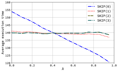
In this scenario, we run the simulation by using multiple random values of $\lambda_{i}$ , one for each classifier of the cascade. We explored how the average execution time changes when the number of classifiers increases. The other parameters of the simulation are identical to the case in the previous Section 6.2.1.

The results are displayed in Figure 7. Also in the multiple lambda case, OPT-ALG outperforms all the other approaches. In particular, the reduction in the execution time of OPT-ALG is up to $19.7\%$ compared to FIRST (average $16.6\%$ ), up to $10.1\%$ compared to BOUNDARY (average $8.2\%$ ), and up to $10.7\%$ compared to SKIP (average $9.0\%$ ).

7 A Further Generalization: Markov Processes

The $\lambda$ parameter of IDK cascades is intended to model, and thereby exploit, the temporal dependence amongst inputs in a time-series input stream. Another factor that could potentially be exploited to further speed up the average classification duration is performance correlation across the different IDK classifiers. Some performance correlation across different ML models, whereby different models produce similar results on certain kinds of data, is often due to factors like training set similarity (where models learn from nearly identical data distributions), and data structure (such as spatial or temporal patterns), which guides models to rely on the same prominent features. Additionally, model capacity and complexity, shared optimization techniques and loss functions, and regularization practices (like early stopping) can lead models to converge on similar solutions. Data preprocessing consistency and starting from the same pretrained models also align performance, as do similar bias-variance trade-offs that suit a dataset’s complexity. Together, these factors encourage different models to learn, generalize, and perform in similar ways, resulting in natural performance correlation across machine learning algorithms.

We conjecture that a Markov Process is well suited for representing both the performance correlation of models and the temporal inter-input dependence that tends to be present in the data-streams generated by CPS perception tasks. In future work, we intend to study the capabilities and limits of modeling both temporal dependencies and classifier correlations via Markov Processes; here we provide a brief overview presenting the essential idea.

A Markov Process is a stochastic process describing a sequence of possible events in which the probability of each event depends only on the state attained in the previous event. For both model correlation and inter-input temporal dependence, we can consider this state to be the identity of the boundary classifier (i.e., the least powerful classifier in the contained collection of classifiers that is able to successfully identify the current input). We can then have an $(N\times N)$ transition matrix $\Psi$ describe the probabilities of moving from one state to another for successive inputs. Specifically, in a transition matrix, each entry $\Psi_{ij}$ , ( $0\leq\Psi_{ij}\leq 1$ ), represents the probability of transitioning from $K_{i}$ being the boundary classifier for one input to $K_{j}$ being the boundary classifier for the subsequent input. The sum of the probabilities $\sum_{j}\Psi_{ij}=1$ in each row $(i)$ is 1, as they represent the total probability of moving from a particular state to any other state.

In this general formulation as a Markov Process, the single-parameter model and our generalization in Section 5.1 become special cases where state transition probabilities are correlated. When moving from the single-parameter model to the one with $N$ parameters, one needs to learn more information during runtime via on-line learning. This problem is further exacerbated if the Markov Process model is used: $(N\times N)$ different parameter values must now be learned. While this can be accomplished by directly applying the Maximum Likelihood Estimation (MLE) techniques used by Agrawal et al. [2], learning more parameter values at adequately high confidence levels requires a lot more runtime observations since a lot more information is sought to be learned.

8 Conclusions

The accurate and rapid classification of streams of inputs that are captured by sensors is an essential enabler for perception for autonomous CPS’s. In this paper, we focused on how to better leverage temporal dependencies in input streams to accelerate classification without sacrificing accuracy when using IDK cascades. A key insight was that simply starting classification from a later classifier in the cascade is suboptimal; improvements can be achieved by selectively skipping classifiers altogether. Realizing this required a technical breakthrough: we developed a linear-time cascade synthesis algorithm, significantly faster than the state-of-the-art algorithm, enabling dynamic restructuring of cascades at runtime. We also introduced a more refined temporal dependence model, assigning individual parameters to each classifier rather than a single global parameter. This improved modeling accuracy and further reduced classification latency. Experiments on synthetic datasets confirmed the performance gains of our approach. Finally, we proposed a generalized modeling framework based on Markov Processes to jointly capture temporal dependencies and classifier correlations, showing our earlier models as special cases. We leave deeper exploration of this framework to future work.

References

[1] Tarek Abdelzaher, Kunal Agrawal, Sanjoy Baruah, Alan Burns, Robert I. Davis, Zhishan Guo, and Yigong Hu. Scheduling IDK classifiers with arbitrary dependences to minimize the expected time to successful classification. Real-Time Systems, March 2023. doi:10.1007/s11241-023-09395-0.
[2] Kunal Agrawal, Sanjoy Baruah, Alan Burns, and Jinhao Zhao. IDK cascades for time-series input streams. In Proceedings of the IEEE Real-Time Systems Symposium (RTSS), York, UK, 2024. IEEE Computer Society Press.
[3] Sanjoy Baruah, Iain Bate, Alan Burns, and Robert Davis. Optimal synthesis of fault-tolerant IDK cascades for real-time classification. In Proceedings of the 30th IEEE Real-Time and Embedded Technology and Applications Symposium (RTAS 2024). IEEE, 2024. doi:10.1109/RTAS61025.2024.00011.
[4] Sanjoy Baruah, Alan Burns, Robert Davis, and Yue Wu. Optimally ordering IDK classifiers subject to deadlines. Real Time Syst., 2022. doi:10.1007/s11241-022-09383-w.
[5] Sanjoy Baruah, Alan Burns, and Robert I. Davis. Optimal synthesis of robust IDK classifier cascades. In Claire Pagetti and Alessandro Biondi, editors, 2023 International Conference on Embedded Software, EMSOFT 2023, Hamburg, Germany, September 2023. ACM, 2023. doi:10.1145/3609129.
[6] Sanjoy Baruah, Alan Burns, and Yue Wu. Optimal synthesis of IDK-cascades. In Proceedings of the Twenty-Ninth International Conference on Real-Time and Network Systems, RTNS ’21, New York, NY, USA, 2021. ACM. doi:10.1145/3453417.3453425.
[7] Thomas H. Cormen, Charles E. Leiserson, Ronald L. Rivest, and Clifford Stein. Introduction to Algorithms, 3rd Edition. MIT Press, 2009.
[8] Yizeng Han, Gao Huang, Shiji Song, Le Yang, Honghui Wang, and Yulin Wang. Dynamic neural networks: A survey. IEEE transactions on pattern analysis and machine intelligence, 44(11):7436–7456, 2021. doi:10.1109/TPAMI.2021.3117837.
[9] Yigong Hu, Shengzhong Liu, Tarek Abdelzaher, Maggie Wigness, and Philip David. On exploring image resizing for optimizing criticality-based machine perception. In 2021 IEEE 27th International Conference on Embedded and Real-Time Computing Systems and Applications (RTCSA), pages 169–178, 2021. doi:10.1109/RTCSA52859.2021.00027.
[10] Metod Jazbec, James Allingham, Dan Zhang, and Eric Nalisnick. Towards anytime classification in early-exit architectures by enforcing conditional monotonicity. Advances in Neural Information Processing Systems, 36:56138–56168, 2023.
[11] Wittawat Jitkrittum, Neha Gupta, Aditya K Menon, Harikrishna Narasimhan, Ankit Rawat, and Sanjiv Kumar. When does confidence-based cascade deferral suffice? Advances in Neural Information Processing Systems, 36:9891–9906, 2023.
[12] Yigitcan Kaya, Sanghyun Hong, and Tudor Dumitras. Shallow-deep networks: Understanding and mitigating network overthinking. In International conference on machine learning, pages 3301–3310. PMLR, 2019. URL: http://proceedings.mlr.press/v97/kaya19a.html.
[13] In Jae Myung. Tutorial on maximum likelihood estimation. Journal of Mathematical Psychology, 47(1):90–100, 2003. doi:10.1016/S0022-2496(02)00028-7.
[14] Ishrak Jahan Ratul, Zhishan Guo, and Kecheng Yang. Cascading idk classifiers to accelerate object recognition while preserving accuracy. In 49th IEEE International Conference on Computers, Software, and Applications (COMPSAC). IEEE, 2025.
[15] Xin Wang, Yujia Luo, Daniel Crankshaw, Alexey Tumanov, and Joseph E. Gonzalez. IDK cascades: Fast deep learning by learning not to overthink. CoRR, abs/1706.00885, 2017. arXiv:1706.00885.

[bib.bib1] [1] Tarek Abdelzaher, Kunal Agrawal, Sanjoy Baruah, Alan Burns, Robert I. Davis, Zhishan Guo, and Yigong Hu. Scheduling IDK classifiers with arbitrary dependences to minimize the expected time to successful classification. Real-Time Systems, March 2023. doi:10.1007/s11241-023-09395-0.

[bib.bib2] [2] Kunal Agrawal, Sanjoy Baruah, Alan Burns, and Jinhao Zhao. IDK cascades for time-series input streams. In Proceedings of the IEEE Real-Time Systems Symposium (RTSS), York, UK, 2024. IEEE Computer Society Press.

[bib.bib3] [3] Sanjoy Baruah, Iain Bate, Alan Burns, and Robert Davis. Optimal synthesis of fault-tolerant IDK cascades for real-time classification. In Proceedings of the 30th IEEE Real-Time and Embedded Technology and Applications Symposium (RTAS 2024). IEEE, 2024. doi:10.1109/RTAS61025.2024.00011.

[bib.bib4] [4] Sanjoy Baruah, Alan Burns, Robert Davis, and Yue Wu. Optimally ordering IDK classifiers subject to deadlines. Real Time Syst., 2022. doi:10.1007/s11241-022-09383-w.

[bib.bib5] [5] Sanjoy Baruah, Alan Burns, and Robert I. Davis. Optimal synthesis of robust IDK classifier cascades. In Claire Pagetti and Alessandro Biondi, editors, 2023 International Conference on Embedded Software, EMSOFT 2023, Hamburg, Germany, September 2023. ACM, 2023. doi:10.1145/3609129.

[bib.bib6] [6] Sanjoy Baruah, Alan Burns, and Yue Wu. Optimal synthesis of IDK-cascades. In Proceedings of the Twenty-Ninth International Conference on Real-Time and Network Systems, RTNS ’21, New York, NY, USA, 2021. ACM. doi:10.1145/3453417.3453425.

[bib.bib7] [7] Thomas H. Cormen, Charles E. Leiserson, Ronald L. Rivest, and Clifford Stein. Introduction to Algorithms, 3rd Edition. MIT Press, 2009.

[bib.bib8] [8] Yizeng Han, Gao Huang, Shiji Song, Le Yang, Honghui Wang, and Yulin Wang. Dynamic neural networks: A survey. IEEE transactions on pattern analysis and machine intelligence, 44(11):7436–7456, 2021. doi:10.1109/TPAMI.2021.3117837.

[bib.bib9] [9] Yigong Hu, Shengzhong Liu, Tarek Abdelzaher, Maggie Wigness, and Philip David. On exploring image resizing for optimizing criticality-based machine perception. In 2021 IEEE 27th International Conference on Embedded and Real-Time Computing Systems and Applications (RTCSA), pages 169–178, 2021. doi:10.1109/RTCSA52859.2021.00027.

[bib.bib10] [10] Metod Jazbec, James Allingham, Dan Zhang, and Eric Nalisnick. Towards anytime classification in early-exit architectures by enforcing conditional monotonicity. Advances in Neural Information Processing Systems, 36:56138–56168, 2023.

[bib.bib11] [11] Wittawat Jitkrittum, Neha Gupta, Aditya K Menon, Harikrishna Narasimhan, Ankit Rawat, and Sanjiv Kumar. When does confidence-based cascade deferral suffice? Advances in Neural Information Processing Systems, 36:9891–9906, 2023.

[bib.bib12] [12] Yigitcan Kaya, Sanghyun Hong, and Tudor Dumitras. Shallow-deep networks: Understanding and mitigating network overthinking. In International conference on machine learning, pages 3301–3310. PMLR, 2019. URL: http://proceedings.mlr.press/v97/kaya19a.html.

[bib.bib13] [13] In Jae Myung. Tutorial on maximum likelihood estimation. Journal of Mathematical Psychology, 47(1):90–100, 2003. doi:10.1016/S0022-2496(02)00028-7.

[bib.bib14] [14] Ishrak Jahan Ratul, Zhishan Guo, and Kecheng Yang. Cascading idk classifiers to accelerate object recognition while preserving accuracy. In 49th IEEE International Conference on Computers, Software, and Applications (COMPSAC). IEEE, 2025.

[bib.bib15] [15] Xin Wang, Yujia Luo, Daniel Crankshaw, Alexey Tumanov, and Joseph E. Gonzalez. IDK cascades: Fast deep learning by learning not to overthink. CoRR, abs/1706.00885, 2017. arXiv:1706.00885.

			$\displaystyle C_{1}+(1-\widehat{P_{1}})\times C_{2}+(1-\widehat{P_{2}})\times C% _{3}+(1-\widehat{P_{3}})\times C_{4}$
		$\displaystyle=$	$\displaystyle 1+0.975\times 11+0.95\times 100+0.025\times 200=\bm{111.725}$

			$\displaystyle C_{2}+(1-\widehat{P_{2}})\times C_{3}+(1-\widehat{P_{3}})\times C% _{4}$
		$\displaystyle=$	$\displaystyle 11+0.95\times 100+0.025\times 200=\bm{111.0}$

	$\displaystyle f_{j}$	$\displaystyle=$	$\displaystyle\min_{h<j}\left\{f_{h}+(1-P_{h})\cdot C_{j}\right\}$
	$\displaystyle\mbox{and\leavevmode\nobreak\ }f_{j+1}$	$\displaystyle=$	$\displaystyle\min_{h\leq j}\left\{f_{h}+(1-P_{h})\cdot C_{j+1}\right\}$

Faster Classification of Time-Series Input Streams

Abstract

Keywords and phrases:

Funding:

Copyright and License:

2012 ACM Subject Classification:

Supplementary Material:

DOI:

Supplementary Material:

Event:

Editors:

Series and Publisher:

1 Introduction

Temporal dependences in input streams.

This work.

Organization.

2 A Real-Time Model and Practical Considerations for IDK Cascades

Practical Considerations for IDK Cascades.

3 Temporal Dependences in Time-Series Input Streams

Definition 1 (dependence parameter λ).

Some Notations.

Problem Considered.

3.1 The Current State-of-the-art Classification Algorithm [2]

3.2 Can the Skip Factor Approach be Improved?

Example 2.

Our Proposed Approach.

4 A Linear-Time Cascade-Synthesis Algorithm

4.1 The Current State-of-the-art Cascade-Synthesis Algorithm [4]

Definition 3 (optimal sub-sequence Si; optimal expected duration fi).

4.2 Our New And Improved Algorithm

Lemma 4.

Proof.

Example 5.

Lemma 6.

Proof.

Lemma 7.

Proof.

5 Runtime Classification

5.1 Generalizing the Definition of Temporal Independence

Determining the 𝝀𝒌 values.

6 Experimental Evaluation

Workload generation.

6.1 Evaluating Efficiency of the Cascade-Synthesis Algorithm of Section 4

6.2 Evaluating Effectiveness of the Runtime Classification Algorithm

6.2.1 Single lambda for all classifiers

6.2.2 Multiple lambda case

7 A Further Generalization: Markov Processes

8 Conclusions

References

Definition 1 (dependence parameter $\lambda$ ).

Definition 3 (optimal sub-sequence $S_{i}$ ; optimal expected duration $f_{i}$ ).

Determining the $\lambda_{k}$ values.