Task-To-Processor Assignment for Real-Time Mixed-Critical Networked Systems Using Inductive Logic Programming

Gualtieri, Marcus; Juette, Christian; Dasari, Dakshina

doi:10.4230/LIPIcs.ECRTS.2025.14

Task-To-Processor Assignment for Real-Time Mixed-Critical Networked Systems Using
Inductive Logic Programming

Marcus Gualtieri

Robert Bosch LLC, Corporate Research, Sunnyvale, CA, USA Christian Juette

Robert Bosch LLC, Corporate Research, Sunnyvale, CA, USA Dakshina Dasari

Robert Bosch GmbH, Corporate Research, Renningen, Germany

Abstract

Task-to-processor assignment is an essential aspect of configuring real-time, distributed systems, since an improper assignment can adversely affect latency. Model-based, heuristic, and data-driven approaches have been proposed to solve the task-to-processor assignment problem. However, model-based and heuristic approaches require revision if the system changes, and data-driven approaches require training on a lot of data and setting nonintuitive hyper-parameters.

We explore a hybrid approach which takes both a system description and data: we use inductive logic programming in an active learning algorithm to search for assignments which satisfy a real-time requirement. By using both domain knowledge and data, the system finds solutions quickly, and changes are not required when using the tool on different systems. Furthermore, the output is a human-readable description of a set of predicted satisfactory assignments. Readable solution sets are useful for analyzing the system, since we can easily compare solution sets across different setups.

We evaluate our approach on real systems with mixed-critical network flows. We show that task-to-processor assignment can significantly influence latency by comparing optimal fixed assignments to the default Linux scheduler. We show that our approach finds assignments that are within 10% of optimal with up to $10\times$ fewer system tests, compared to random search. Our algorithm also performs favorably to load balancing and neural network baselines.

Keywords and phrases:

Real-Time Distributed Systems, Auto-Configuration, Task-to-Processor Mapping, Inductive Logic Programming, Active Learning

Copyright and License:

2012 ACM Subject Classification:

Computer systems organization

\rightarrow

Real-time systems ; Computer systems organization

\rightarrow

Embedded systems ; Networks

\rightarrow

End nodes

Acknowledgements:

We are grateful to Liu Ren and Philip Mundhenk, for supporting this project, Michael Wang, for discussing this paper, to Andrew Cropper, for answering questions about running Popper, and to the anonymous reviewers, for giving suggestions which improved the paper.

DOI:

10.4230/LIPIcs.ECRTS.2025.14

Event:

37th Euromicro Conference on Real-Time Systems (ECRTS 2025)

Editors:

Renato Mancuso

Series and Publisher:

Leibniz International Proceedings in Informatics, Schloss Dagstuhl – Leibniz-Zentrum für Informatik

1 Introduction

Real-time, distributed applications with mixed-critical traffic appear in automobiles and automated factories [19, 2]. For example, vehicles with a zonal architecture have networks sharing data streams with different priorities [19]. Configuring such systems to satisfy real-time requirements typically involves significant effort. This is because the application software is complex and evolving; there are countless network, device, and operating system (OS) parameters to tune; and validating configurations requires real-world testing. In this paper, we focus on a small part of the auto-configuration problem – task-to-processor assignment. Task-to-processor assignment is a beneficial starting point because an improper assignment can lead to high latency, and, with networked systems, it is not always clear what work can or should be assigned to processors interrupted by the network (Section 4). Hence there is a need for mechanisms to automatically determine this assignment.

Early research in task-to-processor assignment employed model-based approaches, where assignments are optimized on a system model rather than on the real system [3, 17]. This approach leverages domain knowledge to efficiently identify satisfactory assignments. However, any change to the system necessitates an update to the model, and this approach performs poorly when the model cannot capture the complexity of the real system. In response, heuristic-based algorithms were proposed, where assignments are optimized on the real system, and the search is guided by heuristics [12, 10]. While heuristics are a way to include domain knowledge, the heuristics may not generalize to new setups. Data-driven approaches, which learn assignment policies from examples, are more flexible than model-based and heuristic approaches [22]. Nonetheless, data-driven approaches typically require a lot of training data, time, and hyper-parameter tuning.

In this paper, we explore a hybrid approach, which requires domain knowledge and data. In particular, we use a machine learning method called inductive logic programming (ILP) in an active learning framework, where domain knowledge is provided as a set of readable, logical expressions, and the learned policies are also logical expressions. Our tool iteratively queries an assignment policy to guide the search and updates the learned policy after every system test. Compared to model-based approaches, our approach is more flexible, i.e., it works across different application loads and hardware setups. Compared to approaches with fixed search heuristics, our approach adjusts the search strategy based on experience. Compared to data-driven approaches, our approach more easily incorporates domain knowledge (i.e., logical expressions versus hyper-parameters), requires less data [8], and has more interpretable solutions (i.e., logical expressions versus neural network weights).

We investigate task-to-processor assignment in the context of a real-time, networked system, featuring both critical (i.e., latency constrained) and background (i.e., unconstrained) tasks. This is an ideal scenario for combining domain knowledge with data because solutions depend on both known and unknown aspects of the system. E.g., we found that when one or two processors are regularly interrupted by network traffic, with some hardware setups it is best to keep tasks off of the interrupted processors, but with other hardware setups it is best to keep tasks on the interrupted processors (Section 4.4). We know that “processors $x$ and $y$ are interrupted by the network” is relevant information (the domain knowledge), but we do not know exactly when interrupted processors should be assigned tasks (the data to be collected).

We propose two algorithms for the task-to-processor assignment problem. The first, called SMAL-ILP, requires some domain knowledge, represented as a logic program, and iteratively updates its heuristic until a satisfying assignment is found. The second, SMAL-NS-ILP, is similar to the first, but additionally uses a policy learned from a similar system to further narrow the search. We compare SMAL-ILP and SMAL-NS-ILP to four baselines: random assignment, load balancing, and two neural-network-based approaches. We find that, across 12 different hardware and application setups, SMAL-ILP requires fewer systems tests on average than the three baselines without pretrained policies, and SMAL-NS-ILP, and its neural network counterpart, SMAL-NS-NN, perform best.

Contribution.

Our contribution includes:

$\blacksquare$

Validating the problem of task-to-processor assignment for mixed-critical networked systems, by experimentally demonstrating: (1) a significant difference in latency with the default Linux scheduler versus an optimal assignment and (2) a dependence of the optimal task-to-processor assignment on hardware and system load (Section 4);
$\blacksquare$

Proposing two algorithms for finding satisfactory task-to-processor assignments, both of which rely on human-readable domain knowledge and data to produce human-readable assignment policies (Section 5); and
$\blacksquare$

Experimentally demonstrating that both algorithms require fewer system tests on average compared to three of the four baselines.

Terminology.

We explain the terminology used in this paper. A task is a computer program executing in response to messages or periodically on a timer. A processor is a programmable device of any kind for executing tasks. A logical processor (LP) is the most basic processor on a host, a core has one or more LPs, due to hyper-threading, and a CPU has one or more cores. An assignment is a mapping from tasks to processors. A policy is a set of assignments which are presumed to satisfy a real-time constraint.

2 Related Work

We examine earlier approaches to the task-to-processor assignment problem, especially those which study the problem in the context of real-time systems and networked systems. Also, we place our proposed algorithms in the context of existing algorithms, i.e., we classify our proposed algorithms as active learning algorithms.

Task-to-processor assignment.

Early work on the task-to-processor assignment problem assumes an analytical model of the system is given [3, 17]. While we do assume something about the system is known, because our system learns, not every important aspect needs to be described. Gandham and Alapati propose a task-to-processor assignment heuristic, where threads are assigned to processors in a round-robin fashion [10]. This is similar to the maximum entropy baseline we compare our algorithms to, which does not perform well in our experiments. Tao et al. propose a reinforcement learning (RL) agent for assigning virtual machines to a group of processors [22]. However, thousands of interactions with the system (i.e. “episodes”) are required to train the RL agent. Chen and John use fuzzy logic to infer the “suitability” of a task-to-processor assignment, considering that processors are heterogeneous [6]. As with our approach, part of their domain knowledge is represented as a set of logical expressions. However, they also require suitability scoring functions for instruction width, branch predictor size, and cache size. Our method does not rely on heuristic scoring functions: instead, it searches for assignment policies consistent with both background facts and data from system tests.

Task-to-processor assignment for real-time systems.

Several works in the real-time community have explored the task-to-processor assignment problem, focusing on different optimization goals and employing diverse mapping techniques. For example, Cruz et al. [9] proposed EagerMap, a communication-aware greedy clustering algorithm that hierarchically groups communicating tasks to reduce inter-task communication cost by mapping them to nearby cores in the network topology. Manolache et al. [17] tackled mapping and priority assignment jointly for soft real-time systems, introducing a probabilistic schedulability-driven heuristic that iteratively adjusts the task assignment to meet system-level deadline-miss ratio constraints. In the context of heterogeneous architectures, Li et al. [16] developed a heterogeneity-aware task mapping algorithm that considers execution rate disparities between CPU and GPU units to optimize for minimal overall completion time. Automotive applications are addressed by Panić et al. [18], where the RunPar algorithm exploits intra-task runnable parallelism by statically distributing fine-grained runnables across multicore platforms, while preserving dependency and activation constraints to worst-case execution time reductions. Our work is orthogonal to the above approaches, as it employs a fundamentally different methodology – inductive logic programming – and specifically addresses the challenges of mixed-criticality network flows by accounting for the load introduced by network interrupt handling.

Task-to-processor assignment for networked systems.

Salehi et al. explore different (but not mutually exclusive) types of network processing processor affinity: code affinity (select the processor which most recently touched the required protocol code), thread stack affinity (pin protocol processing threads to processors), stream affinity (pin streams to processors), and free memory affinity (pin memory pools to processors for dynamically allocated protocol structures) [21]. While Salehi et al. get deep into the OS’s network stack, our focus is at a higher level, i.e., affinity of application tasks. Hanford et al. showed that network interrupt and TCP processing affinity affects throughput [11]. With their Sandy Bridge CPUs and Mellanox ConnectX-3 NICs, it is best to assign application and TCP processing to the same CPU but a different core. We go a step further, and show that this conclusion is hardware and application dependent. Huang and Tsai propose a tool, called qcAffin, for assigning network interrupts and OS network processing threads to processors [12]. Their tool makes the assignment hierarchically through the memory structure, first assigning the task to a CPU, then to a cache domain, then to a core. Their algorithm makes the assignment based on a cost function which is made up of several heuristics, one of which attempts to balance the number of interrupts processors receive. Rather than relying on fixed heuristics, our approach adapts the search strategy as the system is evaluated. However, Huang and Tsai make use of additional information to make assignment decisions, specifically system counters, which our implementation currently does not do (a limitation of our implementation).

Active learning.

Our proposed algorithms, SMAL-ILP and SMAL-NS-ILP, can be considered active learning (AL) algorithms. The goal of AL is to learn a function with low generalization error with few labeled examples: examples are selected judiciously, since labeling is expensive [23]. In our case, we seek a task-to-processor assignment which satisfies a latency requirement with as few system tests as possible. Thus, unlike AL, learning a function with low generalization error is not our end goal. However, SMAL-ILP is an instance of what Tharwat and Schenck call “AL with Optimization” [23]. AL with optimization means a surrogate model is iteratively trained on the available, labeled examples and optimized for selecting the next example to test on the real system. We call this pattern “surrogate model active learning” (SMAL).

Our proposed algorithm is similar to the Robot Scientist, which also has a SMAL-type algorithm where the surrogate model is an ILP [4, 14, 13]. However, there are a couple of notable differences. First, the Robot Scientist explicitly considers the cost of experiments, whereas, for us, all experiments (i.e., system tests) have the same cost (a limitation of our approach). Second, the Robot Scientist, during the ILP solving step, needs to assign a probability to every possible solution, whereas our approach only uses the solution returned by the ILP solver. If the solution space is large, assigning a probability to every possible solution will not be feasible. Furthermore, since we only care about the solution returned by the ILP solver, we can treat the solver as a black-box, and use whichever solver is most efficient, without regard to the solutions visited by the solver.

The SMAL approach also appears in the systems auto-configuration literature. Bao et al. use random forests as the surrogate model for auto-configuring multiple Apache Kafka parameters [1]. We compare SMAL-ILP and SMAL-NS-ILP to two SMAL approaches where the surrogate model is a neural network.

Differentiation.

The main difference of our approach versus other task-to-processor assignment approaches, is that domain knowledge is represented as a set of logical facts, rather than as an analytical model or as heuristics. This way, the provided domain knowledge and resulting solutions are human-readable. Furthermore, the solutions are learned based on data from testing the system. This way, the provided domain knowledge can be valid across different setups. Our algorithm is similar to that of the Robot Scientist, but the application domain is computer systems rather than biological systems.

3 The Task-to-Processor Assignment Problem

Table 1: Notation that appears repeatedly in this paper.

Symbol	Description
$m$	The number of tasks in the system.
$n$	The number of processors in the system.
$a$	A task-to-processor assignment.
$\pi$	A task-to-processor assignment policy – a set of assignments.
$l$	A vector of all job latencies for every task for a given system execution.
$S$	The system: an (unknown) function mapping assignments to job latencies.
$f$	A statistic over latencies; usually, the 99.9th percentile latency of a particular task.
$B$	Background domain knowledge.
$d$	A deadline: assignments must satisfy $f(S(a))\leq d$ .

We explain the problem addressed by our algorithm. Let $T=\left\{1,\dots,m\right\}$ be a set of periodic tasks. Each task $\tau_{i}\in T$ executes $N_{i}$ times, where each execution is called a job $J_{i,j}=\langle i,j\rangle$ , for $j\in 1,\dots,N_{i}$ . Each job $J_{i,j}$ has a start time $t_{i,j}^{\textit{start}}\in\mathbb{R}_{+}$ and an end time $t_{i,j}^{\textit{end}}>t_{i,j}^{\textit{start}}$ . The latency of job $J_{i,j}$ is $l_{i,j}=t_{i,j}^{\textit{end}}-t_{i,j}^{\textit{start}}$ . Let $P=\left\{1,\dots,n\right\}$ be a set of processors. Let $a:T\to P$ be a task-to-processor assignment, where each task $\tau_{i}$ is assigned to a processor $p_{k}\in P$ . The system is an (unknown) function mapping assignments to latencies:

S(a)=[l_{1,1},l_{1,2},\dots,l_{m,N_{m}}]=l.

(1)

A system test is function call to $S$ . Let $f(l)$ be a function of latencies $l$ . We are interested in the latest latencies of a particular task. Specifically, we define the 99.9th percentile latency of task $\tau_{\iota}$ (assuming latencies are sorted from smallest to largest) as:

f(l)=l_{\iota,\lceil 0.999N_{\iota}\rceil},\text{where }l_{\iota,1}\leq l_{% \iota,2}\leq\dots\leq l_{\iota,N_{\iota}}.

(2)

Let $\Sigma=\left\{1,\dots,m\right\}$ be a set of streams. Each stream $\sigma_{i}\in\Sigma$ is the data transmitted by task $\tau_{i}$ . When data arrives at a host, the network interface card (NIC) interrupts a processor (i.e., the NIC stops any job currently running on the processor), and the processor reads the incoming data and copies it to the sockets of the destination tasks. Let $\bar{a}:\Sigma\to P$ be a function assigning streams to the processors they interrupt. Let $B=\left\{\bar{a}\right\}$ be the domain knowledge provided to our algorithm. We now define the problem as follows:

Definition 1.

Given a set of tasks $T$ , a set of processors $P$ , a system $S$ , background knowledge $B$ , a statistic $f$ , and a deadline $d$ , the task-to-processor assignment problem is to find an assignment $a$ where $f(S(a))\leq d$ , with minimum number of system tests.

Although the domain knowledge given to our algorithm is quite limited, it should be straightforward to include other information relevant to system performance. For instance, $B$ could include a description of a host’s cache structure, which is known to be important for network-intensive applications [15, 12]. Other relevant information includes data dependencies between tasks, which streams share network links, the priority of streams, and the priority of tasks.

4 Experiments to Motivate the Problem

We motivate the need for a task-to-processor assignment tool for mixed-critical distributed systems with real-world experiments. We describe an example mixed-critical distributed system (Section 4.1). We show that the 99.9th percentile latency can be much higher with the default Linux scheduler compared to the optimal, fixed assignment (Section 4.3), so a significant performance gain is possible with a different tool. We show that the optimal task-to-processor assignment is hardware and application dependent (Sections 4.4 and 4.5), so different task-to-processor assignment policies are needed for different scenarios.

4.1 An Example Mixed-Critical Distributed System

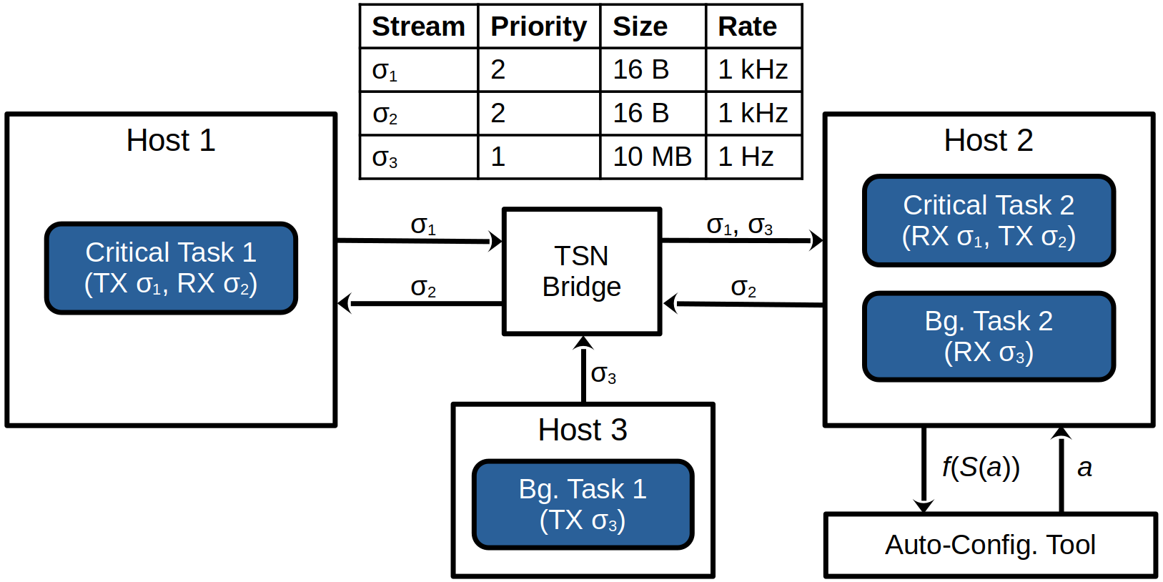
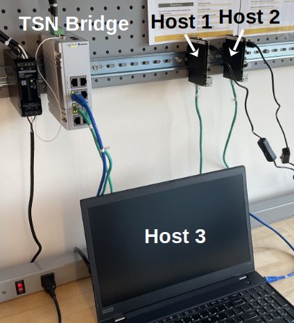
Refer to caption — Figure 1: The system used in our experiments. Host 1 sends critical messages to Host 2 at 1 kHz (stream $\sigma_{1}$ ). Host 2 replies to Host 1 as soon as possible (stream $\sigma_{2}$ ). Meanwhile, Host 3 sends large, non-critical “background” messages to Host 2 every 1 second. Critical and background traffic share the network and Host 2’s CPU.

We evaluate our ideas on the mixed-critical distributed system depicted in Figure 1. The system consists of critical tasks – tasks which must be completed before a deadline – and background tasks – tasks which are completed with best effort. Critical tasks share resources (e.g., network links and CPUs) with background tasks. Mixed-critical distributed systems like this appear in practice, e.g., in factory automation where control messages share traffic with diagnostic messages [2] or in automobiles with zonal computing architectures [19].

In this system (Figure 1), we are interested in the 99.9th percentile latency of Critical Task 1. A job of Critical Task 1 is initiated with a timer event. A job of Critical Task 1 completes as soon as a (single-frame) message from stream $\sigma_{2}$ is taken from the socket and is deserialized. Critical Task 1 could be, e.g., a robot’s control loop, where sensor data is sent to a controller, and the controller replies with an action. Background messages could be, e.g., model updates to the robot’s controller. We find that the task-to-processor assignment for tasks running on Host 2 significantly impacts the latency of Critical Task 1. Thus, we explore optimizing the task-to-processor assignment for the tasks running on Host 2.

Table 2: Description of the scenarios in Dataset 1.

Scenario	CPU	NIC	Critical Tasks	Bg. Tasks	Accesses
S1	Arm Cortex A72	Raspberry Pi 4	1	1	0
S2	Arm Cortex A72	Raspberry Pi 4	1	1	32k
S3	Arm Cortex A72	Raspberry Pi 4	2	1	0
S4	Arm Cortex A72	Raspberry Pi 4	2	2	0
S5	Intel Xeon ES1270	Realtek RTL8125B	1	1	0
S6	Intel Xeon ES1270	Intel I226-T1	1	1	0

Table 3: Description of the scenarios in Dataset 2.

Scenario	CPU	NIC	Critical Tasks	Bg. Tasks	Accesses
S1	Arm Cortex A76	Raspberry Pi 5	1	1	0
S2	Arm Cortex A76	Raspberry Pi 5	1	1	32k
S3	Arm Cortex A76	Raspberry Pi 5	2	1	0
S4	Arm Cortex A76	Raspberry Pi 5	2	2	0
S5	Intel Xeon ES1270	Intel I219-LM	1	1	0
S6	Intel Xeon ES1270	TP-Link TG3468	1	1	0

To see how well our algorithms generalize, we test various instantiations of the mixed-critical distributed system shown in Figure 1. The variations we test are described in Tables 2 and 3. We test three CPUs, including two 4-core Arm CPUs and one 4-core Intel CPU (which has 8 LPs, due to hyper-threading). We test six different network interface cards (NICs), one of which has multiple receive queues (the I226-T1). We test adding an identical critical and/or background task to Host 2. Finally, we test different memory access loads, to influence the contents of the CPU cache. “Accesses” refers to the number of 1 byte reads from a 256 KiB region of memory, where the read location is sampled uniformly at random, for each message received, for each task on Host 2.

Some additional details. The LP interrupted by the network is always $p_{0}$ , except when the Intel I226-T1 NIC is used, where background traffic interrupts $p_{0}$ and critical traffic interrupts $p_{1}$ . Each of the 4 cores of the Intel Xeon have two LPs: $(p_{0},p_{4})$ , $(p_{1},p_{5})$ , $(p_{2},p_{6})$ , and $(p_{3},p_{7})$ . Dynamic voltage and frequency scaling was disabled on all hosts. All hosts run Ubuntu 22.04 with the PREEMPT_RT kernel patch applied. For networking, we use a minimal, custom protocol to control the priority of frames on network and end devices. The custom protocol is built directly on top of Ethernet where streams are identified by VLAN ID, stream priority is identified by the VLAN PCP field, and messages are sent with best effort reliability (i.e., no resend). Critical tasks have real-time priority (SCHED_RR and priority 98) and background tasks have the default priority.

4.2 Data Collection Procedure

Data for each scenario in Tables 2 and 3 are collected by testing every possible task-to-processor assignment (i.e., all $n^{m}$ assignments). We record all job latencies for Critical Task 1 during a period of 30 seconds (following a 3-second warm-up period). From these latencies, the 99.9th percentile latency is computed (Equation 2).

4.3 Optimal Assignment Versus Default Linux

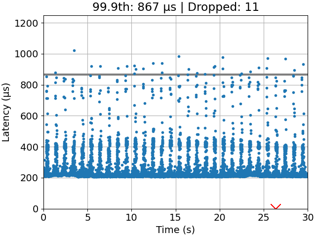
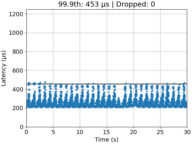
We find that an optimal¹¹1An optimal task-to-processor assignment is a task-to-processor assignment with minimum 99.9th percentile latency, i.e., $a^{\star}=\operatorname*{argmin}_{a}f(S(a))$ . task-to-processor assignment can indeed perform significantly better than the default Linux scheduler, called the Completely Fair Scheduler (CFS) [5]. A comparison is shown in Figure 2 with time-series plots. Gandham and Alapati came to a similar conclusion but with a different application (common data structure operations) and performance measure (throughput) [10]. Thus, we conclude that task-to-processor assignment is still a relevant problem for latency-sensitive applications.

4.4 Hardware Dependence

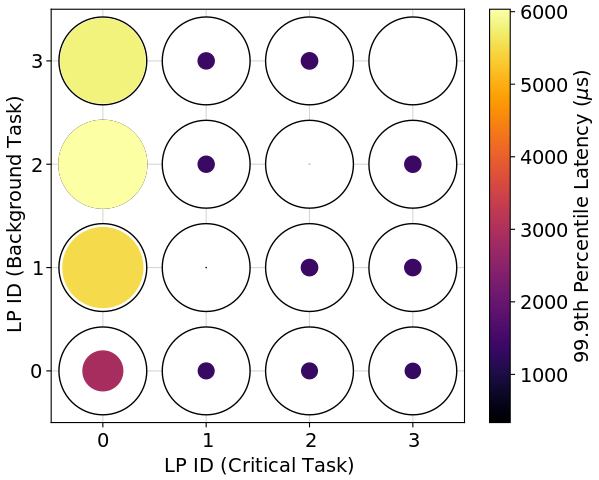
We find the best-performing task-to-processor assignments (in a 99.9th percentile sense) vary by hardware setup. Figure 3 shows the performance of different assignments for different hardware setups. For the Raspberry Pi 4, the best assignments have the critical and background tasks sharing a logical processor (LP). For the Intel Xeon with the Realtek NIC, there are only two configurations that are far from optimal: (1) placing the critical and background tasks on the interrupted LP (LP 0) or (2) placing the critical task on the interrupted hyper-thread (LP 4) and the background task on the interrupted LP (LP 0). However, placing both the critical and background tasks on the interrupted hyper-thread (LP 4) is the optimal choice. For the Intel Xeon with the multi-queue NIC, it is generally better to place the critical task on the LP (or hyper-thread) interrupted by critical traffic (LP 1 or 5) and the background task on the LP (or hyper-thread) interrupted by background traffic (LP 0 or 4). However, all assignments perform well with this setup.

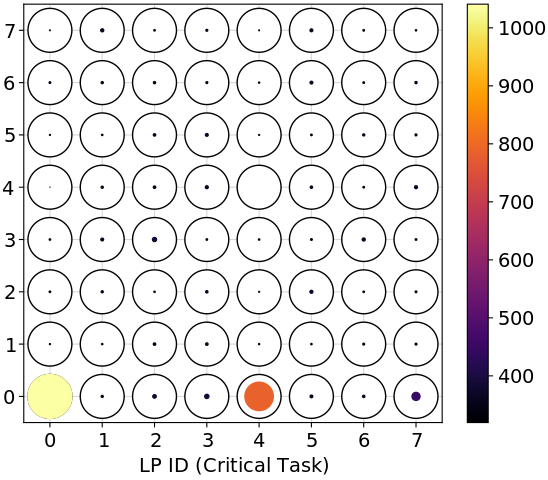
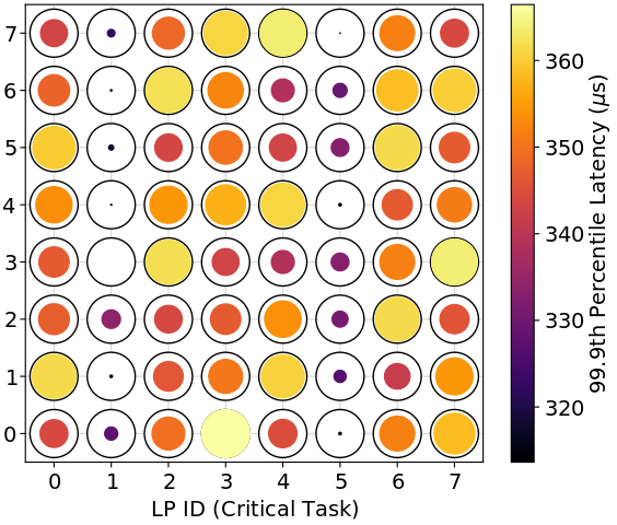
It is not surprising that different hardware setups would have different performance patterns: after all, vendors are free to implement their products in different ways. Indeed, Klug et al. also found that hardware was relevant for task-to-processor assignment, in particular, the best level of sharing of threads on a single core is different on AMD versus Intel chips [15]. Instead of designing one heuristic that works for every setup, we auto-generate simple and readable heuristics (i.e., assignment policies) for each setup.

4.5 Impact of Memory Access on Application Latency

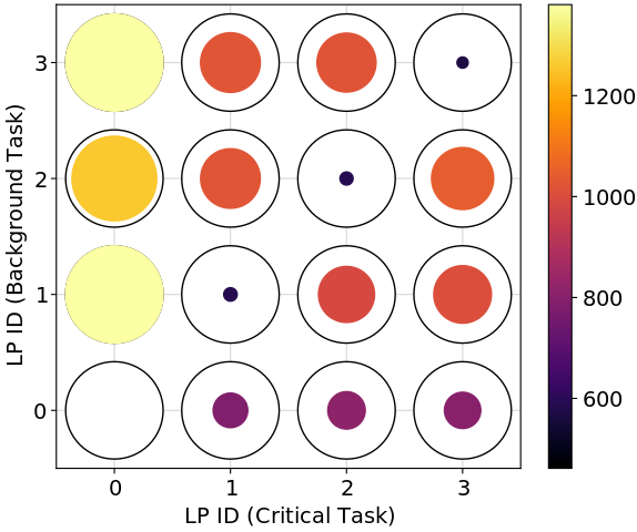
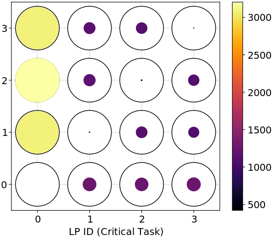
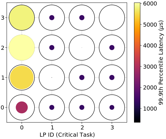
We find the best-performing task-to-processor assignments (in a 99.9th percentile sense) depend on the application’s memory access load. Figure 4 shows the performance pattern for three different loads. We see from the values in the color bar that memory accesses do severely affect latency. Furthermore, the optimal assignment shifts from placing everything on the interrupted LP (i.e., LP 0) to placing the critical and background tasks on the same LP (but not on the interrupted LP). This is presumably because the interrupted LP eventually becomes overwhelmed.

Because application load can easily change, it is useful to have a tool which automatically finds a task-to-processor assignment satisfying our timing requirements. The default Linux scheduler is not an option, since it can perform poorly compared to the optimal assignment (Section 4.3).

5 Methods

We explain how ILP can be used to address the task-to-processor assignment problem. We start by explaining how to generate an assignment policy when the 99.9th percentile latency of all assignments is known. Then, we describe two algorithms for deciding the next assignment to test, when, initially, none of the 99.9th percentile latencies are known. We end by mentioning how ILP could apply to auto-configuration in general.

5.1 Background: Inductive Logic Programming

Inductive logic programming (ILP) is an approach to machine learning [7]. The goal is, given a set of background facts (the domain knowledge) and a set of examples, generate a set of logical rules, called a hypothesis, that explains the set of examples. That is, the hypothesis should correctly classify examples not seen at the time the hypothesis was generated. Compared to other approaches to machine learning, such as neural networks, ILP uses a set of background facts, also represented by a set of logical rules, to generate hypotheses. This makes it easy to incorporate domain knowledge into the learning problem.

For instance, consider the problem of learning the concept “grandparent”.²²2This example derives from Russel and Norvig [20]. The background information (Equation 3) consists of facts about who is the mother or father of whom. For example, mother(mum, elizabeth) means, “Mum is the mother of Elizabeth.” Positive examples of grandparents, $E+$ , and negative examples, $E^{-}$ , are also given (Equation 4). Given $B$ , $E^{+}$ , and $E^{-}$ , the ILP solver Popper [8] learns the hypothesis in Equation 5.

B=\left\{\begin{array}[]{lr}\text{mother(mum, elizabeth).}\\ \text{mother(elizabeth, charles).}\\ \text{mother(diana, harry).}\\ \text{father(george, elizabeth).}\\ \text{father(philip, charles).}\\ \text{father(charles, harry).}\\ \end{array}\right\}

(3)

E^{+}=\left\{\begin{array}[]{lr}\text{grandparent(mum,charles).}\\ \text{grandparent(george,charles).}\\ \text{grandparent(elizabeth,harry).}\\ \text{grandparent(philip,harry).}\\ \end{array}\right\};E^{-}=\left\{\begin{array}[]{lr}\text{grandparent(charles,% charles).}\\ \text{grandparent(george,elizabeth).}\\ \text{grandparent(elizabeth,charles).}\\ \end{array}\right\}

(4)

H=\left\{\begin{array}[]{lr}\text{grandparent(V0, V1):- mother(V0, V2), mother% (V2, V1).}\\ \text{grandparent(V0 ,V1):- mother(V0, V2), father(V2, V1).}\\ \text{grandparent(V0 ,V1):- father(V0, V2), mother(V2, V1).}\\ \text{grandparent(V0, V1):- father(V0, V2), father(V2, V1).}\\ \end{array}\right\}

(5)

This syntax is from Prolog. “ $h\textit{:- }b_{1},\dots,b_{n}$ ” is called a clause. It is an implication: $b_{1}\land b_{2}\land\dots\land b_{n}\implies h$ . Multiple clauses with the same head, e.g., $h\textit{:- }b_{1}$ and $h\textit{:- }b_{2}$ represent an “or” relationship: $b_{1}\lor b_{2}\implies h$ . Variables start with a capital letter and are universally quantified (i.e., the clause applies to all possible groundings of the variable). Thus, the first line in Equation 5 translates to, “For all V0, V1, and V2, if V0 is the mother of V2, and V2 is the mother of V1, then V0 is a grandparent of V1.” Database semantics apply – anything that is not true given the background information and the hypothesis is assumed to be false.

A simpler hypothesis would have been generated if the concept “parent” were included in the background information. Some ILP solvers can invent predicates, like “parent”, which are not present in the background information, in order to return a simpler hypothesis [7]. This feature is called predicate invention [7]. Predicate invention is useful when some relevant background information is unknown. Also, some ILP solvers are able to find recursive hypotheses, i.e., hypotheses that contain clauses which refer to themselves. This is useful for learning computer programs. Finally, many ILP solvers can handle noise, i.e. mislabeled examples [7]. In this case, hypotheses are generated which maximize a learning performance measure, e.g., accuracy, precision, or recall.

For the experiments in this paper, predicate invention and recursion are not required. In the future, we would like to see if these features are required for more advanced auto-configuration problems. However, it is clearly important for the solver to handle noisy labels, as our labels come from experiments on a real system. The solver we use is called Popper [8].

5.2 Domain Knowledge Represented as a Logic Program

To learn hypotheses, ILP needs background information. From our data (e.g., Figure 3) and the results in [21, 11, 12], we know that, for network-intensive applications, information about which logical processors (LPs) are interrupted by the network is relevant to the task-to-processor assignment problem. Thus, the network-interrupted LPs are identified in our background information. The background information for all of our Raspberry Pi scenarios is shown in Listing 1. We define which LPs there are (0, 1, 2, and 3) and what it means for tasks to be on the same LP or on different LPs. We also indicate which LPs are interrupted by the network and which LPs are not interrupted by the network.

Listing 1: Background information used for Raspberry Pi scenarios (S1 - S4 in Tables 2 and 3).

⬇

% The logical processors (LPs) that are defined.

lp(0). lp(1). lp(2). lp(3).

% True if two tasks are on the same LP.

shares_lp(0, 0). shares_lp(1, 1). shares_lp(2, 2). shares_lp(3, 3).

% True if two tasks are on different LPs.

diff_lps(1, 0). diff_lps(2, 0). diff_lps(3, 0). diff_lps(0, 1).

diff_lps(2, 1). diff_lps(3, 1). diff_lps(0, 2). diff_lps(1, 2).

diff_lps(3, 2). diff_lps(0, 3). diff_lps(1, 3). diff_lps(2, 3).

% Indicates which LP is interrupted by the network.

on_intr_lp(0).

% Indicates which LPs are not interrupted by the network.

off_intr_lp(1). off_intr_lp(2). off_intr_lp(3).

When hyper-threads are present (scenarios S5 and S6 in Tables 2 and 3), we have two additional predicates: on_intr_ht, which indicates that an LP shares a core but is on a different hyper-thread from network interrupts, and off_intr_ht, which is the negation of on_intr_ht. When a multi-queue NIC is used (scenario S5 in Table 2), we replace on_intr_lp(0) with on_bg_intr_lp(0) and on_cr_intr_lp(1) to indicate that LP 0 is interrupted by background traffic and LP 1 is interrupted by critical traffic, and similar replacements are made for off_intr_lp, on_intr_ht, and off_intr_ht.

5.3 Labeled Task-to-Processor Assignments

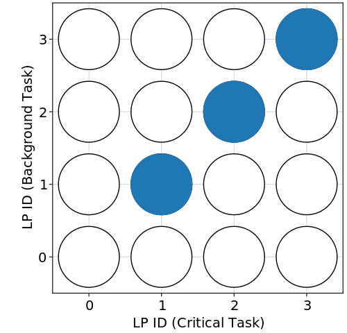
To learn hypotheses, ILP needs labeled examples. In our case, we label task-to-processor assignments according to whether or not they satisfy the real-time requirement $f(l)\leq d$ , where $f(l)$ is the 99.9th percentile latency. We choose $d$ to be within 10% of the optimal assignment, i.e., $d=1.10f(S(a^{\star}))$ . We choose a scenario-dependent $d$ rather than a fixed $d$ so that solution assignments are “nearly optimal” regardless of how performance scales with hardware capabilities. Figure 5(b) shows which assignments satisfy the requirement $f(l)\leq d$ for Dataset 1, scenario S2.

Listing 2 shows the labels in Figure 5(b) in Prolog syntax – the format required by Popper. An assignment assign(A, B) means the critical task is assigned to LP A and the background task is assigned to LP B. If there are more tasks, the predicate assign will take more arguments. pos means the assignment satisfies the real-time requirement, and neg means the assignment does not satisfy the real-time requirement.

Listing 2: Labeled assignments for scenario S2 (Table 2).

⬇

pos(assign(1,1)).pos(assign(2,2)).pos(assign(3,3)).neg(assign(0,0)).

neg(assign(0,1)).neg(assign(0,2)).neg(assign(0,3)).neg(assign(1,0)).

neg(assign(1,2)).neg(assign(1,3)).neg(assign(2,0)).neg(assign(2,1)).

neg(assign(2,3)).neg(assign(3,0)).neg(assign(3,1)).neg(assign(3,2)).

5.4 Task-to-Processor Assignment Policies

Given the background information in Listing 1 and the examples in Listing 2, the ILP solver Popper [8] generates the hypothesis in Listing 3. The hypothesis is translated, “An assignment satisfies the real-time requirement $f(l)\leq d$ if the critical and background tasks share an LP and the background task is not on the LP interrupted by the network.”

Listing 3: Hypothesis generated from the background in Listing 1 and the examples in Listing 2.

⬇

assign(V0,V1):- shares_lp(V0,V1), off_intr_lp(V1).

The hypothesis describes a set of assignments. We call a set of assignments, $\pi=\{a_{1},a_{2},\dots\}$ , a policy. Although the task-to-processor assignment problem only requires finding a single satisfying assignment, we conjecture that policies obtained inductively, with an appropriate set of background information, can guide the search for the first satisfying assignment. That is, the assignment policy should contain a larger ratio of satisfying untested assignments to untested assignments, versus the same ratio for all possible assignments.

5.5 Task-to-Processor Assignment Algorithms

We now explain two algorithms which address the task-to-processor assignment problem (Section 3). Both use background knowledge (Section 5.2), examples (Section 5.3), and policies (Section 5.4) to guide the search. The first algorithm is a surrogate model active learning (SMAL) approach [23]. The second algorithm is similar to the first, except it additionally makes use of a policy generated from data from the nearest scenario (NS) in a database. We evaluate both algorithms experimentally in Section 6.2.

5.5.1 SMAL-ILP

Algorithm 1 Surrogate model active learning (SMAL) ILP.

The idea of SMAL-ILP (Algorithm 1) is to query a working assignment policy (i.e., an ILP hypothesis) for the next assignment to test, test the assignment on the real system, update the working policy with the result, and repeat until a satisfying assignment is found. In order to generate non-trivial policies during the search process, SMAL-ILP assumes all untested configurations are positive examples and all tested configurations are negative examples.

The reason SMAL-ILP finds a solution with fewer system tests than random search is because the background information guides the search. An appropriate amount of background information results in a non-trivial hypothesis (i.e., some positive examples are labeled positive and some negative examples are labeled negative) without over-fitting (i.e., some positive examples are indeed labeled negative). If the hypothesis perfectly labels the examples, we do no better than random search, because, in this case, the predicted positives are all untested examples. The background information controls the space of admissible policies.

5.5.2 SMAL-NS-ILP

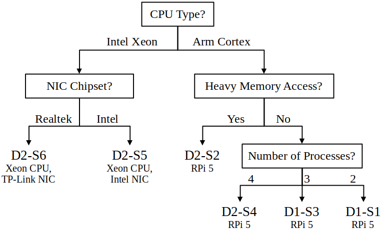
Algorithm 2 SMAL nearest scenario ILP.

SMAL-NS-ILP (Algorithm 2) builds on SMAL-ILP. The only difference is that SMAL-NS-ILP additionally relies on a policy generated from previous experience. SMAL-NS-ILP begins by querying a database of existing policies, matching the current scenario with the most similar, previous scenario. The “scenario descriptor” is, e.g., a list of key-value pairs, e.g., CPU Type = Intel, NIC Type = Multi-queue, Number of Processors = 2. The “database” could be implemented with, e.g., a decision tree, as in Figure 7. The database query returns the nearest policy, i.e., the policy generated for the scenario matching the query.

SMAL-NS-ILP then proceeds just as SMAL-ILP except: (1) we restrict positive examples to assignments in the nearest policy (unless there are none) and (2) we restrict the search to assignments in the nearest policy (unless there are none). This way, the working policy initially attempts to imitate the nearest policy but gradually evolves as new evidence comes in, again using the background domain knowledge to guide the search.

5.5.3 Analysis of SMAL-ILP

We analyze the correctness and time complexity of SMAL-ILP.³³3The analysis of SMAL-NS-ILP is similar. This section requires additional notation for this section only. We use the logic terminology from [7]. The result suggests that the algorithm may not scale well with the number of tasks. Thus, at the end of this section, we suggest approximate algorithms where iterations scale linearly in the number of tasks; although, these approximations were not required for our example scenarios.

Inputs and outputs.

$m$ is the number of tasks and $n$ is the number of processors. $B$ is the background information, i.e., a set of clauses. $E=E^{+}\cup E^{-}$ is a set of examples, i.e., the set of assign literals, each labeled pos or neg. $\mathcal{H}$ is the set of all possible hypotheses, and $H\in\mathcal{H}$ is a hypothesis, i.e., a set of clauses.

Constants.

$\alpha\in\mathbb{N_{+}}$ is the maximum arity (i.e., number of arguments) of any literal in $B$ and $H$ . $\beta\in\mathbb{N_{+}}$ is the number of predicate symbols in $B$ . $c\in\mathbb{N}_{+}$ is the maximum number of clauses in any $H$ . $C\in\mathbb{N}_{+}$ is any constant large enough to ensure the bounds are satisfied.

Assumptions on background information.

The type of background information we use for task-to-processor assignment is more limited than what is possible with ILP solvers like Popper. Specifically, we make the following simplifying assumptions on $B$ :

$\blacksquare$

$B$ is a set of ground positive literals.
$\blacksquare$

Each literal has maximum arity $\alpha$ .
$\blacksquare$

There are at most $\beta$ predicate symbols.
$\blacksquare$

A predicate symbol appears at most $n^{\alpha}$ times in $B$ .

There are at most $n^{\alpha}$ literals in $B$ with the same predicate symbol because, for each literal in $B$ : each argument is a processor ID, there are at most $n$ processor IDs, and there are at most $\alpha$ arguments. Thus, the number of literals in $B$ is related to the number of processors $n$ :

\lvert B\rvert\leq n^{\alpha}\beta

(6)

Assumptions on hypotheses.

Likewise, the type of hypotheses we use for task-to-processor assignment is more limited than what is possible with Popper. We make the following assumptions on each $H\in\mathcal{H}$ :

$\blacksquare$

$H$ is a set of at most $c$ definite clauses.
$\blacksquare$

Each head literal in $H$ is $\textit{assign}(V_{1},\dots,V_{m})$ , where $V_{1},\dots,V_{m}$ are variables.
$\blacksquare$

There are no more than $m$ body literals.
$\blacksquare$

Each body literal has maximum arity $\alpha$ .
$\blacksquare$

A variable in the body of $H$ is an element of $\{V_{1},\dots,V_{m}\}$ .
$\blacksquare$

A predicate symbol in the body of $H$ is one of the $\beta$ predicate symbols from $B$ .
$\blacksquare$

The predicate assign is not included in the body of $H$ , i.e., no recursive hypotheses.

Correctness.

Assuming the system $S$ is deterministic, SMAL-ILP is sound: if an assignment is returned, it has been tested on the system and the 99.9th percentile latency satisfies the deadline. SMAL-ILP is also complete: if no assignments satisfy the deadline, all assignments will be tested before fail is returned. So the worst-case time complexity is $O(\textit{It}\cdot n^{m})$ , where It is the time complexity per iteration.

We are only interested in the time complexity of It: assuming the system (the function $S$ ) is unknown, every complete algorithm will have time complexity $O(\textit{It}\cdot n^{m})$ .

Size of the hypothesis space.

Plugging in our assumptions into the hypothesis space size given in Cropper and Morel [8], we have:

	$\displaystyle\lvert\mathcal{H}\rvert$	$\displaystyle\leq\sum_{j=1}^{c}\binom{\sum_{i=1}^{m}\binom{\beta m^{\alpha}}{i% }}{j}$		(7)
		$\displaystyle\leq C(\beta m^{\alpha})^{mc}$		(8)

Time complexity.

Here, we provide an upper bound on the time complexity of an ILP solver, given our simplifying assumptions on $B$ and $\mathcal{H}$ , and assuming a naïve algorithm of evaluating every hypothesis on every example. Popper will not, except in trivial cases, visit each $H\in\mathcal{H}$ , since Popper prunes the hypothesis space on every failed hypothesis [7]. However, the time complexity of Popper with simplified background information and hypotheses has not been analyzed in [7]. For simplicity, we analyze the complexity of evaluating every hypothesis on every example.

To evaluate a single hypothesis for completeness and consistency with the examples and background information, we need $\leq Cm\lvert E\rvert$ computations.⁴⁴4Evaluating a hypothesis involves, for each example, (1) grounding each variable in $H$ and (2) checking if each ground body literal in $H$ is in $B$ . Step 1 requires no more than $C m$ groundings, since there are at most $\alpha cm$ variables in $H$ . Step 2 requires no more than $C m$ steps: assuming we pre-compute a hash table and a hash function for $B$ , in the worst case, each literal in $H$ requires a lookup in $B$ , and there are at most $c m$ such literals. Putting this together, evaluating a hypothesis takes at most $Cm\lvert E\rvert$ steps. Putting this together with the size of the hypothesis space, the run time of one iteration of SMAL-ILP is bounded by:

\textit{It}_{\textit{SMAL-ILP}}\leq Cm\lvert E\rvert\lvert\mathcal{H}\rvert,

(9)

Where $|E|=n^{m}$ . Unfortunately, this bound does not scale well with $m$ . However, in our experiments, this bound appears to be very loose.

Example time complexity.

In our experiments, the largest value of Equation 9 comes from scenario S4 in either Table 2 or Table 3. Here, $\alpha=2$ , $\beta=5$ , $c=6$ , $m=4$ , $n=4$ , $\lvert B\rvert\leq 80$ (Equation 6), $\lvert E\rvert=256$ , $\lvert\mathcal{H}\rvert\leq 3.0\times 10^{34}$ (Equation 7), and $\textit{It}_{\textit{SMAL-ILP}}\leq C\times 3.1\times 10^{37}$ (Equation 9). In reality, however, an iteration completes in roughly 1 second.

Suboptimal alternatives.

If the time it takes to run one iteration of SMAL-ILP becomes infeasible, limits could be imposed on $\lvert E\rvert$ and $\lvert\mathcal{H}\rvert$ . If a constant number of examples are sampled from the complete set, and a constant maximum number of hypotheses are checked by the ILP solver, the bound (Equation 9) becomes linear in $m$ . In this case, the solutions produced by the ILP solver are not guaranteed to be optimal (as defined in [8]); although, SMAL-ILP remains sound and complete. These alternatives were not required in the experiments of Section 6, where we have at most 4 tasks, but alternative methods were required in experiments with 12 tasks (Appendix C).

5.6 Summary: Example Application of the Methods

We illustrate a process for applying our methods to a new task-to-processor assignment problem (Figure 6). The first step is to determine the relevant domain knowledge for the problem, which currently requires human expertise. In our case, through experimentation, we found “the IDs of processors interrupted by the network” is relevant information (as discussed further in Appendix A). Once this is done, we describe the domain knowledge using Prolog syntax, as we do in Section 5.2 (and Appendix C). Next, the search algorithm is run, and learned policies are saved in a database to accelerate future searches.

6 Experiments

We provide examples of readable task-to-processor assignment policies learned by ILP, and we experimentally compare SMAL-ILP and SMAL-NS-ILP to four baselines.

6.1 Human-Readable Policies

Earlier (in Section 5.2), we showed an example of readable domain knowledge for learning task-to-processor assignment. Now we give examples of readable task-to-processor policies. Listing 4 shows three policies generated by Popper, where every possible assignment was evaluated and labeled. The first policy translates to, “An assignment is satisfactory if the critical task is on the interrupted LP and the background task is also on that LP.”

Listing 4: Policies generated by Popper for the three scenarios in Figure 3, given the complete dataset for those scenarios. Examples are considered positive if the 99.9th percentile latency is within 10% of optimal. V0 is the critical task and V1 is the background task.

⬇

% Policy for Raspberry Pi 4 (S1).

assign(V0,V1):- on_intr_lp(V0), shares_lp(V0,V1).

% Policy for Intel Xeon, Realtek NIC (S5).

assign(V0,V1):- on_intr_lp(V0), off_intr_lp(V1).

assign(V0,V1):- on_intr_ht(V0), off_intr_lp(V1).

assign(V0,V1):- off_intr_lp(V0), shares_lp(V0,V1).

% Policy for Intel Xeon, I226-T1 NIC (S6).

assign(V0,V1):- on_crcl_intr_lp(V0).

assign(V0,V1):- on_crcl_intr_ht(V0).

assign(V0,V1):- shares_lp(V0,V1), on_bkgd_intr_lp(V1).

assign(V0,V1):- on_bkgd_intr_ht(V0), on_crcl_intr_ht(V1).

assign(V0,V1):- on_bkgd_intr_ht(V0), on_bkgd_intr_lp(V1).

Readability enables experts to compare the task-to-processor assignment policies of different systems in a logical, symbolic way. For example, from Listing 4, we see the policies for S1 and S5 contradict each other (for S1, the background process must be on the interrupted LP, and for S5, the background process cannot be on the interrupted LP), and the policy for S6 involves different symbols (the stream interrupting the processor is relevant). From these differences, we conclude that the satisfactory task-to-processor assignment policy depends on hardware setup. Earlier we came to a similar conclusion by comparing the latency plots (Figure 3), but having a symbolic comparison adds to our confidence.

6.2 Task-to-Processor Assignment

We empirically compare six different algorithms for addressing the task-to-processor assignment problem. We find that SMAL-ILP requires fewer system tests than the non-NS baselines, and the NS approaches require the fewest. We also empirically observe that the run time of SMAL-ILP and SMAL-NS-ILP is lower than a neural network approach, and the run time scales well with $n^{m}$ , the number of possible assignments.

6.2.1 Data Collection Procedure

For each scenario in Tables 2 and 3, Datasets 1 and 2 are constructed from the 99.9th percentile latency for every possible assignment, using the procedure in Section 4.2. Dataset 2 (from the scenarios in Table 3) was not observed when we designed the background information, so Dataset 2 serves as a kind of test set, to check if our background information generalizes to a similar setup with different hardware. An assignment is considered positive if and only if it is within 10% of optimal (Section 5.3). We track the number of times each algorithm queries the dataset for the 99.9th percentile latency of an assignment.

6.2.2 Baselines

We compare our algorithms, SMAL-ILP and SMAL-NS-ILP, to four baselines:

$\blacksquare$

Random. Selects the next assignment uniformly at random without replacement. This is a strong baseline when a large proportion of the assignments is positive.
$\blacksquare$

Entropy. Distributes tasks over processors as uniformly as possible. A task-to-processor assignment can be viewed as a discrete probability distribution (Equation 10, where $\mathbb{I}$ is the indicator function). This method selects the next assignment whose associated probability distribution has maximal Shannon entropy (without replacement, and ties are broken uniformly at random). Several related works have the same goal: balance processing load [10, 12]. Load balancing makes sense for systems where processor load (and not memory access) is the most significant factor affecting latency.

$\Pr(p_{i})=\frac{1}{m}\sum_{j=1}^{m}\mathbb{I}\left(a(\tau_{j})=p_{i}\right),% \text{for }i=1,\dots,n$ (10)
$\blacksquare$

SMAL-NN. Uses a neural network as the surrogate model. SMAL-NN trains a neural network to predict the 99.9th percentile latency given the labeled examples seen so far. The next assignment is chosen to minimize predicted latency (without replacement). A properly regularized neural network should be able to accurately predict unseen latencies.
$\blacksquare$

SMAL-NS-NN. Trains a network on the nearest scenario’s complete dataset to predict 99.9th percentile latency. Uses a 2nd network, just as SMAL-NN, but with the constraint that assignments classified⁵⁵5Classification is based on the within 10% of optimal value from the nearest scenario’s dataset; whereas, testing is based on the within 10% of optimal value for the test dataset. as positive by the NS network are all evaluated first.

Some details about SMAL-NN (and SMAL-NS-NN). The neural network architecture is a fully-connected network with one hidden layer (with ReLU activations). To avoid over-fitting, we tuned hyper-parameters (the number of hidden units, weight decay, learning rate, batch size, and number of iterations) on Dataset 1 by gradually increasing regularization until the maximum %-error exceeded a threshold. We expect SMAL-NN to do well because it has some additional information SMAL-ILP does not have – the continuous latency values. However, SMAL-NN does not have the background information provided by the domain expert. To compensate, the set of policies that are considered by SMAL-NN is constrained by the tuned hyper-parameters.

6.2.3 Deciding Nearest Scenarios in SMAL-NS-ILP and SMAL-NS-NN

SMAL-NS-ILP (Algorithm 2) requires a database of policies and a procedure for identifying the “nearest scenario”. We have two policy databases: (1) a policy for each scenario in Dataset 1 (Table 2) and (2) a policy for each scenario in Dataset 2 (Table 3). We use the policies generated from Dataset 2 to evaluate SMAL-NS-ILP on Dataset 1, and we use the policies generated from Dataset 1 to evaluate SMAL-NS-ILP on Dataset 2. To match scenarios, we hand-made decision trees (Figure 7) to decide which policy from the other dataset to use.

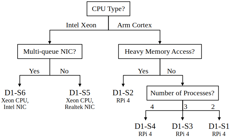
To quantify the informativeness of a nearest scenario for searching for satisfactory assignments in the test scenario, we compare the nearest scenario’s positives to the test scenario’s positives (Table 4). Since the “% NS Positives Overlap” is higher than the “% Positives” in every scenario (except Dataset 1, Scenario 6), a policy trained on a nearest scenario will generally help to speed up the search for the first satisfactory assignment. (See Appendix B for a more detailed explanation).

Table 4: % Positives: The proportion of assignments in the dataset which are “positive”, i.e., within 10% of optimal. % NS Positives Overlap: The proportion of positives in the nearest scenario which are also positive in the test scenario. For each of our scenarios, the space of possible assignments for the test scenario and for the nearest scenario are the same.

Scenario (D1 \| D2)	S1	S2	S3	S4	S5	S6	S1	S2	S3	S4	S5	S6
% Positives	6	18	9	2	50	42	25	25	29	3	67	93
% NS Positives Overlap	25	75	31	25	53	39	100	100	100	28	75	100

6.2.4 Results: Number of System Evaluations

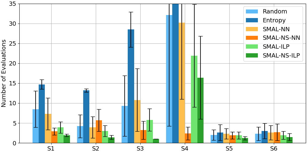
Figures 8 and 9 show how the six methods perform on the task-to-processor assignment problem on Dataset 1 and Dataset 2, respectively. Results for “Random” are computed analytically; all other results are averages (and sample standard deviations) over 30 trials.

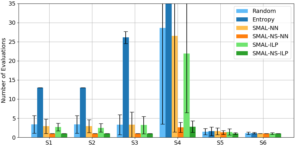
SMAL-NS-ILP performs best in 10/12 scenarios (it loses to SMAL-NS-NN in D1-S4, because its nearest policy is the empty set, and again in D2-S4, where performance is close). When there are many possible assignments but few positives, SMAL-NS-ILP can reduce the required number of evaluations substantially. (E.g., there were 2.8 evaluations for SMAL-NS-ILP and 28.6 evaluations for Random for D2-S4, where 8 of 256 assignments are positive.) SMAL-ILP generally performs better than Random; however, the difference is small when the proportion of positive assignments is 30% or more (see “% Positives” in Table 4). SMAL-NN does not clearly perform better than Random. SMAL-NS-NN generally performs better than Random (except in D1-S2, because the NS network has low precision on its training dataset, and D1-S6, because the NS positives do not overlap well with positives in the test scenario – see Table 4). Entropy performs the worst: for both instances of Scenario 4, the number of evaluations is off the chart (over 200 in each case). Entropy performs worst on the Raspberry Pi devices.

Interpretation.

We are not surprised that SMAL-ILP, SMAL-NS-ILP, and SMAL-NS-NN perform better than Random: these approaches utilize domain knowledge and previously learned policies to guide the search. However, it is surprising that Entropy performs worse than Random, especially since load balancing is a common heuristic. The reason could be that cache misses are a more significant issue than processor load for our particular application. Similarly, we expected the neural network in SMAL-NN to show some ability to generalize to unseen assignments. Perhaps even after hyper-parameter tuning, over-fitting is still an issue.

6.2.5 Results: Run Time

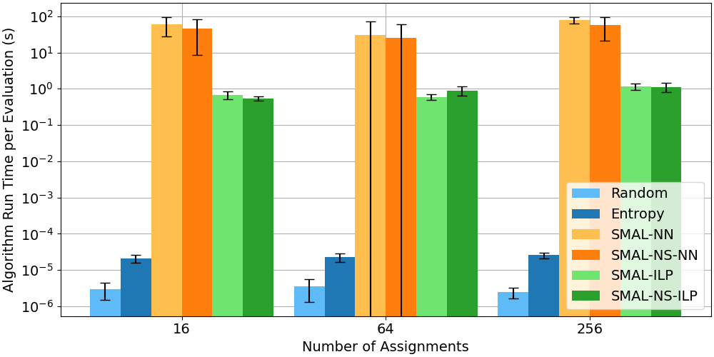
We show the actual algorithm run time as a function of the number of possible assignments (Figure 10). As expected, Random and Entropy are fastest, since they involve calling a pseudo-random number generator and simple formulas. SMAL-NN takes the longest time, and stochastic gradient descent dominates the run time. SMAL-NS-NN takes less time than SMAL-NN because the time for pretraining the NS network is not included and the average number of labeled examples is less. SMAL-ILP and SMAL-NS-ILP take around the same time, i.e., about 1 second. As might be expected from our analysis (Section 5.5.3, Equation 8), the ILP solver, Popper, dominates the run time. However, the run time does not increase much as the number of assignments increases from 16 to 256.

Interpretation.

SMAL-NN does not efficiently predict the next assignment to test, due to the overhead of stochastic gradient descent. On the other hand, the computational cost of SMAL-ILP and SMAL-NS-ILP is higher ( $\sim 1$ second) than that of Random and Entropy (microseconds, Figure 10). While we assume system tests (33 seconds each) dominate run time, this assumption will not hold for every use case. For instance, if application load changes dynamically at run-time at unpredictable intervals, short system tests with short algorithm run times may be preferred.

7 Conclusion and Future Work

We addressed the task-to-processor assignment problem by using expert domain knowledge and prior experience to guide the search. A tool for automatically configuring task-to-processor assignment is needed because an optimal task-to-processor assignment depends on hardware and application load, and the default Linux scheduler does not always perform as well as an optimal assignment. Furthermore, human-readable, logical task-to-processor assignment policies may enable interesting new possibilities, such as providing researchers a tool for deciding when and how two systems are different. While we use task-to-processor assignment as an example, we expect our approach generalizes to other auto-configuration problems when the appropriate background information is included.

Future work.

Our research opens several opportunities for further research:

$\blacksquare$

What is the limit on the number of tasks/processors our approach can handle?
$\blacksquare$

Can we generate policies invariant to the number of tasks?
$\blacksquare$

Can our approach be extended to systems with dynamic application load?
$\blacksquare$

Can we quantify interpretability of background information and policies?
$\blacksquare$

How easy is it for systems experts to generate background information for new tasks?

We begin answering the first two questions in Appendix C by providing list-based background relations. Finally, we plan to extend our approach to more difficult auto-configuration problems, such as configuring network parameters and process priorities.

References

[1] Liang Bao, Xin Liu, Ziheng Xu, and Baoyin Fang. AutoConfig: Automatic configuration tuning for distributed message systems. In ACM/IEEE International Conference on Automated Software Engineering, pages 29–40, 2018. doi:10.1145/3238147.3238175.
[2] Rudy Belliardi, Dorr Josef, Thomas Enzinger, Florian Essler, Janós Farkas, Hantel Mark, Maximilian Riegel, Marius-Petru Stanica, Guenter Steindl, Reiner Wamßer, Karl Weber, and Steven Zuponcic. Use cases IEC/IEEE 60802. Technical Report V1.3, IEEE, 2018.
[3] Bokhari. On the mapping problem. IEEE Transactions on Computers, 100(3):207–214, 1981. doi:10.1109/TC.1981.1675756.
[4] Christopher Bryant, Stephen Muggleton, Douglas Kell, Philip Reiser, Ross King, and Stephen Oliver. Combining inductive logic programming, active learning and robotics to discover the function of genes. Electronic Transactions in Artificial Intelligence, 5(B), 2001. URL: http://www.ep.liu.se/ej/etai/2001/001/.
[5] CFS scheduler. https://www.kernel.org/doc/Documentation/scheduler/sched-design-CFS.txt. Accessed: 2025-01-15.
[6] Jian Chen and Lizy John. Energy-aware application scheduling on a heterogeneous multi-core system. In IEEE International Symposium on Workload Characterization, pages 5–13, 2008.
[7] Andrew Cropper and Sebastijan Dumančić. Inductive logic programming at 30: A new introduction. Journal of Artificial Intelligence Research, 74:765–850, 2022. doi:10.1613/JAIR.1.13507.
[8] Andrew Cropper and Rolf Morel. Learning programs by learning from failures. Machine Learning, 110(4):801–856, 2021. doi:10.1007/S10994-020-05934-Z.
[9] Eduardo Cruz, Laércio Lima Pilla, and Philippe Navaux. An efficient algorithm for communication-based task mapping. In Euromicro International Conference on Parallel, Distributed, and Network-Based Processing. IEEE, 2015.
[10] Brahmaiah Gandham and Praveen Alapati. OCC pinning: Optimizing concurrent computations through thread pinning. In Workshop on Advanced Tools, Programming Languages, and PLatforms for Implementing and Evaluating algorithms for Distributed Systems, pages 1–5, 2024. doi:10.1145/3663338.3665829.
[11] Nathan Hanford, Vishal Ahuja, Matthew Farrens, Dipak Ghosal, Mehmet Balman, Eric Pouyoul, and Brian Tierney. Improving network performance on multicore systems: Impact of core affinities on high throughput flows. Future Generation Computer Systems, 56:277–283, 2016. doi:10.1016/J.FUTURE.2015.09.012.
[12] Nen-Fu Huang and Wen-Yen Tsai. qcAffin: A hardware topology aware interrupt affinitizing and balancing scheme for multi-core and multi-queue packet processing systems. IEEE Transactions on Parallel and Distributed Systems, 27(6), 2016. doi:10.1109/TPDS.2015.2453960.
[13] Ross King, Jem Rowland, Stephen Oliver, Michael Young, Wayne Aubrey, Emma Byrne, Maria Liakata, Magdalena Markham, Pinar Pir, Larisa Soldatova, Andrew Sparkes, Kenneth Whelan, and Amanda Clare. The automation of science. Science, 324(5923):85–89, 2009.
[14] Ross King, Kenneth Whelan, Ffion Jones, Philip Reiser, Christopher Bryant, Stephen Muggleton, Douglas Kell, and Stephen Oliver. Functional genomic hypothesis generation and experimentation by a robot scientist. Nature, 427(6971):247–252, 2004.
[15] Tobias Klug, Michael Ott, Josef Weidendorfer, and Carsten Trinitis. autopin — automated optimization of thread-to-core pinning on multicore systems. Transactions on High-Performance Embedded Architectures and Compilers, pages 219–235, 2011. doi:10.1007/978-3-642-19448-1_12.
[16] Zexin Li, Yuqun Zhang, Ao Ding, Husheng Zhou, and Cong Liu. Efficient algorithms for task mapping on heterogeneous CPU/GPU platforms for fast completion time. Journal of Systems Architecture, 114, 2021. doi:10.1016/J.SYSARC.2020.101936.
[17] Sorin Manolache, Petru Eles, and Zebo Peng. Task mapping and priority assignment for soft real-time applications under deadline miss ratio constraints. ACM Transactions on Embedded Computing Systems, 7(2):1–35, 2008. doi:10.1145/1331331.1331343.
[18] Miloš Panić, Sebastian Kehr, Eduardo Quiñones, Bert Boddecker, Jaume Abella, and Francisco Cazorla. RunPar: An allocation algorithm for automotive applications exploiting runnable parallelism in multicores. In International Conference on Hardware/Software Codesign and System Synthesis, pages 1–10. Association for Computing Machinery, 2014.
[19] Don Pannell. Choosing the right TSN tools to meet a bounded latency. Technical report, NXP, 2021.
[20] Stuart Russell and Peter Norvig. Artificial Intelligence: A Modern Approach. Pearson, 3 edition, 2009.
[21] James Salehi, James Kurose, and Don Towsley. The effectiveness of affinity-based scheduling in multiprocessor network protocol processing (extended version). IEEE/ACM Transactions on Networking, 4(4):516–530, 1996. doi:10.1109/90.532862.
[22] Xi Tao, Weipeng Cao, Yinghui Pan, Ye Liu, and Zhong Ming. Improving QoS of workloads with CPU pinning: A deep reinforcement learning approach. In IEEE/ACM International Symposium on Quality of Service, pages 1–2, 2024. doi:10.1109/IWQOS61813.2024.10682839.
[23] Alaa Tharwat and Wolfram Schenck. A survey on active learning: State-of-the-art, practical challenges and research directions. Mathematics, 11(4):820, 2023.

Appendix A Expressing Domain Knowledge as a Logic Program

To express domain knowledge as a logic program, we provide the relations required to describe sets of assignments which satisfy the real-time requirement. If this is achieved, the solver will likely generate policies that cover satisfactory assignments for a specific scenario. We use a few techniques to obtain such relations:

From experimentation.

By running small-scale experiments and visualizing the solution space. For example, after seeing Figure 3(a), we noticed that the best (and worst) solutions have tasks on the network-interrupted processor. Also, the best solutions have tasks sharing a processor (and prior work in load balancing suggests that sometimes tasks should not share a processor [12, 10]). We described these relationships with the relations on_intr_lp, shares_lp, and diff_lps. We then run the ILP solver and check that the policy describes the solution space.

From domain knowledge.

By direct description of domain knowledge. For example, before running experiments with CPUs equipped with hyper-threading, we knew that two LPs on the same core are likely to influence one another, e.g., through context switching triggered by network interrupts. Thus, we added predicates on_intr_ht and off_intr_ht to capture this intuition.

From procedure.

By enabling predicate invention to procedurally generate predicates. For example, in Section 5.1, predicate invention results in a symbol for the “parent” relationship, which simplifies the hypothesis for “grandparent”. In some of our experiments, we tested enabling predicate invention, but the results were the same as without predicate invention.

Appendix B Influence of Nearest Scenario Data on SMAL-NS-ILP

To get an idea of how data from the nearest scenario influences SMAL-NS-ILP (and SMAL-NS-NN), we compare the “% Positives” to the “% NS Positives Overlap” in Table 4. Let $p$ be the ratio of “Positives” and $q$ be the ratio of “NS Positives Overlap”. If selecting assignments uniformly at random from the test scenario, the probability of the first assignment being positive is $p$ (and $\geq p$ in subsequent selections). If selecting assignments which are positive according to the nearest scenario uniformly at random, the probability of the first successful assignment is $q$ (and $\geq q$ in subsequent selections). Since SMAL-NS-ILP selects from the NS positives first, we expect SMAL-NS-ILP to do better than SMAL-ILP when $p<q$ (and worse when $p>q$ ). For example, if every NS positive is also positive in the test scenario, $q=1$ , and the first selection is guaranteed to be positive. Likewise, if every NS positive is negative in the test scenario, $q=0$ , and at least every NS positive will be tested before a positive assignment is found.

However, there are two other factors, besides the nearest scenario’s data, influencing the performance of SMAL-NS-ILP. First, the NS policy $\bar{\pi}$ may not perfectly fit the NS data, so NS positives are not necessarily the same as positives according to $\bar{\pi}$ . Second, the search order of SMAL-NS-ILP is influenced by $\bar{\pi}$ , so the intermediate policy is trained on a different distribution of examples than SMAL-ILP. Nonetheless, a large “% NS Positives Overlap” is a prerequisite for SMAL-NS-ILP (and SMAL-NS-NN) to work as intended.

Appendix C Scaling Up the Number of Tasks

We see in Section 5.5.3 that optimal ILP solvers may not scale well with the number of variables; however, practical problems demand assignment of possibly hundreds of tasks. Indeed, we find Popper [8], with our proposed background (Section 5.2), does not run with 12 or more tasks. A possible solution is to develop ILP solvers which return approximate, but high quality, solutions. We explore another possible solution: represent $m$ tasks with a constant number of variables. This is achieved by providing background relations between lists of tasks.

C.1 List-Based Domain Knowledge

We express assignments as a set of relations between two lists: a list of critical tasks and a list of background tasks. The new background information is shown in Listing 5. An example policy, trained on the data in Figure 5, is shown in Listing 6. The learned policy is read as “No background tasks are on the interrupted LP and the smallest number of background tasks sharing an LP with a critical task is 1.”

Listing 5: Background information for SMAL-ILP and SMAL-NS-ILP in the 12-task experiments.

⬇

% A number of items.

zero(0). one(1). two(2). three(3). four(4). five(5). six(6).

% Which logical processor (LP) is interrupted by the network.

on_intr_lp(0).

% Which LPs are not interrupted by the network.

off_intr_lp(1). off_intr_lp(2). off_intr_lp(3).

% The number of tasks on the same LP interrupted by the network.

on_intr_lp_count([], 0).

on_intr_lp_count([Head|Tail], N):-

on_intr_lp(Head), on_intr_lp_count(Tail, M), N is M + 1.

on_intr_lp_count([Head|Tail], N):-

off_intr_lp(Head), on_intr_lp_count(Tail, N).

% Max number of tasks in List2 sharing an LP with a task in List1.

max_shared([], _, 0).

max_shared([Head|Tail], List2, N):-

max_shared(Tail, List2, K),

findall(X, (X = Head, member(X, List2)), Matches),

length(Matches, M), N is max(M, K).

% Min number of tasks in List2 sharing an LP with a task in List1.

min_shared([], _, 0).

min_shared([Head], List2, N):-

findall(X, (X = Head, member(X, List2)), Matches),

length(Matches, N).

min_shared([Head,Head2|Tail], List2, N):-

min_shared([Head2|Tail], List2, K),

findall(X, (X = Head, member(X, List2)), Matches),

length(Matches, M), N is min(M, K).

Listing 6: Hypothesis generated from Dataset 1, Scenario S2 (Figure 5).

⬇

assign(V0,V1):-

on_intr_lp_count(V1,V2), zero(V2),

min_shared(V0,V1,V3), one(V3).

Besides reducing the problem from $m$ variables to 2 variables, list-based hypotheses are agnostic to the number of tasks. This makes it technically possible to apply policies learned with one number of (or various numbers of) tasks and apply the policy (using SMAL-NS-ILP) to a scenario with a different number of tasks.

C.2 Experiments

Setup.

We test the Raspberry Pi 4B setup, this time with 6 background and 6 critical tasks, running on Host 2 (Figure 1). The number of possible assignments is $4^{12}=16777216$ . Because the assignment space is large, the optimal 99.9th percentile latency is unknown. Thus, we choose the deadline to be within 10% of the best latency found after 100 random system tests. Also, assignments are tested live rather than on a prerecorded dataset.

For SMAL-ILP and SMAL-NS-ILP, we sample 100 assignments uniformly at random, from the assignment space, for examples. We choose Dataset 1, Scenario S4 for the nearest scenario for SMAL-NS-ILP, where $m=4$ , while the test scenario has $m=12$ .

Results.

The result is in Table 5. Entropy again performs poorly, even with 12 tasks. SMAL-ILP performs better than Random; although, the variance is high in both cases. SMAL-NS-ILP does not do as well this time. This is because a policy for labeling positive assignments for the 4-task scenario does not generalize to the 12-task scenario.

Table 5: Host 2 with 6 background and 6 critical tasks. The deadline was set to

789\text{\,}\mathrm{\SIUnitSymbolMicro s}

. Showing average

\pm

sample standard deviation over 30 trials. Run time per iteration excludes the time to evaluate the system (i.e., excludes

33\text{\,}\mathrm{s}

). A trial was terminated after 100 evaluations if no assignment meeting the deadline was found (i.e., the worst possible result is 100 evaluations.)

	Random	Entropy	SMAL-ILP	SMAL-NS-ILP
Number of Evaluations	$35.4\pm 29.6$	$94.8\pm 17.7$	$22.7\pm 21.1$	$38.2\pm 23.7$
Run Time per Iteration (s)	$0.00\pm 0.00$	$1.77\pm 0.07$	$10.3\pm 0.18$	$10.4\pm 0.21$

[bib.bib1] [1] Liang Bao, Xin Liu, Ziheng Xu, and Baoyin Fang. AutoConfig: Automatic configuration tuning for distributed message systems. In ACM/IEEE International Conference on Automated Software Engineering, pages 29–40, 2018. doi:10.1145/3238147.3238175.

[bib.bib2] [2] Rudy Belliardi, Dorr Josef, Thomas Enzinger, Florian Essler, Janós Farkas, Hantel Mark, Maximilian Riegel, Marius-Petru Stanica, Guenter Steindl, Reiner Wamßer, Karl Weber, and Steven Zuponcic. Use cases IEC/IEEE 60802. Technical Report V1.3, IEEE, 2018.

[bib.bib3] [3] Bokhari. On the mapping problem. IEEE Transactions on Computers, 100(3):207–214, 1981. doi:10.1109/TC.1981.1675756.

[bib.bib4] [4] Christopher Bryant, Stephen Muggleton, Douglas Kell, Philip Reiser, Ross King, and Stephen Oliver. Combining inductive logic programming, active learning and robotics to discover the function of genes. Electronic Transactions in Artificial Intelligence, 5(B), 2001. URL: http://www.ep.liu.se/ej/etai/2001/001/.

[bib.bib5] [5] CFS scheduler. https://www.kernel.org/doc/Documentation/scheduler/sched-design-CFS.txt. Accessed: 2025-01-15.

[bib.bib6] [6] Jian Chen and Lizy John. Energy-aware application scheduling on a heterogeneous multi-core system. In IEEE International Symposium on Workload Characterization, pages 5–13, 2008.

[bib.bib7] [7] Andrew Cropper and Sebastijan Dumančić. Inductive logic programming at 30: A new introduction. Journal of Artificial Intelligence Research, 74:765–850, 2022. doi:10.1613/JAIR.1.13507.

[bib.bib8] [8] Andrew Cropper and Rolf Morel. Learning programs by learning from failures. Machine Learning, 110(4):801–856, 2021. doi:10.1007/S10994-020-05934-Z.

[bib.bib9] [9] Eduardo Cruz, Laércio Lima Pilla, and Philippe Navaux. An efficient algorithm for communication-based task mapping. In Euromicro International Conference on Parallel, Distributed, and Network-Based Processing. IEEE, 2015.

[bib.bib10] [10] Brahmaiah Gandham and Praveen Alapati. OCC pinning: Optimizing concurrent computations through thread pinning. In Workshop on Advanced Tools, Programming Languages, and PLatforms for Implementing and Evaluating algorithms for Distributed Systems, pages 1–5, 2024. doi:10.1145/3663338.3665829.

[bib.bib11] [11] Nathan Hanford, Vishal Ahuja, Matthew Farrens, Dipak Ghosal, Mehmet Balman, Eric Pouyoul, and Brian Tierney. Improving network performance on multicore systems: Impact of core affinities on high throughput flows. Future Generation Computer Systems, 56:277–283, 2016. doi:10.1016/J.FUTURE.2015.09.012.

[bib.bib12] [12] Nen-Fu Huang and Wen-Yen Tsai. qcAffin: A hardware topology aware interrupt affinitizing and balancing scheme for multi-core and multi-queue packet processing systems. IEEE Transactions on Parallel and Distributed Systems, 27(6), 2016. doi:10.1109/TPDS.2015.2453960.

[bib.bib13] [13] Ross King, Jem Rowland, Stephen Oliver, Michael Young, Wayne Aubrey, Emma Byrne, Maria Liakata, Magdalena Markham, Pinar Pir, Larisa Soldatova, Andrew Sparkes, Kenneth Whelan, and Amanda Clare. The automation of science. Science, 324(5923):85–89, 2009.

[bib.bib14] [14] Ross King, Kenneth Whelan, Ffion Jones, Philip Reiser, Christopher Bryant, Stephen Muggleton, Douglas Kell, and Stephen Oliver. Functional genomic hypothesis generation and experimentation by a robot scientist. Nature, 427(6971):247–252, 2004.

[bib.bib15] [15] Tobias Klug, Michael Ott, Josef Weidendorfer, and Carsten Trinitis. autopin — automated optimization of thread-to-core pinning on multicore systems. Transactions on High-Performance Embedded Architectures and Compilers, pages 219–235, 2011. doi:10.1007/978-3-642-19448-1_12.

[bib.bib16] [16] Zexin Li, Yuqun Zhang, Ao Ding, Husheng Zhou, and Cong Liu. Efficient algorithms for task mapping on heterogeneous CPU/GPU platforms for fast completion time. Journal of Systems Architecture, 114, 2021. doi:10.1016/J.SYSARC.2020.101936.

[bib.bib17] [17] Sorin Manolache, Petru Eles, and Zebo Peng. Task mapping and priority assignment for soft real-time applications under deadline miss ratio constraints. ACM Transactions on Embedded Computing Systems, 7(2):1–35, 2008. doi:10.1145/1331331.1331343.

[bib.bib18] [18] Miloš Panić, Sebastian Kehr, Eduardo Quiñones, Bert Boddecker, Jaume Abella, and Francisco Cazorla. RunPar: An allocation algorithm for automotive applications exploiting runnable parallelism in multicores. In International Conference on Hardware/Software Codesign and System Synthesis, pages 1–10. Association for Computing Machinery, 2014.

[bib.bib19] [19] Don Pannell. Choosing the right TSN tools to meet a bounded latency. Technical report, NXP, 2021.

[bib.bib20] [20] Stuart Russell and Peter Norvig. Artificial Intelligence: A Modern Approach. Pearson, 3 edition, 2009.

[bib.bib21] [21] James Salehi, James Kurose, and Don Towsley. The effectiveness of affinity-based scheduling in multiprocessor network protocol processing (extended version). IEEE/ACM Transactions on Networking, 4(4):516–530, 1996. doi:10.1109/90.532862.

[bib.bib22] [22] Xi Tao, Weipeng Cao, Yinghui Pan, Ye Liu, and Zhong Ming. Improving QoS of workloads with CPU pinning: A deep reinforcement learning approach. In IEEE/ACM International Symposium on Quality of Service, pages 1–2, 2024. doi:10.1109/IWQOS61813.2024.10682839.

[bib.bib23] [23] Alaa Tharwat and Wolfram Schenck. A survey on active learning: State-of-the-art, practical challenges and research directions. Mathematics, 11(4):820, 2023.