Analysis of EDF for Real-Time Multiprocessor Systems with Resource Sharing

Agrawal, Kunal; Baruah, Sanjoy; Fineman, Jeremy T.; Marchetti-Spaccamela, Alberto; Zhao, Jinhao

doi:10.4230/LIPIcs.ECRTS.2025.15

Analysis of EDF for Real-Time Multiprocessor Systems with Resource Sharing

Kunal Agrawal

Washington University in St. Louis, MO, USA Sanjoy Baruah

Washington University in St. Louis, MO, USA Jeremy T. Fineman

Georgetown University, Washington, D.C., USA Alberto Marchetti-Spaccamela

University of Rome, Italy Jinhao Zhao

Washington University in St. Louis, MO, USA

Abstract

The classic Earliest Deadline First (EDF) algorithm is widely studied and used due to its simplicity and strong theoretical performance, but has not been rigorously analyzed for systems where jobs may execute critical sections protected by shared locks. Analyzing such systems is often challenging due to unpredictable delays caused by contention. In this paper, we propose a straightforward generalization of EDF, called EDF-Block. In this generalization, the critical sections are executed non-preemptively, but scheduling and lock acquisition priorities are based on EDF. We establish lower bounds on the speed augmentation required for any non-clairvoyant scheduler (EDF-Block is an example of non-clairvoyant schedulers) and for EDF-Block, showing that EDF-Block requires at least 4.11× speed augmentation for jobs and 4× for tasks. We then provide an upper bound analysis, demonstrating that EDF-Block requires speedup of at most 6 to schedule all feasible job and task sets.

Keywords and phrases:

Real-Time Scheduling, Non-Clairvoyant Scheduling, EDF, Competitive Analysis, Shared Resources

Funding:

Kunal Agrawal: NSF CCF-2106699, CCF-2107280, PPoSS-2216971.

Sanjoy Baruah: NSF CNS-2141256, CPS-2229290.

Jeremy T. Fineman: NSF CCF-2106759, CCF-1918989.

Copyright and License:

2012 ACM Subject Classification:

Theory of computation

\rightarrow

Online algorithms ; Mathematics of computing

\rightarrow

Mathematical optimization ; Computer systems organization

\rightarrow

Real-time operating systems

DOI:

10.4230/LIPIcs.ECRTS.2025.15

Event:

37th Euromicro Conference on Real-Time Systems (ECRTS 2025)

Editors:

Renato Mancuso

Series and Publisher:

Leibniz International Proceedings in Informatics, Schloss Dagstuhl – Leibniz-Zentrum für Informatik

1 Introduction

In this paper, we consider a basic problem of scheduling real-time jobs on a multiprocessor platform where jobs may need access to a shared resource. We ask the question: what is the performance of the simplest possible generalization of the basic earliest deadline first algorithm for this problem?

The Earliest Deadline First (EDF) algorithm is a simple, intuitive, and widely studied scheduling strategy for jobs with deadline constraints. Jobs are ordered by their deadlines so that the earliest deadline job has the highest priority. Given $m$ uniform speed processors, at any time instant, we run the $m$ highest priority jobs preemptively. It is known that this strategy, also called global EDF in the multiprocessor setting, has good theoretical performance. For instance, for jobs with deadlines, a classic result [29] shows that EDF provides a speedup bound of 2 indicating that if a set of jobs or tasks is feasible on processors of speed 1, and EDF can schedule them on processors of speed 2.

Extending EDF schedulability analysis to incorporate shared resources introduces additional challenges. When we have shared resources that require exclusive access, a scheduler must answer two questions: (1) If more than $m$ jobs are active, which jobs should execute on the $m$ available processors? EDF says the $m$ jobs with the earliest deadlines. (2) If multiple jobs are waiting on a lock to execute a critical section, then which job should get the lock? By the logic of EDF, the job with the earliest deadline should get the lock. This simple algorithm has several advantages: It is non-clairvoyant – it needn’t know when jobs will arrive or any characteristics of the jobs (execution time, duration of the critical section, etc.) except their deadlines. This simple generalization of EDF has not been analyzed in the prior literature. In this paper, we ask the question: What is the performance of EDF (in terms of speedup bounds) for the simplest model of jobs and tasks with shared resources protected by locks? In particular, we limit ourselves to sequential tasks, a single lock and each job has at most one critical section protected by this lock. We consider both online job scheduling where jobs are released over time as well as sporadic task scheduling for recurrent tasks. Our contributions in this paper are as follows:

$\blacksquare$

We define EDF-Block as a simple generalization of EDF for scheduling sequential jobs on uniform multiprocessors with $m$ processors.
$\blacksquare$

We establish a lower bound on any non-clairvoyant scheduler for jobs. In particular, we show that any scheduler that does not know the execution characteristics of jobs when they arrive requires speedup of at least 4 in order to schedule all feasible job sets.
$\blacksquare$

We also establish lower bounds for EDF-Block. In particular, EDF-Block requires speedup at least $\approx 4.11$ (for large $m$ ) for jobs. For constrained deadline sporadic tasks, EDF-Block requires speed at least $4$ (for large $m$ ).
$\blacksquare$

We establish an upper bound of $6$ for speedup for EDF-Block for both jobs and tasks. Therefore, the actual speedup bound for EDF-Block is between $4.11$ and $6$ for jobs and between $4$ and $6$ for tasks. This upper bound is based on simple feasibility conditions only; therefore, it can be used as a schedulability test.

The remainder of this paper is structured as follows: Section 2 provides a formal definition of the problem. Section 3 introduces our scheduling algorithm. Section 4 discusses theoretical lower bounds on the performance of EDF-Block and other non-clairvoyant schedulers. Section 5 presents an upper bound analysis for EDF-Block for jobs which automatically generalizes to tasks. Section 6 runs a simulation, comparing EDF-Block and an existing algorithm on randomly generated tasks. Sections 7 and 8 present related work and conclusions.

2 Problem Definition and Preliminaries

In this section, we start by formally defining the problem for jobs, provide other relevant definitions and finally generalize the problem to sporadic tasks.

Problem Definition For Jobs

We consider the following problem:

Definition 1 (Job Scheduling with Locks: $(m,\{J_{i}\})$ ).

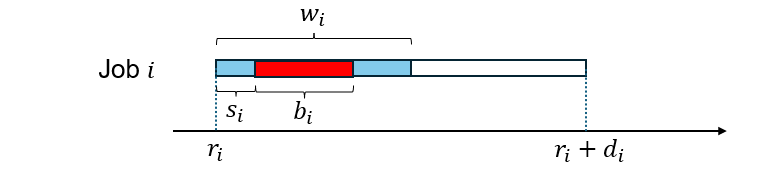
We consider a system $\mathcal{J}$ of $n$ jobs that must be scheduled on $m$ processors or cores. Each job can acquire a lock (in order to execute a critical section) once during its execution. Thus, each job $J_{i}$ is characterized by the tuple $(r_{i},d_{i},w_{i},b_{i},s_{i})$ where:

$\blacksquare$

$r_{i}$ is the release time when the job becomes available to schedule;
$\blacksquare$

$d_{i}$ is the relative deadline – the job must complete by time $r_{i}+d_{i}$ ;
$\blacksquare$

$w_{i}$ is the work or the execution requirement of the job;
$\blacksquare$

$b_{i}$ is the duration of the critical section; and
$\blacksquare$

$s_{i}$ is the execution duration of the job before entering the critical section.

A job may be preempted outside its critical section. However, only one job can hold a lock (execute the critical section) at a time. In addition, once a job acquires the lock, it does not release the lock and cannot be preempted until the end of its critical section – that is, after it has executed for $b_{i}$ additional time.

Refer to caption — Figure 1: Example for a job as $(r_{i},d_{i},w_{i},b_{i},s_{i})$ .

In addition to this basic problem, we make a further assumption that no critical section is “too long”. In particular, if two jobs, say $J_{a}$ and $J_{b}$ overlap in their intervals (each job’s release time is before the other job’s deadline) and say $J_{a}$ ’s critical section is longer than the duration of $J_{b}$ ’s scheduling window (the interval from its release time to deadline), then, $J_{a}$ may hold the lock for $J_{b}$ ’s entire life cycle disallowing $J_{b}$ from ever acquiring the lock and executing. Specially, for non-clairvoyant schedulers, such systems can be very difficult to schedule. Therefore, we make the following assumption on our systems:

Definition 2 (Limited Blocking).

If two jobs’ intervals overlap, i.e., $r_{j}+d_{j}>r_{i}$ and $r_{i}+d_{i}>r_{j}$ , then $b_{j}\leq d_{i}$ and $b_{i}\leq d_{j}$ .

Valid Schedule

We now define a valid schedule $S$ for a system of such jobs. This is a generalization of the normal definition of a multiprocessor schedule apart from the last constraint which relates to critical sections.

Definition 3 (Valid Schedule for Jobs).

Given a problem $(m,\{J_{i}\})$ from Definition 1, the schedule $S=\{K_{i}\}_{i=1}^{n}$ comprises $n$ sets of intervals, with $K_{i}$ denoting the intervals when the $i$ ’th job is executing. Schedule $S$ is valid if and only if each $K_{i}$ matches all the following:

$\blacksquare$

Each interval in $K_{i}$ is $\subseteq[r_{i},r_{i}+d_{i}]$
$\blacksquare$

$\lambda(K_{i})=w_{i}$ , where $\lambda$ is the Lebesgue measure of (the sum of interval lengths in) the set.
$\blacksquare$

For each time step $j$ , $\sum_{i}\mathbb{I}(j\in K_{i})\leq m$ – i.e., at most $m$ jobs are executing at each time-step
$\blacksquare$

Only one job is executing the critical section at a time, as in Definition 1.
$\blacksquare$

The critical section of each job is continuous, as in Definition 1.

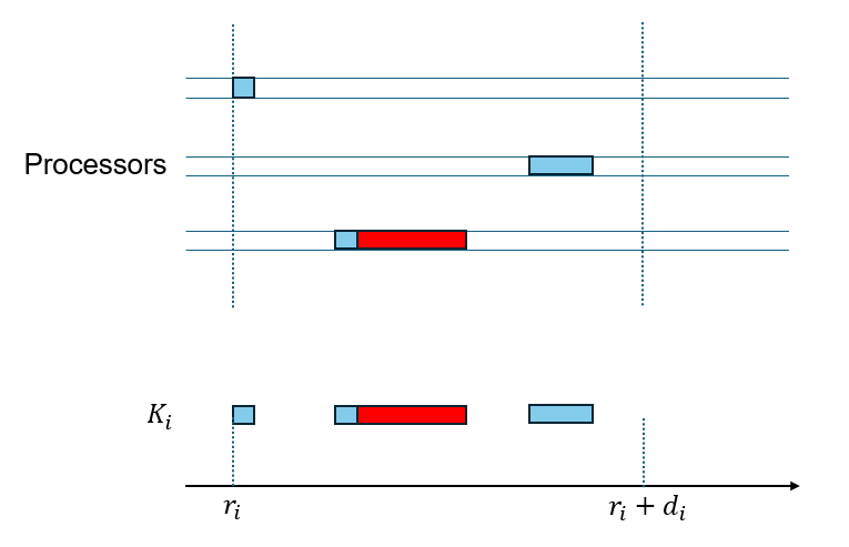
(We point out that constructing an actual particular schedule requires more information than is provided in Definition 3 – such as which processor is used to execute each part of the job. Figure 2 shows two schedules for a single job which both have the same $K_{i}$ ’s. However, since jobs outside the critical section are preemptive and can run on any processor, a valid schedule can be reconstructed given all $K_{i}$ ’s. Therefore, Definition 3 is sufficient for checking for correctness of a schedule.)

Sporadic Tasks

We also investigate this problem in sporadic tasks, defined as follows.

Definition 4 (Task with Locks).

A task $T=(w_{i},b_{i},d_{i},t_{i})$ generates a sequence of jobs with relative deadline $d_{i}$ , work $w_{i}$ and blocking duration $b_{i}$ . The jobs arrive with a minimum inter-arrival time of at least $t_{i}$ .

Note that this definition does not define $s_{i}$ which is the starting time of the critical section within a job. For the purposes of this definition, we assume that $s_{i}$ can be arbitrary as long as it is between $0$ and $(w_{i}-b_{i})$ and it can be different for different jobs of the task. (Note that this only makes the scheduling problem harder since the scheduler has less information. For the purposes of scheduler and schedulability test, the algorithm must be able to handle all possible values for $s_{i}$ for each individual job.) The reason for this assumption is pragmatic. Generally for real-time task scheduling, execution durations $w_{i}$ ’s (and presumably $b_{i}$ ) are estimated using some worst-case analysis methods and are upper bounds. Most reasonable schedulers should work even if the actual execution duration is shorter. However, if we are to use $s_{i}$ to do schedulability analysis, an upper bound is unlikely to be useful – we would need its exact value. However, in real systems, the start of the critical section for each job of a task may be different due to various factors related to the program and the system itself. Therefore, estimating $s_{i}$ is likely to be both difficult (if not impossible) and not very useful. We therefore assume that the task system doesn’t know it.

Given this definition of tasks, a task system with locks consists of $n$ tasks which must be executed on a platform with $m$ processors. We also must have a limited blocking condition as follows since a job of any task may overlap with a job of any other task:

Definition 5 (Limited Blocking for Sporadic Tasks).

For all tasks $i, j$ , $b_{i}\leq d_{j}$ .

Speedup Bounds

In this paper, we analyze an online algorithm for scheduling jobs with critical sections and deadlines. Given a system of jobs or tasks, we will characterize the performance of a scheduler using a version of competitive analysis. In particular, we ask the question: given a feasible input on $m$ processors of speed 1, how much speed does the online algorithm require in order to guarantee schedulability in the worst case?

There are two ways equivalent of thinking about speedup. One is to imagine that the machine itself has a larger speed, say $\sigma$ . The other is to reduce all the execution parameters $w, b, s$ by a factor of $\sigma$ . We will formally define the second version; however, one or the other is more convenient in different proofs and we will use the more convenient one as needed.

Definition 6 (Speed augmentation).

Consider a set of jobs $\mathcal{J}=\{J_{i}\}$ ; we define a $\sigma$ -augmented set $\mathcal{J^{\prime}}$ consisting of $J_{i}^{\prime}=(r_{i},d_{i},w_{i}/\sigma,b_{i}/\sigma,s_{i}/\sigma)$ . We say that an algorithm $A$ ’s speedup bound is $\sigma$ if $A$ can correctly schedule $\sigma$ -augmented jobs $\mathcal{J^{\prime}}$ for all feasible systems of jobs $(m,\mathcal{J^{\prime}})$ on $m$ processors.

The definition of tasks is analogous. An algorithm $A$ ’s speedup bound is $\sigma$ if it can schedule all (augmented) jobs systems that all feasible task systems can generate.

Non-clairvoyant Schedulers

Schedulers for tasks and jobs can be clairvoyant or non-clairvoyant. In this paper, we analyze EDF-Block, which is a non-clairvoyant scheduler. There are many ways of defining clairvoyance, non-clairvoyance and semi-clairvoyance. In this paper, we use a strong definition where the scheduler has very little information in advance.

Definition 7 (non-clairvoyant scheduler).

A non-clairvoyant scheduler is a scheduler that doesn’t know the arrival times of jobs before they arrive. In addition, it doesn’t know any characteristics of jobs such as their work $w_{i}$ , critical section length $b_{i}$ , or start of blocking time $s_{i}$ . It only knows its deadline when the job arrives.

Nonclairvoyance for tasks is often harder to define since for most task systems, one assumes that some estimate of the execution requirement of tasks is known in advance. For the purposes of this paper, however, we define nonclairvoyance for tasks as a system that generates a non-clairvoyant system of jobs.

3 EDF-Block: EDF for Jobs with Critical Sections

In this paper, we will analyze a relatively straightforward algorithm for jobs with deadlines and critical sections. We call this algorithm EDF-Block, and it is a simple generalization of the earliest deadline first (EDF) algorithm. Each job has a priority based on its deadline – the earliest deadline job has the highest priority and executes according to this priority. EDF-Block works as follows:

$\blacksquare$

Run EDF on the jobs preemptively. If no job is waiting for a lock, the $m$ jobs with the earliest deadline execute on the $m$ processors; if some job is holding the lock, that job and the $(m-1)$ jobs with earliest deadline that do not require the lock execute.
$\blacksquare$

When a job wants the lock, if no one is holding it, then the job gets it. Otherwise, it blocks and waits for the lock. When multiple jobs are waiting on a lock, the job with the earliest deadline acquires the lock. Once a job acquires a lock, it runs non-preemptively until its critical section finishes.

For intuition, let us consider (and compare) two situations where EDF-Block experiences inversions where a job with an earlier deadline waits on a job with a later deadline.

$\blacksquare$

This first circumstance is somewhat intuitive: A higher priority job may wait on a lower priority job since it wants a lock that the lower priority job is holding. If a lower priority job, say $J_{b}$ , is holding a lock and a higher priority job, say $J_{a}$ reaches the beginning of its critical section, it has to yield its processor and wait for $J_{b}$ to complete. In the meanwhile, an even lower priority job, say $J_{c}$ can execute on the processor which $J_{a}$ was using. However, once $J_{b}$ finishes, either $J_{a}$ or someone of higher priority than $J_{a}$ will take the lock. Therefore, this type of inversion can happen only once per critical section and therefore, once per job since our jobs have only one critical section each.
$\blacksquare$

The second circumstance is more counter-intuitive and even jobs which do not require locks may wait on lower priority jobs to be released. Let us suppose that $m-1$ jobs are executing normally and the (current) $m$ ’th priority job, say $J_{b}$ is holding a lock. Now let us say a job, say $J_{a}$ is released. $J_{a}$ has a deadline after the earliest $m-1$ deadlines but before $J_{b}$ . $J_{a}$ is now the $m$ ’th priority job and should be able to execute. However, since $J_{b}$ is holding the lock, it must execute the critical section non-preemptively, and $J_{a}$ has to wait for $J_{b}$ to complete its critical section. Note that here, $J_{a}$ did not even want a lock and it was still blocked due to a lower priority job.

Note that EDF-Block, like EDF, is an online non-clairvoyant algorithm that does not need to know the future releases of jobs before they arrive. In addition, when the job arrives, the algorithm need not know the work $w_{i}$ , blocking time $b_{i}$ or start of block $s_{i}$ of jobs in advance, it need only know the job’s deadline.

4 Lower Bounds

In this section, we provide some lower bounds that characterize the performance of EDF-Block. We first show that any non-clairvoyant scheduler requires a speedup of at least 4 in order to schedule all feasible job systems. We then show specific lower bounds of EDF-Block.

In particular, we will compare online schedulers to a hypothetical optimal offline (clairvoyant) scheduler (called OPT) which knows everything about the jobs in advance and can construct the best possible schedule. In order to prove the lower bound of $\sigma$ , we will show that there exist systems of jobs (or tasks) where this offline scheduler can schedule these systems on $m$ processors of speed 1 while the online scheduler under consideration requires $m$ processors of at least $\sigma$ .

4.1 Lower bound for non-clairvoyant schedulers

We now prove a quite general theorem that shows that there exist job sets that can make any deterministic nonclairvoyant scheduler behave “badly.” As defined in Section 2, A non-clairvoyant scheduler is a scheduler that doesn’t know the arrival times of jobs before they arrive. In this proof, given a scheduler, we will construct a set of jobs that are “difficult” for that scheduler. Therefore, the particular job set depends on the behavior of the scheduling algorithm itself.

Theorem 1.

Any deterministic non-clairvoyant scheduler requires speed augmentation of at least $4-2/m$ to correctly schedule all feasible job systems where $m$ is the number of processors.

Proof.

We will construct a feasible job set to ensure that any given scheduler behaves badly. As mentioned above, some parameters of the example are scheduler dependent – in other words, the adversary knows the scheduling algorithm and designs the set of jobs which are bad for this scheduler from the perspective of speedup.

The overall job set $J$ includes a subset $J^{*}$ of (approximately) $m^{2}$ jobs and one additional job $J_{0}$ . We will define $J^{*}$ with a parameter $P$ which we will define later – the value of $P$ depends on the actions of the non-clairvoyant scheduler.

1.

One job of $J^{*}$ , say job $x$ , has both work and critical section length $P-m^{2}\epsilon$ ( $\epsilon$ is very small) – intuitively, this is a long job with a long critical section.
2.

Another job of $J^{*}$ , say job $y$ , has critical section length $\epsilon$ at the very beginning ( $s_{y}=0$ ) and has work of $P$ – this is a long job with a short critical section at the beginning.
3.

All other jobs of $J^{*}$ have critical section length $\epsilon$ time at the beginning and have work of $(m-2)(P-m^{2}\epsilon)/(m^{2}-2)$ – These are relatively short jobs with very small critical sections.¹¹1The parameters here are somewhat strange when $m=2$ . In this case, there are only jobs $x$ and $y$ in $J^{*}$ , and the resource augmentation ends up as $4-2/m=3$ .

At time $0$ , we release an outlying job $J_{0}$ (this is not in set $J^{*}$ ) with deadline $D$ which immediately demands the lock. Consider a non-clairvoyant scheduler (say with speed $\sigma$ ) which does not know anything about this job except its deadline. At some point, this scheduler starts executing this job and the job acquires the lock, say at time $t$ . The adversary has set $P=(D-t)/2$ . At this time $t$ , the set $J^{*}$ is released with relative deadline of all these newly released jobs as $P$ , and the job $J_{0}$ has both work and critical section $P$ .

First, we show that this set of jobs is feasible. The total work of $J^{*}$ is (roughly) $m P$ and the total blocking is $P$ . Starting from time $t$ , OPT will run the critical sections of all $m^{2}-1$ of $J^{*}$ jobs except job $x$ , then run $x$ and the portions outside the critical section. This takes $P$ time steps in total, so all jobs of $J^{*}$ finish at time $t+P$ . Then, $J_{0}$ runs for another $P$ steps and finishes at $D$ .

Now we show that any non-clairvoyant scheduler needs speed of at least $4$ to schedule all jobs correctly. Consider speed $\sigma$ which is sufficient for schedulability with this non-clairvoyant (NC) scheduler. Therefore, all the job’s execution parameters are divided by $\sigma$ . In this scheduler, job $J_{0}$ will complete at time $t+P/\sigma$ . At this time, the non-clairvoyant scheduler gives the lock to some arbitrary job from set $J^{*}$ since it cannot distinguish between them. This will happen to be the long blocking job $x$ and it will block out all the other jobs for time $(P-m^{2}\epsilon)/\sigma$ . Now say we don’t even worry about the blocking, but whichever jobs the NC scheduler executes all happen to be short jobs (none of them are the job $y$ ). These short jobs have total work $(m-2)(P-m^{2}\epsilon)$ , so they take another $(m-2)(P-m^{2}\epsilon)/(m\sigma)$ time to complete. And now we get to execute the job $y$ and it takes another $P/\sigma$ time. The time to complete $y$ should be no later than its deadline, which means:

t+\underbrace{P/\sigma}_{J_{0}}+\underbrace{(P-m^{2}\epsilon)/\sigma}_{x}+% \underbrace{(m-2)(P-m^{2}\epsilon)/m\sigma}_{others\ in\ J^{*}}+\underbrace{P/% \sigma}_{y}\leq t+P.

When $\epsilon$ is very small, this solves to $\sigma\geq 4-2/m$ . $\hfill\blacktriangleleft$

Theorem 1 demonstrates that no nonclarivoyant scheduler can guarantee schedulability with speed less than 4 for sufficiently large $m$ .

4.2 Lower bound for EDF-Block

We now show that EDF-Block has a slightly larger lower bound and requires speed at least $4.11$ . This requires a more complicated example, but also demonstrates the various ways in which EDF block can cause jobs to be delayed. We will also use this example as an aid to illustrate our proof for the upper bound in the next section. Since this example is relatively complicated, we first provide some intuition for how this example is structured and why it works.

Theorem 2.

EDF-Block requires at least 4.11 speed augmentation to guarantee schedulability for all feasible sets of jobs.

Proof.

The example job set $J$ consists of several groups of jobs as shown in Table 1.

Table 1: The example job set for Theorem 2. Here,

\epsilon

is tiny.

j

denotes different indices for jobs in the same set. For instance, for group

C

,

j=1,2,\ldots,m

since it contains

m

jobs; in group

F

,

j=1,2,\ldots,m-2

; in group

G

,

j=1,2,\ldots,m(m-2)

, which repeats for

m

times.

Group	$r_{i}$	$d_{i}$	$w_{i}$	$b_{i}$	$s_{i}$	Copies
A	0	$2\epsilon+4$	$1+\epsilon$	$1$	$\epsilon$	1
B	0	$3\epsilon+5$	$1+\epsilon$	1	$\epsilon$	1
C	$\epsilon$	1	$1/\sigma$	$\epsilon^{2}$	$j\epsilon^{2}$	$m$
D	$\epsilon+1/\sigma$	$1+1/\sigma^{2}$	$1+1/\sigma^{2}$	$1-\epsilon m^{2}$	$1/\sigma^{2}+\epsilon m^{2}$	$1$
E	$\epsilon+1/\sigma$	$1+1/\sigma^{2}$	$1+1/\sigma^{2}$	$\epsilon$	$\epsilon m$	$1$
F	$\epsilon+1/\sigma$	$1+1/\sigma^{2}$	$1/\sigma^{2}$	$\epsilon$	$j\epsilon$	$m-3$
G	$\epsilon+1/\sigma+1/\sigma^{2}$	$1$	$1/m$	$\epsilon$	$\lceil{j/m}\rceil\epsilon$	$m(m-2)$

Just to explain the jobs a little more; Groups $A, B, D,$ and $E$ just contain one job each as described above. The other groups contain multiple jobs. All jobs in these groups have the same work and critical section lengths. However the start time of the critical section varies with job – for instance the first job of $C$ blocks at time $\epsilon^{2}$ the second job at time $2\epsilon^{2}$ , and so on.

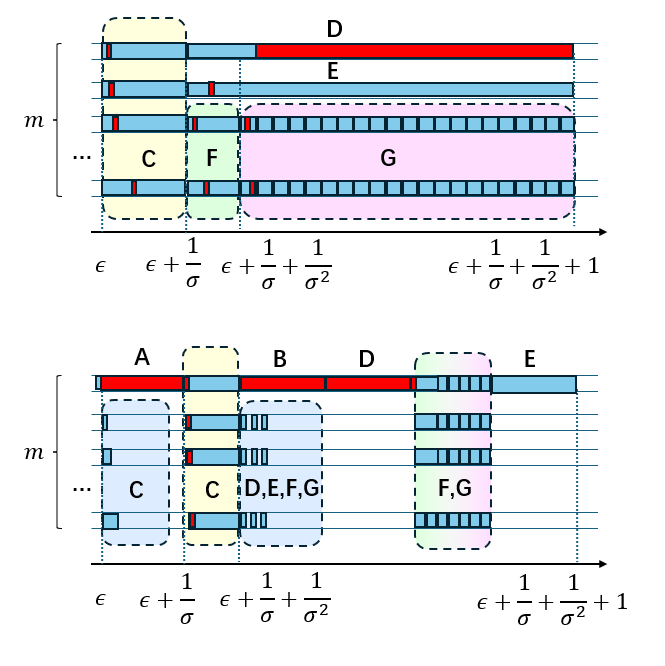
We first show that there is this set of jobs $J$ is feasible. The schedule is shown in Figure 4 on the top. $A$ and $B$ are scheduled at the very end since their deadline is much later (not shown in the figure). In time period $[\epsilon,\epsilon+1/\sigma]$ , group $C$ is released, and all $m$ jobs in this group are completed in $1/\sigma$ time; since the critical section lengths can be non-overlapping, they can run on all $m$ processors concurrently. At this time, group $D$ , $E$ , $F$ are released. In the interval $[\epsilon+1/\sigma,\epsilon+1/\sigma+1/\sigma^{2}]$ all $m-3$ jobs of $F$ are executed. In addition, job $E$ also completes its critical section. Finally, in interval $[\epsilon+1/\sigma+1/\sigma^{2},\epsilon+1+1/\sigma+1/\sigma^{2}]$ , all of $G$ and the remaining part of $D$ and $E$ are completed. $E$ has already completed its critical section and occupies one processor until its deadline. $D$ occupies another processor, but is executing its work before the start of its critical section. In the first $\epsilon m^{2}$ time, we only run the head of the jobs of $G$ (on $m-2$ processors) to complete all their critical sections. At this time $D$ can acquire the lock. The sum of the non-blocked work of $G$ is exactly the remaining time on $m-2$ processors.

We now show EDF-Block cannot meet all deadlines with $\sigma\leq 4.11$ for large $m$ .

At time $0$ , we only have $A$ and $B$ available, and $A$ has the earlier deadline. So EDF-Block runs $A$ and $B$ , and $A$ takes the lock after $\epsilon$ time steps. When group $C$ arrives, each of the jobs do a small amount of work and then they block (job 1 of group $C$ blocks after doing $\epsilon^{2}$ work, job 2 ofter $2\epsilon^{2}$ work and so on). After job $A$ finishes its critical section at time $\epsilon+1/\sigma$ , jobs of group $C$ get locks successively one after the other and then occupy all $m$ processors since they have the earliest deadlines. When all jobs of $C$ complete, $D, E$ and $F$ start running, but they do not immediately need a lock (group $C$ will complete $\Theta(\epsilon^{2})$ earlier, which is not enough for $D, E, F$ to acquire a lock), and they only occupy $m-1$ processors; therefore, job $B$ sneaks in and acquires the lock. Then $G$ is released, and $D, E, F, G$ run until they block. Once $B$ releases the lock, since they have the same deadline, $D$ takes the lock and the others wait. Then, all of the critical sections complete; but our algorithm runs $F, G$ before $E$ .

Consider $E$ ’s finish time, it is

\underbrace{1/\sigma}_{A}+\underbrace{1/\sigma^{2}}_{C}+\underbrace{1/\sigma}_% {B}+\underbrace{1/\sigma}_{D}+\underbrace{\frac{m-3}{m}(1/\sigma^{3})}_{F}+% \underbrace{\frac{m-2}{m}(1/\sigma)}_{G}+\underbrace{1/\sigma+1/\sigma^{3}}_{E% }-\Theta(m^{2})\epsilon

With enough large $m$ and enough small $\epsilon$ , it is equivalent to $5/\sigma+1/\sigma^{2}+2/\sigma^{3}$ . This work must be done before $E$ ’s deadline of $1+1/\sigma+1/\sigma^{2}$ , which solves to $\sigma\geq 4.1179\ldots$ . $\hfill\blacktriangleleft$

This lower bound demonstrates many of the difficulties that EDF-Block faces. In the feasible schedule, E runs continuously from release time to deadline. On the other hand, in EDF-Block, it experiences many sources of interference. The simplest one is the group G – which causes work blocking. Simply put, jobs in group G have the same absolute deadline as E, but occupy all the processors and prevent E from executing (due to arbitrary ordering by EDF for jobs with the same deadline). Working backwards, we now get to job D which causes interference due to internal blocking – that is, it gets the lock and blocks E. These two sources of interference are relatively intuitive and already imply a lower bound of $3$ since the duration of blocking due to both D and G is almost as long as the length of job E. Now we get to a more interesting case – job B causes external blocking – it has a later deadline than E and one would think that it can not interfere. However, before E even gets to its critical section, B sneaks in and gets the lock, thereby blocking E when it does get to its critical section. This gets us to the lower bound of $4$ ; in fact, if we look critically at the example from Theorem 8, these are the sources of blocking for job $y$ in that example as well.

To get above $4$ for the lower bound is surprising and counter-intuitive, however, since we seem to have accounted for all sources of interference already. To do this, we have jobs A and C. In the optimal scheduler, C completes before E is even released; therefore, it can not interfere with E. However, in EDF-Block, A (whose deadline is much later) sneaks in before C and blocks C (this is external blocking for C). Therefore, the work of C gets pushed into E’s interval causing additional interference for E.

The upper bound analysis of EDF-Block is challenging precisely because one must account for all these sources of delay.

4.3 Lower bound for EDF-Block on tasks

In this subsection, we consider scheduling of sporadic tasks. We show that EDF-Block requires speed augmentation of at least 4 to schedule all feasible task sets. First, let us understand why the lower bound for jobs does not automatically generalize to implicit-deadline sporadic tasks – this also provides intuition for why this proof is so complicated. In order to show this lower bound, we must construct a set of feasible tasks which are “difficult” for EDF-Block. The key point here that the tasks must be feasible – this means that the jobs released by the tasks must be feasible for any valid release sequence. For sporadic tasks, there are an infinite number of (potentially infinitely long) release sequences and some optimal scheduler should be able to schedule all of them. We must then show that there are at least some release patterns of these tasks that EDF-Block can not schedule without sufficient speed. Constructing a set of such feasible tasks is the challenging part of this proof.

Theorem 3.

EDF-Block requires at least 4 speed augmentation to schedule all feasible task sets.

Proof.

We consider the following task set. Recall that a task is a tuple with $(w_{i},b_{i},d_{i},t_{i})$ where the terms are work, critical section length, deadline and period, respectively. Let $Q=P(2P/\epsilon+1)$ .

$\blacksquare$

task $A$ : $(P,P,Q,Q)$ : This is a long job with a long critical section.
$\blacksquare$

task $B$ : $(P,\epsilon,P,Q)$ : This is a long job with a short critical section.
$\blacksquare$

task $C$ – there are $m^{2}$ copies of this one: $((m-2)P/m^{2},\epsilon,P,Q)$ : These are moderate jobs with short critical section.
$\blacksquare$

task $D$ – there are $P/\epsilon-(m^{2}+1)$ copies of this one $(\epsilon,\epsilon,P,Q)$ : These are short jobs with short critical sections.

We first show that task set is feasible – that is, all possible release sequences of jobs that can be generated by this task set can be scheduler by an optimal scheduler which knows everything about the tasks including release times of each job. For simplicity, assume that this scheduler gets to decide when the critical sections of each job occur. Consider each single period. There are $P/\epsilon$ tasks of type $B, C, D$ , and they all have deadline $P$ and period $Q$ . We can cut the release time to deadline interval of any job of task $A$ into $2P/\epsilon+1$ intervals. There will be at least one interval of length $P$ that does not interfere with any jobs in tasks $B, C, D$ . This means that the optimal scheduler can put the job in task $A$ in this free interval without influencing tasks $B$ , $C$ , $D$ .

OPT will first schedule task $D$ at the earliest time after a job is released and the lock is free. We notice that: in each consecutive $P$ time steps, there are always $(m^{2}+1)\epsilon$ steps where the lock is not taken by $D$ . We temporarily call them idle steps. Then, it schedules $B, C$ as if there are no critical sections, which is always feasible due to a simple proof by contradiction on the total work. Now, for each of the $m^{2}+1$ jobs (say job $i$ ), there are four cases:

1.

if it contains $\epsilon$ of the idle steps, OPT reserves $\epsilon$ of them for its critical section (so these $\epsilon$ steps are not idle);
2.

if it does not contain enough idle steps, but $\epsilon$ of the idle steps are not fully filled (all the $m$ processors are full), then OPT moves $\epsilon$ of the work to these steps, and marks them as critical section;
3.

if it does not contain enough idle steps, and most of the idle steps are fully filled, then there must be enough work in the idle steps that are from task $C$ and are not in the critical section. If $\epsilon$ of these work from task $C$ shares the same life cycle with job $i$ , then OPT switches these work with job $i$ ’s work, and marks job $i$ ’s work as its critical section;
4.

finally, if most of the work do not share the same life cycle with job $i$ , this means there are more than $P$ available time steps, and these work could be moved elsewhere (or multiple moves in a chain). Job $i$ ’s work could be moved here and marked as critical section.

The worst case is that all the jobs from tasks $B, C, D$ has the same release time. In this case, the $m^{2}+1$ idle steps are just enough for the $m^{2}+1$ jobs of tasks $B, C$ , and the total work of all the jobs sums up to $P$ .

Now we show that EDF-Block can not schedule at least some release sequences of these tasks without sufficient speed. For EDF-Block, $A$ arrives and other jobs arrive soon after. $A$ will finish at time $P/\sigma$ . Then we execute all of $D$ finishing at time $P/\sigma-(m^{2}+1)\epsilon/\sigma$ . At this time, we can do all jobs in $C$ – even not worrying about blocking, this takes $(m-2)P/(m\sigma)$ time. Finally, $B$ takes $P/\sigma$ time. Therefore, we need

\underbrace{P/\sigma}_{A}+\underbrace{P/\sigma-(m^{2}+1)\epsilon/\sigma}_{D}+% \underbrace{(m-2)P/(m\sigma)}_{C}+\underbrace{P/\sigma}_{B}\leq P

which solves to $\sigma\geq 4$ assuming large $m$ and very small $\epsilon$ . $\hfill\blacktriangleleft$

5 An Upper Bound for EDF-Block

In this section, we will show that EDF-Block can schedule all feasible jobs with speed augmentation of $6$ . Since it is difficult to determine exact feasibility of jobs, we will compare EDF-Block to necessary (but not sufficient) conditions for feasibility. We will assume that a hypothetical scheduler, OPT, can schedule all sets of jobs that satisfy these conditions. ²²2Note that this OPT is sometimes not a real scheduler since our conditions are only necessary, but not sufficient; therefore, this OPT is slightly different from the OPT in the previous section. We will then define some terms that bound how far behind EDF-Block can be relative to this hypothetical scheduler given $\sigma$ speed augmentation. We will finally bound $\sigma$ by using structural properties of EDF-Block.

5.1 Feasibility Conditions

We start our proof by summarizing the necessary conditions that any feasible set of jobs must satisfy. We will compare against a scheduler that can potentially schedule all sets of jobs that satisfy these constraints. Let’s call this hypothetical scheduler OPT – such a scheduler may not exist since these conditions are not sufficient. However, we will prove that EDF-Block can schedule any set of jobs with speed 6 if they meet these conditions. The following claim is a direct corollary from Definition 3.

Claim 1 (Feasibility Conditions).

For any interval $[t,t^{\prime}]$ such that $T=t^{\prime}-t$ , say $X$ is the set of jobs which are released and have a deadline within this interval. Then, a feasible job set must satisfy the following conditions – otherwise, no scheduler can schedule these jobs and meet all deadlines.

1.

Each individual job can be scheduled within the interval. That is, for all $j\in X$ , $w_{j}\leq T$ .
2.

The total work that must be completed within the interval is feasible. That is:

$\sum_{j\in X}w_{j}\leq mT$
3.

The total critical section length of all the jobs combined is feasible. That is:

$\sum_{j\in X}b_{j}\leq T$

Recall that the jobs may not be feasible even if these conditions are true – so these are not sufficient, only necessary. However, the set of feasible jobs is a subset of jobs that satisfy these conditions. Therefore, an upper bound based on these conditions also applies to all job sets that are actually feasible.

5.2 Technical Overview and Intuition

Since this proof is somewhat complex, we will now provide some intuition on how we construct the proof. Consider a particular job, say job $J_{i}$ that has release time $r_{i}$ , work $w_{i}$ , critical section length $b_{i}$ and relative deadline $d_{i}$ . Note that in the worst case, $w_{i}=d_{i}$ ; so for the purposes of this proof, let us assume that. Now consider the various sources of interference that prevent this job from executing. First, it may be prevented from executing since all processors are busy executing higher priority jobs. Second, it may be blocked since a higher priority job holding the lock and this job is waiting on the lock. Third, it may be blocked by a lower priority job since this lower priority job got the lock and then our job $J_{i}$ reached its critical section.

In this proof, we will define an interval of interest – intuitively, this interval of interest should begin when EDF is ahead relative to OPT and ends at the deadline of job $J_{i}$ . However, for technical reasons, this definition of the start time is a little bit more complicated. Regardless, once we define this interval of interest, we divide this interval into segments of size $d_{i}$ . The reason for this division is that we can make arguments about progress in each of these intervals. In particular, pessimistically, we assume that all jobs that arrive within this interval do not make any progress within the interval. However, for all jobs that arrive before this interval, we can make some progress guarantees within each of these intervals via an induction argument.

The progress argument works as follows. We define lag as a quantity that encapsulates how far behind EDF-Block can be relative to OPT on any job. Intuitively, if the lag is small, then EDF-Block has made as much progress as OPT on all jobs (of interest). The induction argument says that either the lag at the end of the segment was small, or a lot work or critical sections were executed during the segment. This might seem counter-intuitive – one would imagine that doing a lot of work would contribute to smaller lag. However, note that lag is a quantity defined over all jobs – so if the processors are busy doing a lot of work and critical sections, then some jobs may lag even if, overall, a lot of progress is being made.

This leads us to the last segment once our job of interest $J_{i}$ is released. Due to the progress arguments, we realize that either EDF-Block has small lag or a lot of work and critical sections were executed already. This allows us to bound the amount of interference that job $J_{i}$ experiences.

5.3 Setup and the Interval of Interest

We want to calculate the speed augmentation needed by EDF-Block to guarantee schedulability. We will proceed by saying that EDF-Block has speed augmentation of $\sigma$ and then we will calculate $\sigma$ .

In order to do so, we consider a single job, say job $J_{i}$ and argue that this job will meet its deadline as long as the speed is at least $\sigma$ . Since this statement will hold for every generic job; this is sufficient to guarantee that all jobs will meet deadlines. For $J_{i}$ , we will say the release time $R=r_{i}$ , the deadline $F=r_{i}+d_{i}$ , and $d=d_{i}=F-R$ . We first define some subsets for relevant sets of jobs relative to our job under consideration, namely $J_{i}$ .

Definition 8 ( $X_{before},X_{after},\texttt{alive}(t)$ ).

Let the set $X_{before}$ contain jobs that have deadline³³3If there are multiple jobs with the same deadline, we assume that EDF prioritizes them arbitrarily. before or equal to $F$ , and let the set $X_{after}$ contain jobs that have deadline after $F$ . At any time $t$ , $\texttt{alive}(t)$ is the set of jobs in $X_{before}$ that have been released, but have not completed executing at this time.

Note that $J_{i}$ is in $X_{before}$ . Also, jobs in set $X_{after}$ can not interfere with the jobs in set $X_{before}$ except if they are holding the lock. Next, we define some notation to compare the progress made by EDF-Block and OPT on particular OPT is a hypothetical scheduler that can schedule all job sets that satisfy the conditions stated in Claim 1 and Definition 2.

Definition 9 ( $p_{j}(t),p^{*}_{j}(t),\texttt{jlag}(j,t)$ ).

For a job $J_{j}\in X$ , and at a particular time $t$ , we say $p_{j}(t)$ is the amount of work done by job $J_{j}$ at time $t$ under EDF-Block and $p^{*}_{j}(t)$ is the amount of work done by $J_{i}$ under OPT. At time $t$ , we say $\texttt{jlag}(j,t)=p^{*}_{j}(t)-p_{j}(t)$ .

In other words, $\texttt{jlag}(j,t)$ represents how much EDF-Block is “behind” on the job $J$ at time $t$ . If the jlag is negative, then EDF-Block is ahead on the job at time $t$ . By definition, if a job has not arrived yet, or has completed, then jlag for that job is $0$ .

These definitions now allow us to define our interval of interest. This interval of interest ends at time $F$ (the deadline of the job $J_{i}$ ) and starts at some time before $R$ (the release time of $J_{i}$ ). Intuitively, this interval should consist of the intervals of all jobs which can have an impact on the schedule of $J_{i}$ either by directly interfering with $J_{i}$ or by causing another job to interfere with $J_{i}$ . In principle, this interval could start at time $0$ , but could also start later.

To define this interval, imagine that we step backward from time $F$ and divide time into segments of size $d$ .

Definition 10 (Time segments).

Based on the relative deadline $d$ of job $J_{i}$ , the timeline before $F$ is divided into segments of size $d$ . Formally, the segments are $[R-kd,R-(k-1)d],\ldots,[R-d,R],[R,F]$ (where $k$ can be any integer greater than $0$ and will be defined soon). For a given $k$ , there are segments $0,1,\ldots,k$ , and segment $\ell$ starts at

t_{\ell}=R-kd+\ell d

for $\ell=0,1,\ldots,k$ . Specially, the last interval starts at $t_{k}=R$ , the release time of the job under consideration, namely $J_{i}$ .

For large enough $k$ , these time segments will cover the earliest release time $\min\{r_{j}\}$ , and nothing will run on the processor before it. For the purpose of this proof, we are interested in a particular interval which is defined by a value of $k$ such that $t_{0}$ for that $k$ to $F$ is our interval of interest.

Definition 11 ( $\texttt{lag}(t_{\ell})$ , $t_{s}$ ).

Let $t_{s}$ be the latest of these instants (the start of segments) such that $\texttt{jlag}(j,t_{s})\leq 0$ for all jobs $J_{j}$ which arrived at or before $t_{s-1}$ . That is, at time $t_{s}$ , EDF-Block has done at least as much work as OPT on all jobs that arrived before the previous segment. Formally,

\texttt{lag}(t_{\ell})=\max_{j\in\texttt{alive}(t_{\ell-1})}\{\texttt{jlag}(j,% t)\}

and

s=\max_{\texttt{lag}(t_{s})\leq 0}\{s\}

Note an important fact about this definition – the definition of lag at the start of a particular interval only considers jobs that were released before the start of the previous interval. It does not say anything about jobs that were released during the previous interval. Since no jobs are released before time $0$ , the start time of the first segment after time $0$ definitely satisfies this property. Therefore, $t_{s}$ is well defined. Since we do not care about any segments before $t_{s-1}$ , we will re-number $k$ such that $t_{s-1}=t_{0}$ and $t_{s}=t_{1}$ and subsequent segments accordingly. Note that $t_{s}$ could be equal to $R$ if this property is satisfied at time $R$ (in this case, $k=1$ ).

Corollary 1.

For the re-numbered $k$ and $1<\ell\leq k$ , $\texttt{lag}(t_{\ell})>0$ , and $\texttt{lag}(t_{1})\leq 0$ .

Within any segment of length $d$ within our interval of interest from $t_{s}$ to $F$ , we define progress as the minimum work done by EDF-Block on any job that was alive throughout the segment. Total progress is the sum of progress up to the end of segment $\ell$ .

Definition 12 ( $\texttt{prog},\texttt{tprog}$ ).

Denote time segment $[t_{\ell},t_{\ell+1}]$ as $s_{\ell}$ , we say

\texttt{prog}(s_{\ell})=\min_{i\in\texttt{alive}(t_{\ell})\cup\texttt{alive}(t% _{\ell+1})}\left\{p_{i}(t_{\ell+1})-p_{i}(t_{\ell})\right\}.

At the end of any segment $\ell$ , we define

\texttt{tprog}(t_{\ell+1})=\sum_{j=1}^{l}\texttt{prog}(s_{\ell}).

In short, within time segment $[t_{l},t_{\ell+1}]$ , all the jobs in $X_{before}$ should have at least $\texttt{prog}(s_{\ell})$ progress if they are alive. tprog is a more complicated concept and hard to define intuitively, but it quantifies how well EDF-Block is doing overall from $t_{s}$ to the end of a current interval.

5.4 Types of Time Steps

We will now classify each time step within the interval of interest as one of 4 types. (We use the example in Theorem 2 shown in Table 1 and Figure 4 to illustrate the various kinds of time steps. Let the only job in group $E$ be the selected $J_{i}$ .) Each time step is classified as one of the following:

Work step.: At least $m-1$ processors are working on jobs from $X_{before}$ , but are not executing their critical section. The time steps when group $C, F, G$ are working are work steps. In these steps, all of the $m$ processors are working, however, some time steps when only $m-1$ were doing so would also satisfy this condition.
Internal block (ib) step.: Some job from $X_{before}$ is holding the lock. The time steps when group $D$ takes the lock are examples of ib steps, since $D$ has an earlier deadline than our job of interest $E$ .
External block (eb) step.: Some job from $X_{after}$ is holding the lock. The time steps when group $B$ takes the lock are eb steps, since $B$ is in $X_{after}$ , but it takes the lock potentially blocking $E$ .
Incomplete step.: Matches none of the above. The time steps when group $E$ itself works (and is not executing its critical section) are incomplete steps, since all other $m-1$ processors are idle.

These four types of time steps cover possible types of steps; some steps may satisfy more than one condition, however. If this happens, we pick the earliest one. This means as long as $m-1$ processors are working without taking the lock, it is specified as a work step, and it does not matter if someone else is holding the lock.

Now we define terminology to count these steps within a certain interval.

Definition 13 ( $\texttt{w},\texttt{ibl},\texttt{ebl},\texttt{incomp}$ ).

Let $\texttt{w}(t,t^{\prime})$ be the number of work steps within time $[t,t^{\prime}]$ , $\texttt{ibl}(t,t^{\prime})$ be the number of ib steps, $\texttt{ebl}(t,t^{\prime})$ be the number of eb steps and $\texttt{incomp}(t,t^{\prime})$ be the number of incomplete steps.

5.5 Structural Properties of EDF-Block

We now prove some structural properties maintained by EDF-Block. In particular, we argue that jobs make a lot of progress on incomplete steps (and external blocking steps, to a more limited extent).

Lemma 1.

Given time interval $[t,t^{\prime}]$ before $F$ , and job $J_{j}$ in $X_{before}$ with release time $t$ or earlier. If $J_{j}$ is alive at $t^{\prime}$ , it makes progress on every incomplete step, i.e., it executes on every incomplete step increasing its $p_{j}(t)$ by $1$ .

Proof.

From the definition, no job is holding a lock (therefore, no one is blocked on the lock), and not all $m$ processors are working on jobs from set $X_{before}$ . Therefore, under EDF-Block, all jobs from $X_{before}$ which are alive will run. $\hfill\blacktriangleleft$

Now consider eb steps and argue that jobs in $X_{before}$ make progress on most eb steps while they are alive.

Lemma 2.

Say a time interval $[t,t^{\prime}]$ within our interval of interest from $t_{s}$ to $F$ , had $\texttt{ebl}(t,t^{\prime})$ external blocking steps. Any job $J_{j}$ in $X_{before}$ that was alive from $t$ to $t^{\prime}$ will make at least $\texttt{ebl}(t,t^{\prime})-d$ progress. That is, it will execute on all external blocking steps except perhaps $d$ of them.

Proof.

During external blocking steps, some job from $X_{after}$ holds the lock. Since all jobs from $X_{after}$ have deadline after $F$ , if they are alive at any time between $t$ and $t^{\prime}$ they must overlap with job $J_{i}$ . Therefore, their critical section length $b_{i}\leq d$ due to Definition 2.

We now argue that job $J_{j}$ which belongs to $X_{before}$ can be blocked at most once by a job in $X_{after}$ . Say some job $J_{p}$ in $X_{after}$ is holding the lock and this is an external blocking step. If $J_{j}$ is running, then it makes progress on this step. If $J_{j}$ is not running, this means that at least one processor is idle or is running another job $J_{q}$ from $X_{after}$ – recall that work step is defined as $m-1$ jobs from $X_{before}$ are running. Since $J_{j}$ is alive, the only reason it doesn’t run on this external blocking step is because it is waiting on the lock. However, once this job $J_{p}$ releases the lock, $J_{j}$ will acquire it before any other job from $X_{after}$ can acquire it since $J_{j}$ has higher priority for getting locks than any job in $X_{after}$ . Therefore, $J_{j}$ can be blocked by at most one job in $X_{after}$ for at most $d$ time. On all other eb steps, $J_{j}$ must run and make progress. $\hfill\blacktriangleleft$

To sum up, if there are enough eb steps and incomplete steps, there will be progress on all jobs that are alive. We will now use these properties to bound the number of work steps and the number of internal blocking steps.

We now move on to work steps and internal blocking steps. We must first consider work inside and outside critical sections separately and bound the amount of work done by OPT within a particular interval.

Lemma 3.

Within any time interval $[t,t^{\prime}]$ , and a subset of job $J^{\prime}$ , OPT does $W$ work which is outside critical sections and $I$ work which is within critical sections. Then, we have

\frac{1}{m-1}W+I\leq 2(t^{\prime}-t)

Proof.

The feasibility conditions in Claim 1 show that $I\leq t^{\prime}-t$ and $W+I\leq m(t^{\prime}-t)$ . Therefore,

\frac{1}{m-1}W+I=\frac{1}{m-1}(W+I)+\frac{m-2}{m-1}I\leq\frac{m+m-2}{m-1}(t^{% \prime}-t)=2(t^{\prime}-t)\

$\hfill\blacktriangleleft$

We now use this lemma to bound the number of work and internal blocking steps for our interval of interest which is from $t_{s}=t_{1}$ to $F$ . Recall that $t_{s}=t_{1}=F-kd$ is defined in Definition 11.

Lemma 4.

$\texttt{w}(t_{1},F)+\texttt{ibl}(t_{1},F)\leq 2(k+1)d$ .

Proof.

Define $J_{1}$ as the set of jobs in $X_{before}$ that were released before $t_{0}=F-(k+1)d$ and $J_{2}$ be the set of jobs in $X_{before}$ which were released after $t_{0}$ . Within interval $[t_{1},F]$ for $J_{1}$ (cumulatively), say OPT processes $W_{1}^{*}$ work outside the critical sections and $I_{1}^{*}$ work within the critical sections. Similarly define $W_{2}^{*},I_{2}^{*}$ for $J_{2}$ . Also, define similar quantities for EDF-block for $J_{1},J_{2}$ as $W_{1},I_{1},W_{2},I_{2}$ correspondingly.

From Lemma 3 on the whole $X_{before}$ , we know that

\frac{1}{m-1}(W_{1}^{*}+W_{2}^{*})+I_{1}^{*}+I_{2}^{*}\leq 2(F-t_{1})=2kd

Now consider EDF-Block. According to Definition 11, at $t_{1}$ , EDF-Block is ahead of OPT on all jobs released before $t_{0}$ (all of $J_{1}$ ); meanwhile, OPT completes them at time $F$ . Therefore, EDF-Block has less work to do on these jobs than OPT does; therefore $W_{1}\leq W_{1}^{*}$ , $I_{1}\leq I_{1}^{*}$ .

Now consider jobs in $J_{2}$ and consider time $t_{1}$ . At this time, the jobs released after $t_{1}$ have made equal progress in OPT and EDF-Block (namely 0). For jobs released between $t_{0}$ and $t_{1}$ , OPT has done at most $d$ work on them cumulatively within their critical sections in interval $[t_{0},t_{1}]$ , since $t_{1}-t_{0}=d$ . Therefore, $I_{2}\leq I_{2}^{*}+d$ . In the same way, counting the total work both inside and outside critical sections, we will get $W_{2}+I_{2}\leq W_{2}^{*}+I_{2}^{*}+md$ . This solves to

\frac{1}{m-1}W_{2}+I_{2}\leq\frac{1}{m-1}W_{2}^{*}+I_{2}^{*}+2d

Therefore, we get

\frac{1}{m-1}(W_{1}+W_{2})+(I_{1}+I_{2})\leq\frac{1}{m-1}(W_{1}^{*}+W_{2}^{*})% +(I_{1}^{*}+I_{2}^{*})+2d\leq 2(k+1)d

Finally, within the interval $[t_{1},F]$ , the $i b$ steps must contribute to $I_{1}$ or $I_{2}$ , so $\texttt{ibl}(t_{1},F)\leq I_{1}+I_{2}$ . Also, the $w o r k$ steps must contribute to $W_{1}$ or $W_{2}$ with $m-1$ processors, so $(m-1)\texttt{w}(t_{1},F)\leq W_{1}+W_{2}$ . This completes the proof. $\hfill\blacktriangleleft$

5.6 Bounds on Progress

We now get to the crucial proof in this paper – this proof is an inductive proof that relates the lag and tprog. That is, either no job is too far behind OPT or we haven’t made much progress.

Lemma 5.

At the end of interval $\ell$ , $\texttt{lag}(t_{\ell+1})\leq 2\ell d-\texttt{tprog}(t_{\ell+1})$ .

Proof.

We will show this by induction for $\ell=1,2,\ldots,k-1$ .

Base Case (for $\ell=1$ ).

Consider segment $s_{1}=[t_{1},t_{2}]$ . By definition of $\texttt{prog}(s_{1})$ , EDF-Block does at least $\texttt{prog}(s_{1})$ work on all jobs that were alive throughout the segment. At time $t_{1}$ , for any job $j$ that arrived before time $t_{0}$ , we have $\texttt{jlag}(j,t_{1})\leq 0$ by Definition 11. For these jobs, EDF-Block did at least $\texttt{prog}(s_{1})$ work during this segment. OPT made at most $d$ progress on these jobs. Therefore, at time $t_{2}$ , we have $\texttt{jlag}(j,t_{2})\leq d-\texttt{prog}(s_{1})$ . On the other hand, for a job $j$ that arrived between time $t_{0}$ and $t_{1}$ , OPT may do at most $2d$ work during the interval $[t_{0},t_{2}]$ . Therefore, the $\texttt{jlag}(j,t_{2})\leq 2d-\texttt{prog}(s_{1})$ .

Inductive Case.

Assume that after the $(\ell-1)$ -th segment, we have $\texttt{lag}(t_{\ell})\leq 2(\ell-1)d-\texttt{tprog}(t_{\ell})$ . During segment $\ell$ , the work done by OPT on any job is at most $d$ and the total work done by EDF-Block on any job that is alive throughout the segment is at least $\texttt{prog}(t_{\ell+1})$ by definition of prog.

Again, there are two cases. First, consider jobs that were released before $t_{\ell-1}$ – that is, they were also alive throughout the previous segment. These jobs counted towards the lag in the previous segment. Therefore, by the inductive hypothesis, we know that $\texttt{jlag}(j,t_{\ell})\leq\texttt{lag}(t_{\ell})\leq 2(\ell-1)d-\texttt{% tprog}(t_{\ell})$ . Therefore, since OPT does at most $d$ work and EDF-Block does at least $\texttt{prog}(s_{\ell})$ work, we have $\texttt{jlag}(j,t_{\ell+1})\leq 2(\ell-1)d-\texttt{tprog}(t_{\ell})+d-\texttt{% prog}(s_{\ell})\leq 2\ell d-\texttt{tprog}(t_{\ell+1})$ .

Now consider jobs that were released during the previous segment – $[t_{\ell-1},t_{\ell}]$ . These jobs were not included in the $\texttt{lag}(t_{\ell})$ . For these jobs, OPT does at most $2d$ work between time $t_{\ell-1}$ and $t_{\ell+1}$ and EDF-Block does work at least $\texttt{prog}(s_{\ell}$ during the $\ell$ -th segment. Therefore, $\texttt{jlag}(j,t_{\ell+1})\leq 2d-\texttt{prog}(s_{\ell})$ . Since $\texttt{lag}(t_{\ell})\geq 0$ , we further know that $\texttt{jlag}(j,t_{\ell+1})\leq 2d-\texttt{prog}(s_{\ell})+\texttt{lag}(t_{% \ell})\leq 2\ell d-\texttt{tprog}(t_{\ell+1})$ . $\hfill\blacktriangleleft$

The following corollary follows from the fact that lag is positive at the end of each interval.

Corollary 2.

At the end of any interval $\ell$ , $\texttt{tprog}(t_{\ell+1})\leq 2\ell d-\texttt{lag}(t_{\ell+1})\leq 2\ell d$ .

We now argue that either a segment has a lot of work or internal blocking steps or all jobs in $X_{before}$ make a lot of progress.

Lemma 6.

During any segment of size $d$ , we have

\texttt{w}(s_{l})+\texttt{ibl}(s_{l})+\texttt{prog}(s_{l})\geq(\sigma-1)d.

Proof.

Consider any job that was alive during the entire interval. Say there were $x$ steps during the interval which were either incomplete or eb. From Lemma 1 and Lemma 2, this job must make at least $\max\{x-d,0\}$ progress during this interval since it can be blocked only for $d$ steps total due to external blocking. Since there are a total of $\sigma\times d$ steps during this interval, the job must make progress at least $\sigma\times d-\texttt{w}(s_{k})-\texttt{ibl}(s_{k})-d$ , which gives us the result. $\hfill\blacktriangleleft$

This lemma may seem to be counter-intuitive – one might imagine that many work steps contribute to progress and not detract from progress. However, recall the peculiar definition of prog – it is the minimum progress over all jobs. On work steps, all processors may be busy, and therefore, some jobs in $X_{before}$ may not make progress. Similarly on internal blocking steps, some jobs from $X_{before}$ may not make progress. Only incomplete and external blocking steps (to a more limited extent) ensure that all jobs from $X_{before}$ are running.

We have a bound that relates work, ibl and prog. However, what we really need is to show that there are many work and internal blocking steps given sufficient speed augmentation. The following lemma shows the way to remove prog.

Lemma 7.

With speed $\sigma$ , during any interval $[t_{1},t_{l+1}]$ where $t_{l+1}$ is the end point of the segment $s_{l}$ , there are at least $(\sigma-3)ld$ steps which are either work or ib.

Proof.

From Corollary 2, we have

\texttt{tprog}(t_{l+1})\leq 2\ell d.

From Lemma 6, we have

\sum_{j=1}^{l}(\texttt{w}(s_{j})+\texttt{ibl}(s_{j}))\geq(\sigma-1)ld-\texttt{% tprog}(t_{l})\geq(\sigma-3)ld.\

$\hfill\blacktriangleleft$

5.7 Analysis of the last segment

Now we are prepared to finally compute $\sigma$ . Recall that we are considering a particular $J_{i}$ and want to argue that this job will meet its deadline with speed $\sigma$ . We have now shown that, given large enough $\sigma$ , a lot of work and internal blocking has been completed at the time when $J_{i}$ is released. We now consider the last segment that goes from the release time of $J_{i}$ , namely $R$ to its deadline, namely $F$ .

Theorem 4.

$\sigma=6$ speed augmentation is enough for EDF-Block to guarantee that all jobs will meet their deadlines for job systems which satisfy the feasibility conditions (from Claim 1) and limited blocking assumption (Definition 2).

Proof.

To prove this theorem, we bound $\texttt{w}(R,F)+\texttt{ibl}(R,F)$ . According to Lemma 4, we know that the total possible work and ib during the time interval from $[t_{1},F]$ is at most $2(k+1)d$ .

When $k=1$ , we have $R=t_{1}$ , and this is $4d$ .

When $k\geq 2$ , from Lemma 7 with $l=k-1$ , at time $R$ , $(\sigma-3)(k-1)d$ work and ib steps have completed. Therefore, the work and ib steps that must execute within interval $[R,F]$ are

	$\displaystyle\texttt{w}(R,F)+\texttt{ibl}(R,F)$	$\displaystyle=\texttt{w}(t_{1},F)+\texttt{ibl}(t_{1},F)-\texttt{w}(t_{1},R)-% \texttt{ibl}(t_{1},R)$
		$\displaystyle\leq 2(k+1)d-(\sigma-3)(k-1)d$
		$\displaystyle=(4-(\sigma-5)(k-1))d$

Therefore, when $\sigma\geq 5$ , $4d$ is always an upper bound for $\texttt{w}(R,F)+\texttt{ibl}(R,F)$ . This means $\texttt{ebl}(R,F)+\texttt{incomp}(R,F)\geq(\sigma-4)d$ . Using Lemma 1 and Lemma 2 on $J_{i}$ , there are at least $(\sigma-4)d-d=(\sigma-5)d$ time steps on which $J_{i}$ makes progress. Since the work $w_{i}$ of $J_{i}$ is at most its relative deadline $d$ , when $\sigma\geq 6$ , $J_{i}$ makes enough progress to complete. $\hfill\blacktriangleleft$

5.8 Generalization to Tasks

Now let us consider tasks. It is easy to see that the result also applies to tasks.

Corollary 3.

$\sigma=6$ speed augmentation is enough for EDF-Block to solve arbitrary blocked deadline scheduling problem on tasks.

Proof.

Consider a feasible set of tasks. A task set is feasible only if all (possibly infinite) sequences of jobs that can be generated by that task set are feasible. Any given sequence of jobs generated by a feasible task set must satisfy the feasibility conditions defined in Claim 1. Theorem 4 shows that for any job set that satisfies the feasibility conditions, EDF-Block can schedule the job set on processors of speed 4. Therefore, given any feasible task set, EDF-Block can schedule it on processors of speed 4. $\hfill\blacktriangleleft$

6 Experimental Evaluation

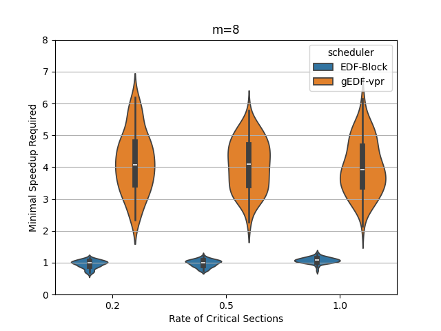
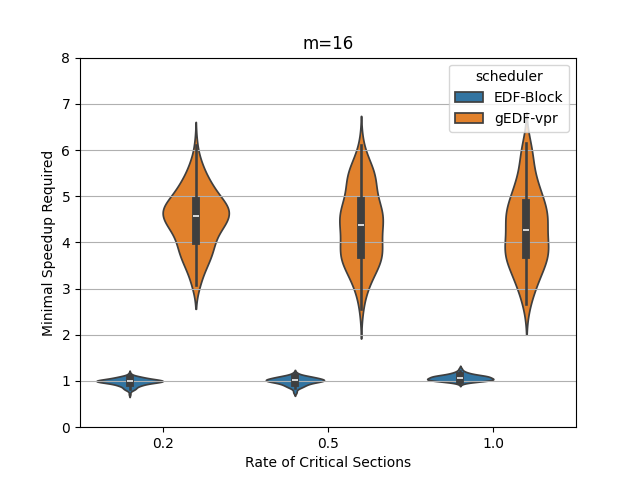
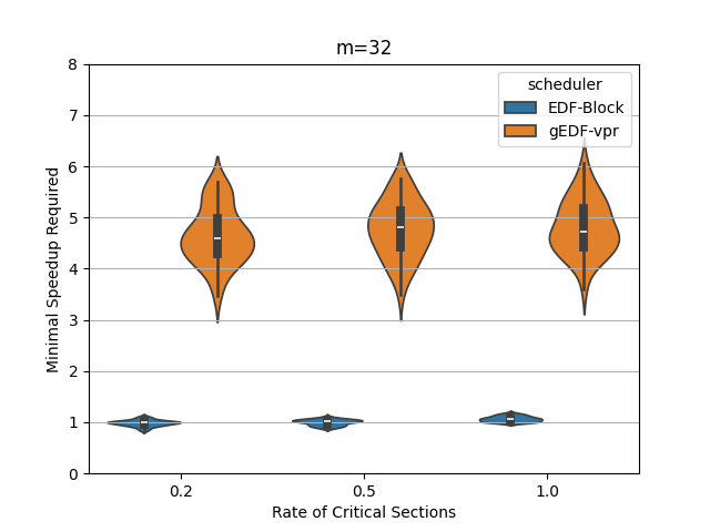
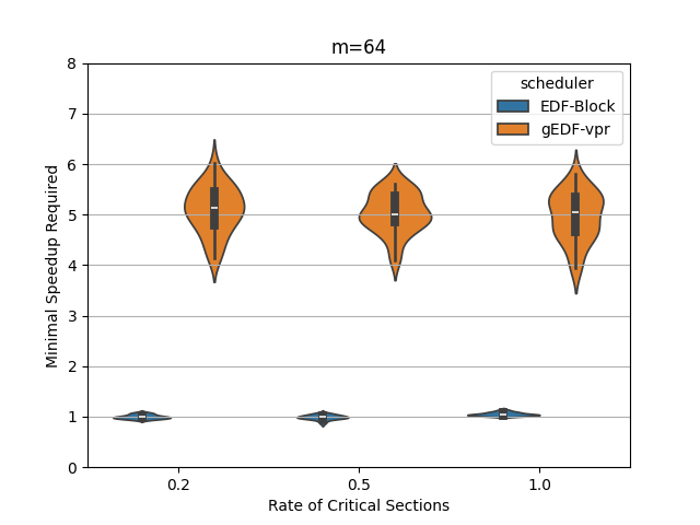
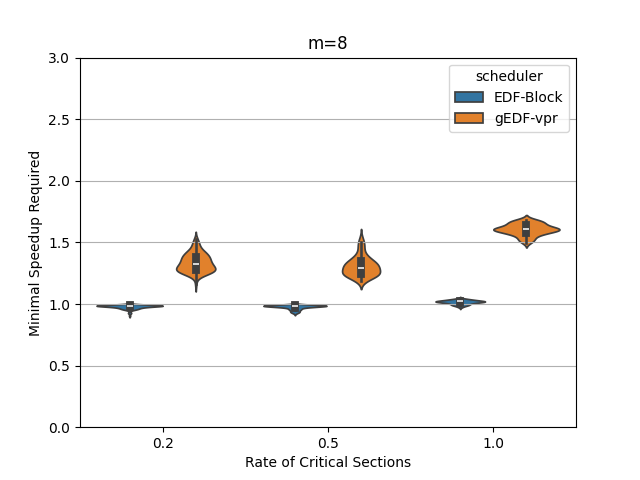
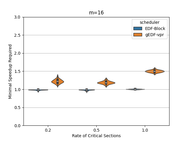
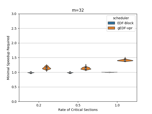
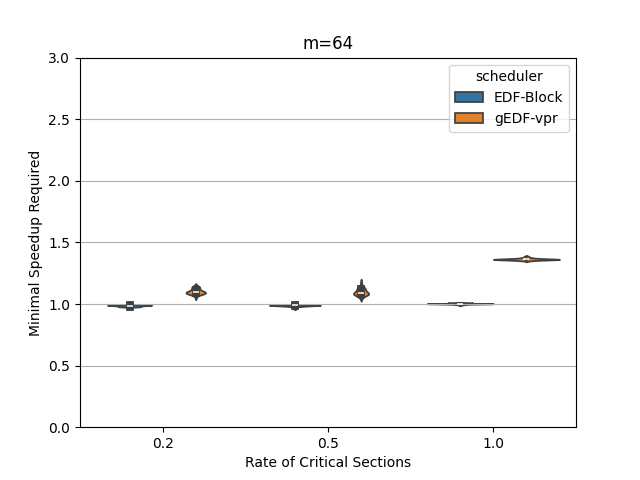
In this section, we perform an experimental evaluation of EDF-Block and compare it to gEDF-vpr [3]. gEDF-vpr is also an algorithm based on EDF for systems with resource sharing. We generate tasks randomly using the procedure similar to that in [11] for a variety of levels of contention and for various number of processors. We compare the speedup required to schedule the tasks using EDF-Block with that required by gEDF-vpr. Our experiments indicate that for these tasks, the speedup required is much smaller than the theoretical lower or upper bounds for both schedulers. In particular, the speedup required by EDF-Block is generally very close to 1, while the speedup required by gEDF-vpr is varies based on experimental parameters, but can be as high as 7 for some task parameters.

Algorithm gEDF-vpr

The algorithm gEDF-vpr is based on global-EDF, but uses virtual processors. It converts the problem of scheduling $n$ implicit deadline tasks on $m$ processors to a problem of scheduling $3n$ constrained deadline tasks on $2m+1$ virtual processors. Consider a task $\tau_{i}$ of the original task set with release time $r_{i}$ , computation time $w_{i}$ , blocking time $b_{i}$ and deadline $d_{i}$ . Each task $\tau_{i}$ is split into three subtasks – the computation before the critical section belongs to the first one, call it $\tau_{i}^{A}$ , the critical section belongs to the second one, called $\tau_{i}^{B}$ and the computation after the critical section belongs to the third one $\tau_{i}^{C}$ .

A job corresponding $\tau_{i}^{A}$ is released when the original job $\tau_{i}$ is released and has a relative deadline of $d_{i}/3$ ; a job corresponding to $\tau_{i}^{B}$ is released at an offset of $d_{i}/3$ from the original release time and has relative deadline $d_{i}/3$ (therefore, its relative deadline from the release time of $\tau_{i}$ is $2d_{i}/3$ ; and a job corresponding to $\tau_{i}^{C}$ is released at an offset of $2d_{i}/3$ from the original release time and has relative deadline $d_{i}/3$ . Essentially, the interval of each job is split into $3$ equal parts and each job is also split into three parts which execute within each of these partial intervals. $m$ processors are converted into $2m+1$ virtual processors (of lower speed) whereby jobs in $\tau^{A}$ and $\tau^{C}$ execute on $m$ processors (each) using preemptive EDF and the jobs in $\tau^{B}$ execute on $1$ processor using non-preemptive EDF.

Andersson et al. [3] showed that this scheduler provides a speedup upper bound of $12(1+R)$ where $R$ is the number of resources. Therefore, for the simple case of $1$ resource, the speedup bound is $24$ .

Task Generation and Simulation Settings

The task are generated with a similar method as [11]. We consider varying number of processors, namely $m\in\{8,16,32,64\}$ . The period $p_{i}$ of each task $i$ is uniformly random in $[10000,100000]$ , and the deadline of each task is equal to its period – so these are implicit deadline tasks. The work $w_{i}=u_{i}\cdot p_{i}$ of each task is decided by the utilization $u_{i}$ . We use two methods to decide the utilization $u_{i}$ of each task. In the exponential task set, where $u_{i}$ is exponentially random with a mean of $\bar{u}=0.25$ . Therefore, the average utilization of tasks is $0.25$ . We always generate $n=4m$ tasks; therefore, the total utilization is $m$ in expectation – therefore, the machine is expected to be fully loaded. In the uniform task set, the utilization $u_{i}$ is uniformly random in $[0.05,0.15]$ . Therefore, the mean utilization is $\bar{u}=0.1$ . In this case, the number of tasks $n=10m$ in this case – again, in expectation the total utilization is $m$ and the machine is fully loaded.

Finally, the critical section length $b_{i}$ is uniformly random in $[1,C]$ , where $C=55000\cdot\bar{u}\cdot B\cdot\frac{2}{m}$ . Here, $B\in\{0.2,0.5,1\}$ is the blocking rate – that is, it is a measure of contention in the system. When $B=0.2$ , then the blocking is small and increases is $B$ increases.

In addition, there are feasibility checks: as tasks are generated, if the total utilization reaches $m$ or the total blocking requirement is above $1$ , then no further tasks are added to the task set since no scheduler can schedule such task sets on speed 1 processors. Note that this does not imply that all task sets we check are actually feasible on speed 1 since some sets with lower utilization may still be infeasible. However, this is the simplest check for feasibility and allows us to compare the two schedulers fairly.

During the simulation, the first release of each task is randomly selected. The position of each critical section ( $s_{i}$ in definition) is also randomly selected in the work time. We generate $100$ task sets of each processor count. We run EDF-Block exactly as in this article. For gEDF-vpr, we assign $2m+1$ processors as if they are the virtual processors as described in the paper that proposed that scheduling strategy. For both algorithms, we apply binary search to find the minimal speedup that is required to schedule all tasks in the task set.

Experimental Results

Figures 5 and 6 show the experimental comparison when the utilization of tasks is generated randomly using an exponential and a uniform distribution respectively. The $x-axis$ shows the contention parameter $B$ – the first set is when $B=0.2$ , the second when $B=0.5$ , and the last when $B=1.0$ . The $y-axis$ shows the speedup required to schedule the task set meeting all deadlines. The width of the bubble shows the fraction of task sets that needed that speed.

The experiments indicate the EDF-Block performs unexpectedly well for these randomly generated task sets. Most of the task sets require almost no speedup at all and this seems relatively insensitive to the amount of blocking or to the number of processors.

When the utilization of tasks is uniformly generated (Figure 6, gEDF-vpr also performs quite well and generally requires a speedup of less than 2 and often quite close to $1$ . However, then the utilizations are generated exponentially, gEDF-vpr seems to require higher speedups, but still substantially lower than the theoretical upper bounds indicate. The experimental analysis indicates that the randomly generated task sets do not generally cause anything close to the worst case performance seen in the lower bounds.

7 Related Work

We now review some related work. The problem of scheduling tasks with deadlines and shared resources has been extensively studied in the real-time systems community and several strategies have been developed. However, most of this work does not consider speedup bounds. Here we review some of this work to draw comparison with our approach and then focus on related work that does consider speedup bounds.

Some of the early work on reducing the impact of locks and semaphores focuses on uniprocessor scheduling. One classic example is stack based resource allocation policy (SRP) [5]. Other classic early work focuses on reducing the priority inversion by designing protocols such as priority ceiling protocol and priority inheritance protocol [36, 31, 32, 17]. In these systems, the job holding the lock (that is, executing the critical section) may itself be preempted by higher priority jobs. These protocols are designed to minimize the impact of priority inversion under this setting. On uniprocessors, it is generally necessary to allow this kind of preemption; otherwise, lower priority jobs holding a lock can delay higher priority jobs that do not even require a lock. This priority ceiling and inheritance ideas have been extended to multiprocessors [32, 34, 13] and some of this work also considers nested critical sections, which we do not allow. Chen and Tripathi [13], for instance, analyze a priority ceiling protocol for clustered scheduling and provide a schedulability test. In our design, we assume that critical sections are themselves non-preemptive; therefore, there is no need for priority ceiling or priority inheritance.

There has been a significant amount of work on locking protocols for multiprocessors – see [8] for a survey. Most prior work on multiprocessor scheduling considers how to incorporate blocking into schedulability analysis by optimizing and then computing bounds on blocking time of jobs (for instance [39, 9, 12]). In particular, an interesting model of design and analysis has been to analyze the amount of priority inverted blocking (called pi-blocking) experienced by jobs – for instance, Brandenberg et al. [10, 11, 9, 7] design a family of protocols for partitioned, clustered and global schedulers which all guarantee $O(1)$ pi-blocking. This essentially means that each critical section can be locked by at most a constant number of critical sections of lower priority jobs. For context, our scheduler guarantees that pi-blocking is at most $1$ per critical section – so it is stronger than $O(1)$ pi-blocking. While $O(1)$ pi-blocking is certainly necessary to get any constant competitive bound, it is not in itself sufficient to prove a speedup bound.

There is a limited amount of work that considers scheduling with resource sharing with analysis in terms of speedup bounds [33, 3, 4]. The most related is by Andersson and Easwaran [3] which splits tasks into subtasks and then uses EDF with virtual processors. They get a speedup upper bound of $12(1+\rho)$ which is $24$ for a single resource. This is the scheduler we compare against in our experimental section. In later work and with more complicated schedulers, this speedup was improved to $4+6\rho$ [33]. To our knowledge, 10 is the existing best upper bound for our problem (as the special case for $\rho=1)$ . Another work by Andersson et al. [4] is on $t$ -type heterogeneous multiprocessor platform, and has the upper bound of $4\times(1+\lceil\frac{|R|}{\min\{m_{1},m_{2},\ldots,m_{t}\}}\rceil)$ when the number of resources is 1.

Scheduling with release times and deadlines for jobs (called the SRDM problem) [20] has been studied extensively without resource sharing. Although the offline version of SRDM is NP-complete, there are various speedup bounds for variations in models. Kao et al. [25] applies competitive analysis and has the lower and upper bound of 2.09 and 5.2. Devanur et al. [22] further achieves a tight bound of $e$ assuming uniform length of jobs. These results are for the non-preemptive jobs, but the problem is open when they are preemptive [23]. Chen et al. [14] summarize the results, ending in various constants based on different settings of the problem [18, 2, 16, 15]. Note that our problem is a mixture of non-preemptive (the critical section) and preemptive (everything else), so it is different from the normal SRDM problem.

Another way to think about our problem is to divide each job into three parts, the first part is the portion of work before the critical section, the second is the critical section, and the third is the portion of work after the critical section. Only the middle part would be non-preemptive. Berger et al. [6] proposed fixed order scheduling and analyzed the first-fixed algorithm. Critical sections can also be seen as constraints of the problems, like the interval constraints [19, 28]. Saha [35] proposed “Renting the Cloud” model which also places constraints on intervals of jobs. For such the interval scheduling problems [26] EDF has been considered and analysed [37, 21, 41]. None of this work directly applies to our problem. EDF and its variants have been analyzed for many real-time scheduling problems like pair relations [40], deadline inheritance [24], scheduling of parallel programs [27, 30], quantized deadlines [42], and multi-criticality systems [38, 1].

8 Conclusions

In this paper, we have provided both lower and upper bounds on speedup for EDF-Block, a simple and intuitive generalization of EDF which handles jobs and sporadic tasks with critical sections protected by locks. We consider a simple model here with a single shared resource and a single critical section per job. This serves as preliminary work towards a greater understanding of this problem as well as this simple scheduling strategy.

There are several directions for future work. First, and most obviously, there is a gap between the upper and lower bounds even for this simple model. Second, more general models with multiple locks and multiple critical sections per job might be considered. Finally, one could imagine generalizations of other schedulers such as partitioned EDF and various fixed priority schedulers. Some of these have been considered in the literature, but as far as we know, there isn’t much analysis for speedup bounds for real-time jobs and tasks with critical sections. For real-time scheduling theory, this appears to be a fruitful area of research which is underexplored.

While we state the result in this paper as a speedup factor, OPT we are comparing against is not an optimal algorithm, but more a feasibility test. In this sense, this bound is more like a capacity augmentation bound [27]. One can easily convert it to a schedulability test by checking if the total work and critical section length within any interval can exceed the feasible limits. However, given the strong lower bound of $4$ for speedup, one might also consider designing other, more sophisticated, schedulability tests for this simple scheduler which might still require speed 4 on some task sets but may do better on other task sets.

References

[1] Sebastian Altmeyer. A comparison between fixed priority and edf scheduling accounting for cache related pre-emption delays. LITES, 1, April 2014. doi:10.4230/LITES-v001-i001-a001.
[2] S. Anand, Naveen Garg, and Nicole Megow. Meeting deadlines: How much speed suffices? In International Colloquium on Automata, Languages and Programming, 2011. URL: https://api.semanticscholar.org/CorpusID:16885010.
[3] Björn Andersson and Arvind Easwaran. Provably good multiprocessor scheduling with resource sharing. Real-Time Systems, 46:153–159, October 2010. doi:10.1007/s11241-010-9105-6.
[4] Björn Andersson and Gurulingesh Raravi. Real-time scheduling with resource sharing on heterogeneous multiprocessors. Real - Time Systems, 50(2):270–314, March 2014. Real-Time Systems is a copyright of Springer, (2014). All Rights Reserved; 2023-12-03. doi:10.1007/S11241-013-9195-Z.
[5] T.P. Baker. A stack-based resource allocation policy for realtime processes. In [1990] Proceedings 11th Real-Time Systems Symposium, pages 191–200, 1990. doi:10.1109/REAL.1990.128747.
[6] Andre Berger, Arman Rouhani, and Marc Schroder. Fixed order scheduling with deadlines. arXiv preprint arXiv:2412.10760, 2024.
[7] Bjorn B. Brandenburg. Scheduling and locking in multiprocessor real-time operating systems. PhD thesis, The University of North Carolina at Chapel Hill, USA, 2011. AAI3502550.
[8] Björn B. Brandenburg. Multiprocessor real-time locking protocols: A systematic review. CoRR, abs/1909.09600, 2019. arXiv:1909.09600.
[9] Bjorn B. Brandenburg and James H. Anderson. Optimality results for multiprocessor real-time locking. In 2010 31st IEEE Real-Time Systems Symposium, pages 49–60, 2010. doi:10.1109/RTSS.2010.17.
[10] Björn B. Brandenburg and James H. Anderson. The omlp family of optimal multiprocessor real-time locking protocols. Des. Autom. Embedded Syst., 17(2):277–342, June 2013. doi:10.1007/s10617-012-9090-1.
[11] Björn B. Brandenburg. The fmlp+: An asymptotically optimal real-time locking protocol for suspension-aware analysis. In 2014 26th Euromicro Conference on Real-Time Systems, pages 61–71, 2014. doi:10.1109/ECRTS.2014.26.
[12] Alan Burns and A.J. Wellings. A schedulability compatible multiprocessor resource sharing protocol – mrsp. In 2013 25th Euromicro Conference on Real-Time Systems, pages 282–291, July 2013. doi:10.1109/ECRTS.2013.37.
[13] Chia-mei Chen and Satish Tripathi. Multiprocessor priority ceiling based protocols. Technical Report CS-TR-3252, March 2001.
[14] Lin Chen, Nicole Megow, and Kevin Schewior. New results on online resource minimization. arXiv preprint arXiv:1407.7998, 2014. arXiv:1407.7998.
[15] Lin Chen, Nicole Megow, and Kevin Schewior. An o(log m)-competitive algorithm for online machine minimization. In ACM-SIAM Symposium on Discrete Algorithms, 2015. URL: https://api.semanticscholar.org/CorpusID:8317885.
[16] Lin Chen, Nicole Megow, and Kevin Schewior. An o( $m^{2}$ log m)-competitive algorithm for online machine minimization. ArXiv, abs/1506.05721, 2015. arXiv:1506.05721.
[17] M. Chen and K. Lin. Dynamic priority ceilings: A concurrency control protocol for real-time systems. Real Time Systems, 2:326–346, 1990.
[18] Julia Chuzhoy and Paolo Codenotti. Erratum: Resource minimization job scheduling. In International Workshop and International Workshop on Approximation, Randomization, and Combinatorial Optimization. Algorithms and Techniques, 2009. URL: https://api.semanticscholar.org/CorpusID:2190162.
[19] Julia Chuzhoy, Sudipto Guha, Sanjeev Khanna, and Joseph Naor. Machine minimization for scheduling jobs with interval constraints. 45th Annual IEEE Symposium on Foundations of Computer Science, pages 81–90, 2004. doi:10.1109/FOCS.2004.38.
[20] Mark Cieliebak, Thomas Wilhelm Erlebach, Fabian Hennecke, Birgitta Weber, and Peter Widmayer. Scheduling with release times and deadlines on a minimum number of machines. In IFIP TCS, 2004. URL: https://api.semanticscholar.org/CorpusID:15017335.
[21] Robert I. Davis. A review of fixed priority and edf scheduling for hard real-time uniprocessor systems. SIGBED Rev., 11(1):8–19, February 2014. doi:10.1145/2597457.2597458.
[22] Nikhil R. Devanur, Konstantin Makarychev, Debmalya Panigrahi, and Grigory Yaroslavtsev. Online algorithms for machine minimization. ArXiv, abs/1403.0486, 2014. arXiv:1403.0486.
[23] Weiqiao Han and Karren D. Yang. Preemptive Online Machine Minimization, 2016. URL: https://api.semanticscholar.org/CorpusID:228102474.
[24] P.G. Jansen, Sape J. Mullender, Johan Scholten, and Paul J.M. Havinga. Lightweight EDF Scheduling with Deadline Inheritance. Number 2003-23 in CTIT-technical reports. Centre for Telematics and Information Technology (CTIT), Netherlands, May 2003. Imported from DIES.
[25] Mong-Jen Kao, Jian-Jia Chen, Ignaz Rutter, and Dorothea Wagner. Competitive design and analysis for machine-minimizing job scheduling problem. In International Symposium on Algorithms and Computation, 2012. URL: https://api.semanticscholar.org/CorpusID:14459222.
[26] Antoon W. J. Kolen, Jan Karel Lenstra, Christos H. Papadimitriou, and Frits C. R. Spieksma. Interval scheduling: A survey. Naval Research Logistics (NRL), 54, 2007. URL: https://api.semanticscholar.org/CorpusID:15288326.
[27] Jing Li, Zheng Luo, David Ferry, Kunal Agrawal, Christopher Gill, and Chenyang Lu. Global edf scheduling for parallel real-time tasks. Real-Time Systems, 51:395–439, 2015. doi:10.1007/S11241-014-9213-9.
[28] Luis Osorio-Valenzuela, Jordi Pereira, Franco Quezada, and Óscar C. Vásquez. Minimizing the number of machines with limited workload capacity for scheduling jobs with interval constraints. Applied Mathematical Modelling, 2019. URL: https://api.semanticscholar.org/CorpusID:182422789.
[29] Cynthia A. Phillips, Cliff Stein, Eric Torng, and Joel Wein. Optimal time-critical scheduling via resource augmentation (extended abstract). In Proceedings of the Twenty-Ninth Annual ACM Symposium on Theory of Computing, STOC ’97, pages 140–149, New York, NY, USA, 1997. Association for Computing Machinery. doi:10.1145/258533.258570.
[30] Manar Qamhieh, Frédéric Fauberteau, Laurent George, and Serge Midonnet. Global edf scheduling of directed acyclic graphs on multiprocessor systems. In Proceedings of the 21st international conference on real-time networks and systems, pages 287–296, 2013. doi:10.1145/2516821.2516836.
[31] R Rajkumar. Synchronization in Real-Time Systems A Priority Inheritance Approach. Springer, 1991.
[32] R. Rajkumar, L. Sha, and J.P. Lehoczky. Real-time synchronization protocols for multiprocessors. In Proceedings. Real-Time Systems Symposium, pages 259–269, 1988. doi:10.1109/REAL.1988.51121.
[33] Gurulingesh Raravi, Vincent Nélis, and Björn Andersson. Real-time scheduling with resource sharing on uniform multiprocessors. In Proceedings of the 20th International Conference on Real-Time and Network Systems, RTNS ’12, pages 121–130, New York, NY, USA, 2012. Association for Computing Machinery. doi:10.1145/2392987.2393003.
[34] Jim Ras and Albert M.K. Cheng. An evaluation of the dynamic and static multiprocessor priority ceiling protocol and the multiprocessor stack resource policy in an smp system. In 2009 15th IEEE Real-Time and Embedded Technology and Applications Symposium, pages 13–22, 2009. doi:10.1109/RTAS.2009.10.
[35] Barna Saha. Renting a cloud. In Foundations of Software Technology and Theoretical Computer Science, 2013. URL: https://api.semanticscholar.org/CorpusID:17196958.
[36] L. Sha, R. Rajkumar, and J.P. Lehoczky. Priority inheritance protocols: an approach to real-time synchronization. IEEE Transactions on Computers, 39(9):1175–1185, 1990. doi:10.1109/12.57058.
[37] John A Stankovic, Marco Spuri, Krithi Ramamritham, and Giorgio Buttazzo. Deadline scheduling for real-time systems: EDF and related algorithms, volume 460. Springer Science & Business Media, 1998.
[38] Hang Su, Dakai Zhu, and Scott Brandt. An elastic mixed-criticality task model and early-release edf scheduling algorithms. ACM Trans. Des. Autom. Electron. Syst., 22(2), December 2016. doi:10.1145/2984633.
[39] Alexander Wieder and Björn B. Brandenburg. On spin locks in autosar: Blocking analysis of fifo, unordered, and priority-ordered spin locks. In 2013 IEEE 34th Real-Time Systems Symposium, pages 45–56, 2013. doi:10.1109/RTSS.2013.13.
[40] Jia Xu and David Parnas. Scheduling processes with release times, deadlines, precedence and exclusion relations. IEEE Trans. Softw. Eng., 16(3):360–369, March 1990. doi:10.1109/32.48943.
[41] Fengxiang Zhang. Analysis for EDF Scheduled Real Time Systems. Department for Computer Science, University of York, 2009.
[42] HaiFeng Zhu, J.P. Hansen, J.P. Lehoczky, and R. Rajkumar. Optimal partitioning for quantized edf scheduling. In 23rd IEEE Real-Time Systems Symposium, 2002. RTSS 2002., pages 212–222, 2002. doi:10.1109/REAL.2002.1181576.

[bib.bib1] [1] Sebastian Altmeyer. A comparison between fixed priority and edf scheduling accounting for cache related pre-emption delays. LITES, 1, April 2014. doi:10.4230/LITES-v001-i001-a001.

[bib.bib2] [2] S. Anand, Naveen Garg, and Nicole Megow. Meeting deadlines: How much speed suffices? In International Colloquium on Automata, Languages and Programming, 2011. URL: https://api.semanticscholar.org/CorpusID:16885010.

[bib.bib3] [3] Björn Andersson and Arvind Easwaran. Provably good multiprocessor scheduling with resource sharing. Real-Time Systems, 46:153–159, October 2010. doi:10.1007/s11241-010-9105-6.

[bib.bib4] [4] Björn Andersson and Gurulingesh Raravi. Real-time scheduling with resource sharing on heterogeneous multiprocessors. Real - Time Systems, 50(2):270–314, March 2014. Real-Time Systems is a copyright of Springer, (2014). All Rights Reserved; 2023-12-03. doi:10.1007/S11241-013-9195-Z.

[bib.bib5] [5] T.P. Baker. A stack-based resource allocation policy for realtime processes. In [1990] Proceedings 11th Real-Time Systems Symposium, pages 191–200, 1990. doi:10.1109/REAL.1990.128747.

[bib.bib6] [6] Andre Berger, Arman Rouhani, and Marc Schroder. Fixed order scheduling with deadlines. arXiv preprint arXiv:2412.10760, 2024.

[bib.bib7] [7] Bjorn B. Brandenburg. Scheduling and locking in multiprocessor real-time operating systems. PhD thesis, The University of North Carolina at Chapel Hill, USA, 2011. AAI3502550.

[bib.bib8] [8] Björn B. Brandenburg. Multiprocessor real-time locking protocols: A systematic review. CoRR, abs/1909.09600, 2019. arXiv:1909.09600.

[bib.bib9] [9] Bjorn B. Brandenburg and James H. Anderson. Optimality results for multiprocessor real-time locking. In 2010 31st IEEE Real-Time Systems Symposium, pages 49–60, 2010. doi:10.1109/RTSS.2010.17.

[bib.bib10] [10] Björn B. Brandenburg and James H. Anderson. The omlp family of optimal multiprocessor real-time locking protocols. Des. Autom. Embedded Syst., 17(2):277–342, June 2013. doi:10.1007/s10617-012-9090-1.

[bib.bib11] [11] Björn B. Brandenburg. The fmlp+: An asymptotically optimal real-time locking protocol for suspension-aware analysis. In 2014 26th Euromicro Conference on Real-Time Systems, pages 61–71, 2014. doi:10.1109/ECRTS.2014.26.

[bib.bib12] [12] Alan Burns and A.J. Wellings. A schedulability compatible multiprocessor resource sharing protocol – mrsp. In 2013 25th Euromicro Conference on Real-Time Systems, pages 282–291, July 2013. doi:10.1109/ECRTS.2013.37.

[bib.bib13] [13] Chia-mei Chen and Satish Tripathi. Multiprocessor priority ceiling based protocols. Technical Report CS-TR-3252, March 2001.

[bib.bib14] [14] Lin Chen, Nicole Megow, and Kevin Schewior. New results on online resource minimization. arXiv preprint arXiv:1407.7998, 2014. arXiv:1407.7998.

[bib.bib15] [15] Lin Chen, Nicole Megow, and Kevin Schewior. An o(log m)-competitive algorithm for online machine minimization. In ACM-SIAM Symposium on Discrete Algorithms, 2015. URL: https://api.semanticscholar.org/CorpusID:8317885.

[bib.bib16] [16] Lin Chen, Nicole Megow, and Kevin Schewior. An o( $m^{2}$ log m)-competitive algorithm for online machine minimization. ArXiv, abs/1506.05721, 2015. arXiv:1506.05721.

[bib.bib17] [17] M. Chen and K. Lin. Dynamic priority ceilings: A concurrency control protocol for real-time systems. Real Time Systems, 2:326–346, 1990.

[bib.bib18] [18] Julia Chuzhoy and Paolo Codenotti. Erratum: Resource minimization job scheduling. In International Workshop and International Workshop on Approximation, Randomization, and Combinatorial Optimization. Algorithms and Techniques, 2009. URL: https://api.semanticscholar.org/CorpusID:2190162.

[bib.bib19] [19] Julia Chuzhoy, Sudipto Guha, Sanjeev Khanna, and Joseph Naor. Machine minimization for scheduling jobs with interval constraints. 45th Annual IEEE Symposium on Foundations of Computer Science, pages 81–90, 2004. doi:10.1109/FOCS.2004.38.

[bib.bib20] [20] Mark Cieliebak, Thomas Wilhelm Erlebach, Fabian Hennecke, Birgitta Weber, and Peter Widmayer. Scheduling with release times and deadlines on a minimum number of machines. In IFIP TCS, 2004. URL: https://api.semanticscholar.org/CorpusID:15017335.

[bib.bib21] [21] Robert I. Davis. A review of fixed priority and edf scheduling for hard real-time uniprocessor systems. SIGBED Rev., 11(1):8–19, February 2014. doi:10.1145/2597457.2597458.

[bib.bib22] [22] Nikhil R. Devanur, Konstantin Makarychev, Debmalya Panigrahi, and Grigory Yaroslavtsev. Online algorithms for machine minimization. ArXiv, abs/1403.0486, 2014. arXiv:1403.0486.

[bib.bib23] [23] Weiqiao Han and Karren D. Yang. Preemptive Online Machine Minimization, 2016. URL: https://api.semanticscholar.org/CorpusID:228102474.

[bib.bib24] [24] P.G. Jansen, Sape J. Mullender, Johan Scholten, and Paul J.M. Havinga. Lightweight EDF Scheduling with Deadline Inheritance. Number 2003-23 in CTIT-technical reports. Centre for Telematics and Information Technology (CTIT), Netherlands, May 2003. Imported from DIES.

[bib.bib25] [25] Mong-Jen Kao, Jian-Jia Chen, Ignaz Rutter, and Dorothea Wagner. Competitive design and analysis for machine-minimizing job scheduling problem. In International Symposium on Algorithms and Computation, 2012. URL: https://api.semanticscholar.org/CorpusID:14459222.

[bib.bib26] [26] Antoon W. J. Kolen, Jan Karel Lenstra, Christos H. Papadimitriou, and Frits C. R. Spieksma. Interval scheduling: A survey. Naval Research Logistics (NRL), 54, 2007. URL: https://api.semanticscholar.org/CorpusID:15288326.

[bib.bib27] [27] Jing Li, Zheng Luo, David Ferry, Kunal Agrawal, Christopher Gill, and Chenyang Lu. Global edf scheduling for parallel real-time tasks. Real-Time Systems, 51:395–439, 2015. doi:10.1007/S11241-014-9213-9.

[bib.bib28] [28] Luis Osorio-Valenzuela, Jordi Pereira, Franco Quezada, and Óscar C. Vásquez. Minimizing the number of machines with limited workload capacity for scheduling jobs with interval constraints. Applied Mathematical Modelling, 2019. URL: https://api.semanticscholar.org/CorpusID:182422789.

[bib.bib29] [29] Cynthia A. Phillips, Cliff Stein, Eric Torng, and Joel Wein. Optimal time-critical scheduling via resource augmentation (extended abstract). In Proceedings of the Twenty-Ninth Annual ACM Symposium on Theory of Computing, STOC ’97, pages 140–149, New York, NY, USA, 1997. Association for Computing Machinery. doi:10.1145/258533.258570.

[bib.bib30] [30] Manar Qamhieh, Frédéric Fauberteau, Laurent George, and Serge Midonnet. Global edf scheduling of directed acyclic graphs on multiprocessor systems. In Proceedings of the 21st international conference on real-time networks and systems, pages 287–296, 2013. doi:10.1145/2516821.2516836.

[bib.bib31] [31] R Rajkumar. Synchronization in Real-Time Systems A Priority Inheritance Approach. Springer, 1991.

[bib.bib32] [32] R. Rajkumar, L. Sha, and J.P. Lehoczky. Real-time synchronization protocols for multiprocessors. In Proceedings. Real-Time Systems Symposium, pages 259–269, 1988. doi:10.1109/REAL.1988.51121.

[bib.bib33] [33] Gurulingesh Raravi, Vincent Nélis, and Björn Andersson. Real-time scheduling with resource sharing on uniform multiprocessors. In Proceedings of the 20th International Conference on Real-Time and Network Systems, RTNS ’12, pages 121–130, New York, NY, USA, 2012. Association for Computing Machinery. doi:10.1145/2392987.2393003.

[bib.bib34] [34] Jim Ras and Albert M.K. Cheng. An evaluation of the dynamic and static multiprocessor priority ceiling protocol and the multiprocessor stack resource policy in an smp system. In 2009 15th IEEE Real-Time and Embedded Technology and Applications Symposium, pages 13–22, 2009. doi:10.1109/RTAS.2009.10.

[bib.bib35] [35] Barna Saha. Renting a cloud. In Foundations of Software Technology and Theoretical Computer Science, 2013. URL: https://api.semanticscholar.org/CorpusID:17196958.

[bib.bib36] [36] L. Sha, R. Rajkumar, and J.P. Lehoczky. Priority inheritance protocols: an approach to real-time synchronization. IEEE Transactions on Computers, 39(9):1175–1185, 1990. doi:10.1109/12.57058.

[bib.bib37] [37] John A Stankovic, Marco Spuri, Krithi Ramamritham, and Giorgio Buttazzo. Deadline scheduling for real-time systems: EDF and related algorithms, volume 460. Springer Science & Business Media, 1998.

[bib.bib38] [38] Hang Su, Dakai Zhu, and Scott Brandt. An elastic mixed-criticality task model and early-release edf scheduling algorithms. ACM Trans. Des. Autom. Electron. Syst., 22(2), December 2016. doi:10.1145/2984633.

[bib.bib39] [39] Alexander Wieder and Björn B. Brandenburg. On spin locks in autosar: Blocking analysis of fifo, unordered, and priority-ordered spin locks. In 2013 IEEE 34th Real-Time Systems Symposium, pages 45–56, 2013. doi:10.1109/RTSS.2013.13.

[bib.bib40] [40] Jia Xu and David Parnas. Scheduling processes with release times, deadlines, precedence and exclusion relations. IEEE Trans. Softw. Eng., 16(3):360–369, March 1990. doi:10.1109/32.48943.

[bib.bib41] [41] Fengxiang Zhang. Analysis for EDF Scheduled Real Time Systems. Department for Computer Science, University of York, 2009.

[bib.bib42] [42] HaiFeng Zhu, J.P. Hansen, J.P. Lehoczky, and R. Rajkumar. Optimal partitioning for quantized edf scheduling. In 23rd IEEE Real-Time Systems Symposium, 2002. RTSS 2002., pages 212–222, 2002. doi:10.1109/REAL.2002.1181576.

Analysis of EDF for Real-Time Multiprocessor Systems with Resource Sharing

Abstract

Keywords and phrases:

Funding:

Copyright and License:

2012 ACM Subject Classification:

DOI:

Event:

Editors:

Series and Publisher:

1 Introduction

2 Problem Definition and Preliminaries

Problem Definition For Jobs

Definition 1 (Job Scheduling with Locks: (m,{Ji})).

Definition 2 (Limited Blocking).

Valid Schedule

Definition 3 (Valid Schedule for Jobs).

Sporadic Tasks

Definition 4 (Task with Locks).

Definition 5 (Limited Blocking for Sporadic Tasks).

Speedup Bounds

Definition 6 (Speed augmentation).

Non-clairvoyant Schedulers

Definition 7 (non-clairvoyant scheduler).

3 EDF-Block: EDF for Jobs with Critical Sections

4 Lower Bounds

4.1 Lower bound for non-clairvoyant schedulers

Theorem 1.

Proof.

4.2 Lower bound for EDF-Block

Theorem 2.

Proof.

4.3 Lower bound for EDF-Block on tasks

Theorem 3.

Proof.

5 An Upper Bound for EDF-Block

5.1 Feasibility Conditions

Claim 1 (Feasibility Conditions).

5.2 Technical Overview and Intuition

5.3 Setup and the Interval of Interest

Definition 8 (Xb⁢e⁢f⁢o⁢r⁢e,Xa⁢f⁢t⁢e⁢r,alive⁢(t)).

Definition 9 (pj⁢(t),pj∗⁢(t),jlag⁢(j,t)).

Definition 10 (Time segments).

Definition 11 (lag⁢(tℓ), ts).

Corollary 1.

Definition 12 (prog,tprog).

5.4 Types of Time Steps

Definition 13 (w,ibl,ebl,incomp).

5.5 Structural Properties of EDF-Block

Lemma 1.

Proof.

Lemma 2.

Proof.

Lemma 3.

Proof.

Lemma 4.

Proof.

5.6 Bounds on Progress

Lemma 5.

Proof.

Base Case (for ℓ=𝟏).

Inductive Case.

Corollary 2.

Lemma 6.

Proof.

Lemma 7.

Proof.

5.7 Analysis of the last segment

Theorem 4.

Proof.

5.8 Generalization to Tasks

Corollary 3.

Proof.

6 Experimental Evaluation

Algorithm gEDF-vpr

Task Generation and Simulation Settings

Experimental Results

7 Related Work

8 Conclusions

References

Definition 1 (Job Scheduling with Locks: $(m,\{J_{i}\})$ ).

Definition 8 ( $X_{before},X_{after},\texttt{alive}(t)$ ).

Definition 9 ( $p_{j}(t),p^{*}_{j}(t),\texttt{jlag}(j,t)$ ).

Definition 11 ( $\texttt{lag}(t_{\ell})$ , $t_{s}$ ).

Definition 12 ( $\texttt{prog},\texttt{tprog}$ ).

Definition 13 ( $\texttt{w},\texttt{ibl},\texttt{ebl},\texttt{incomp}$ ).

Base Case (for $\ell=1$ ).