Detecting Low-Density Mixtures in High-Quantile Tails for pWCET Estimation

Abstract
The variability arising from sophisticated hardware and software solutions in cutting-edge embedded products causes software to exhibit complex execution time distributions. Mixture distributions can happen, with different density (weight), as a result of inherent different features in the execution platform and multiple operational scenarios. In the context of probabilistic WCET (pWCET) analysis based on Extreme Value Theory (EVT), where identical distribution is a pre-requisite, mixtures are typically intercepted by applying stationarity tests on the full sample. Those tests, however, are instructed to detect only mixtures with sufficiently high probability (weight) and disregard low-density mixtures (which are unlikely to be preserved in the high-quantile tail of the sample) as they would prevent any form of stationarity. Nonetheless, low-density mixture distributions can persist and even exacerbate in the tail, and, when not considered, they can impair pWCET estimation in EVT-based approaches, leading to overly pessimistic or optimistic bounds. In this work, we propose TailID, an iterative point-wise approach that builds on the asymptotic convergence of the Maximum Likelihood Estimator (MLE) of the Extreme Value Index (EVI) parameter to detect low-density mixture distributions on high-quantile tails and use this information to steer EVT tail selection. The benefits of the proposed method are assessed on synthetic mixture distributions and real data collected on an industrially representative embedded platform.
Keywords and phrases:
WCET, EVTCopyright and License:
2012 ACM Subject Classification:
Computer systems organization Real-time system architecture ; Mathematics of computing Probability and statisticsFunding:
The research leading to these results has received funding from the European Union’s Horizon Europe Programme under the SAFEXPLAIN Project (www.safexplain.eu), grant agreement num. 101069595 and project PLEC2023-010240 funded by MICIU/AEI/10.13039/501100011033 (CAPSUL-IA). Authors also appreciate the support given to the Research Group SSAS (Code: 2021 SGR 00637) by the Research and University Department of the Generalitat de Catalunya. This work is partially supported by the Spanish MICIU with project PID2022-137414OB-I00.Editors:
Renato MancusoSeries and Publisher:
1 Introduction
The technology push for novel artificial intelligence (AI)-powered software functionalities is fostering the adoption of increasingly complex hardware and software solutions even in the traditionally conservative embedded critical systems domain. Despite the additional and significant challenges brought by AI software and complex MPSoCs (Multi-Processors System on Chip) on software timing verification, market-driven strategies relentlessly push embedded system providers towards the adoption of these technologies [38].
To handle the high complexity and limited information about hardware and software internals, both intrinsic traits of this scenario, pWCET techniques are gaining attention [19, 16] for their effectiveness in capturing execution time distributions of software programs even under such complex conditions. A common method for pWCET estimation is EVT [17], which is a branch of statistics that focuses on the behavior of the extreme values in a process. Instead of modeling the entire distribution, EVT specifically studies the extreme deviations of a distribution, i.e. the low-probability outcomes.
As a measurement-based technique, EVT-based pWCET estimation relies on the ability to perform adequate testing to capture, during the test campaign, those hardware and software execution conditions that can arise during system operation [16, 1]. The timing variability arising from intricate interactions between hardware and software elements results in programs with increasingly complex execution time distributions [23, 47, 2]: hardware-related variability patterns (due to uncountable stateful resources like multi-level caches, interconnects, on-core resources, …) and coexistence of multiple operational scenarios can lead to mixture distributions [13, 24, 29, 47], where a set of different probability distributions are compounded.
Mixture distributions are more challenging to address as they may break the Identical Distribution (ID) hypothesis on the entire data, which is a prerequisite for the applicability of EVT-based methods, together with statistical independence [31, 41, 24, 19, 16]. Mixture distributions are normally intercepted by the independence and identical distribution (IID) tests [26, 48, 30, 40, 19, 16] considered in state-of-the-art EVT-based timing analysis approaches. Those tests have been proved sound and effective at detecting dependency or non-identical distribution in the entire data [40]. In particular, stationarity [30] and weak-stationarity [31] tests detect the presence of mixture distributions in the sample. However, these statistical checks are configured to detect only those mixtures where the density (i.e. relevance with respect to the overall distribution) of compounded distributions is not negligible. In fact, detecting mixtures that exhibit a low density is cumbersome111In this work, we use the term low-density mixtures to refer to distribution components with low probability weight and weak presence in the sample.: the rejection criteria for those tests are already strict [40] and any more stringent criteria, for detecting low-density distributions, would necessarily lead to systematically reject the identically distributed null hypothesis [40, 29]. In principle, low-density mixture could be intercepted by choosing the appropriate threshold in EVT tail selection process. In practice, however, the selection of is hampered by the presence of mixtures, especially low-density ones, thus increasing the chances that is incorrectly chosen, ultimately causing low-density mixtures to remain undetected and even gain more relevance within the tail, causing a misestimation of the Extreme Value Index (EVI). The presence of uncaptured low-density mixtures in the tail can negatively affect EVT application and can lead to overly pessimistic or even optimistic results, depending on the considered EVT distribution (General Pareto Distribution (GPD) or Exponential Distribution (EXP)).
In this work, we provide evidence on how the presence of undetected low-density mixtures in the tail jeopardizes the application of EVT, and propose TailID, an automatic, iterative approach that extends state-of-the-art practice for IID testing by addressing the presence of mixture distributions in high-quantiles. In particular, TailID contributions are two-fold:
-
First, TailID analyses the point-wise impact of tail data on the extremal distribution by checking whether each point in the tail falls within the theoretical confidence interval of the EVT EVI parameter and returns a set of points (if any) in the tail that are responsible for breaking the ID assumption.
-
Second, when mixtures are detected, the proposed algorithm uses those same break points to define a trustworthy criteria for selecting the threshold . TailID builds such selection on the exact knowledge on the precise point where the tail behavior changes and the last low-density mixture begins.
We contend that TailID complements and strengthens existing state-of-the-art IID tests for EVT applicability by specifically capturing (low-density) mixtures in the tail, where existing tests only apply on the full sample and therefore do not cover the case where low-density mixtures are preserved and appear in the tail.
TailID is evaluated both on a set of parametric mixture distributions and on a real data collected from a AI-based applications running on an NVIDIA AGX Orin [27], a reference embedded heterogeneous platform for AI applications in the automotive domain. Note that, while we evaluate TailID on representative AI kernels in reason of the increasing incidence of AI software in real-time systems, TailID is not specific to AI applications. Our results confirm the effectiveness of the approach in capturing low-density mixtures of different types and complexity in the tail, as well as in avoiding the inconsistency they bring on the threshold selection process, by determining a trustworthy threshold . All in all, TailID enables a more robust application of EVT in the timing analysis domain by extending the scope of state-of-the-art IID testing and ensuring more precise timing bounds.
The rest of this paper is organized as follows: Section 2 recalls EVT basic concepts and reviews existing works on IID testing. Section 3 motivates our work by providing empirical evidence on how low-density mixtures in the tail negatively affect EVT application by jeopardizing the estimation of the threshold and EVI , and ultimately impairing its results. Section 4 develops on the theoretical uncertainty analysis when deriving the EVI on which TailID builds on. The proposed TailID approach is presented in Section 5 and thoroughly evaluated in Section 6. Finally, Section 7 presents the main conclusions of this work. To ease the reading, we refer to the acronyms in Table 1 and the notation in Table 2.
2 State of the Art on Identical Distribution Testing
| Acro. | Definition | Acro. | Definition |
| AI | Artificial Intelligence | KPSS | Kwiatkowsky, Phillips, Schmidt and Shin |
| BDS | Brock, Dechert, Scheinkman and LeBaron | MLE | Maximum Likelihood Estimation |
| CDF | Cumulative Distribution Function | MoS | Minimum amount of Samples |
| EVI | Extreme Value Index | Probability Density Function | |
| EVT | Extreme Value Theory | PoT | Peaks Over Threshold |
| GPD | Generalised Pareto Distribution | PPI | Probabilistic Predictability Index |
| ID | Identical Distribution/ed | (p)WCET | (probabilistic) Worst-Case Execution Time |
| IID | Independence and Identical Distribution/ed |
EVT is a powerful theoretical approach in statistics that studies extreme values. Just as the Central Limit Theorem helps explaining the behavior of averages in large samples, EVT focuses on the extreme deviations of the distribution, the rare data points far from the average that represent unusual or extreme events. One of the main approaches within EVT is the Peaks Over Threshold (PoT) method, that considers the distribution of all values exceeding a certain high threshold , i.e. the tail of the distribution.
Definition 1 (Excess Random Variable).
Let be an IID random variable that follows a cumulative distribution function (CDF), , and consider a threshold . Then,
| (1) |
is the excess random variable at threshold which follows a CDF denoted by .
The Pickands-Balkema-de Haan theorem states that for any , the distribution of converges in probability to a Generalized Pareto Distribution (GPD) as becomes large. Specifically, as , where:
Theorem 2 (Pickands–Balkema–de Haan theorem [7]).
| (2) |
With , and when and when . Where, is the scale parameter, and is the shape parameter, or Extreme Value Index (EVI). When , the tail of the distribution decays at an exponential rate. A positive EVI, , indicates that the tail decays at a slower rate than the exponential. Finally, a negative EVI, , indicates a decay rate of the tail faster than the exponential.
In the last decades, significant research efforts [16, 19] have been devoted to formalize and consolidate the application of EVT for bounding the execution time of time-critical applications via pWCET estimates. An intuitive definition of pWCET for a program is given in [3] as a tuple so that the probability of exceeding the execution time is lower than . For a more thorough definition of pWCET, we refer to [11].
The state of the art has thoroughly addressed the challenge of verifying whether the observed execution time samples (or traces) are amenable for EVT application. Initially, EVT was developed under the assumption that samples were IID. Subsequently, in later works, the IID assumption has been softened and replaced with stationarity (which covers for ID), and weaker independence conditions, better aligned with the peculiarities of concrete observations [31, 8, 3]. Even under these relaxations, it can still be trustworthy to apply EVT. The research community has extensively worked on the definition of accurate and reliable testing approaches for EVT assumptions [16, 19, 40, 33]. In this work we rely on state-of-the-art methods for testing EVT hypothesis on the bulk of data, like those proposed in [40, 33]. In the following, we provide some background on ID and stationarity testing only, as it matches the scope of this contribution.
In the scientific literature, statistical tests for stationarity are performed over the entire sample and not particularly on the extremes. In this direction, the main approach found in the literature [40, 24] involves checking stationarity of the whole sample using the Kwiatkowsky, Phillips, Schmidt and Shin (KPSS) test, under the assumption that if the process is stationary then the joint probability distribution of execution times does not change over time. Furthermore, Reghenzani et al. [40] present a method to systematically test all three hypotheses, stationarity, short-range and long-range dependence, unified under a single index, the Probabilistic Predictability Index (PPI), thereby ensuring a more comprehensive and strict evaluation of EVT applicability in execution time analysis.
Another approach to assessing ID on a full sample is the BoostIID method [50], which tracks how ID tests respond to changes in task execution times as new data is incorporated. By analyzing small, recent data batches, BoostIID detects shifts in the statistical distribution caused by faults. However, this approach does not focus on extreme deviations specifically.
In the state of the art, concerns have been recently raised on the impact of software “mode changes” in the distribution of execution time profile. Mode changes, in real-time literature [13], capture the transition between predefined system states and are commonly considered to be partially responsible for low-density mixtures in the distribution [23, 29]. For instance, [29] observes that statistical tests, when applied globally, consider the entire dataset as a single entity, possibly causing the impact of mode changes (low-density mixtures) to be too small relative to the entire dataset to be detected, ultimately leading to a misclassification of the sample as identically distributed. This work suggests a method named Walking Kolmogorov-Smirnov (WKS), which compares two small “windows” around each data point to better capture local distribution changes. More generally, [13] discusses the necessity of protocols for managing system “mode changes” (low-density mixtures), which play a vital role in timing analysis and system reliability.
While some works recognize the challenges posed by low-density mixtures in EVT estimation [29, 13], to the best of our knowledge, no specific approach to cope with them has been proposed in the literature. In particular, we identify the need for ID or stationarity tests specifically designed for intercepting low-density mixtures in the tail to prevent them from impairing EVT results.
3 Motivation and Problem Statement
| Term | Definition | Term | Definition |
| Random variable | -th value of variable | ||
| Number of elements in | Excess variable from threshold | ||
| Tail threshold | weight of the -th mixture component | ||
| Extreme Value Index, and its MLE | mean and standard deviation of the Gaussian | ||
| percentile | Set of candidates for ID testing | ||
| Gaussian Distribution with , | Excess of from threshold without values in | ||
| without values in | Estimation of the extremogram | ||
| EVI with the candidate and threshold | CI with the candidate and threshold | ||
| Confidence Interval (CI) | CI’s confidence level | ||
| Set of ID-sensitive points |
In practice, the data used to fit EVT and GPD models are often taken from a time series.
Definition 3 (Time Series [12]).
Let be a collection of random variables indexed by time, referred to as a process. A time series refers to a single observed realization of this process, denoted by , where each is a specific value taken by .
Remark 4.
In line with state of the art [12], we use the term time series to refer to both the data and the process of which the latter is a realization.
When dealing with EVT and GPD models, a primary concern is assessing whether the underlying random variables generating the observed data are ID.
Definition 5 (Identical Distribution [10]).
Let be a time series and the CDF of the random variable . The time series is said to be identically distributed if, for any pair of time indices , the random variables and have the same probability distribution, meaning their CDFs are equal:
Definition 6 (Stationarity [37]).
Let be a time series and the joint CDF of the random variables . The time series is said to be stationary if, for any integer , any set of time indices , and any time shift , the probability distribution of does not change when all time indices are shifted by , meaning that their joint CDFs are equal:
| (3) |
Stationarity tests are used in conjunction with specific tests to analyze short-range and long-range independence where the former are used to confirm minimal correlation between closely spaced data points, and the latter to check that correlations diminish over time. The work of Reghenzani et al. [40] introduces a robust and strict solution to test IID hypothesis altogether on the whole distribution using: (i) the KPSS test for ID, (ii) the Brock, Dechert, Scheinkman and LeBaron (BDS) test [48] for short-range dependence, and (iii) the Hurst Index [26] for long-range dependence.
Remark 7.
All samples considered in this work, both in the motivating example and the experimental evaluation, have passed (i.e. not been rejected) the three tests converging in the so-called PPI test [40], namely, KPSS, BDS, and the Hurst index.
It has been also argued in the literature that the stationarity condition in the whole data can be relaxed in favor of weak-stationarity as it does not affect the application of EVT [17]. Weak-stationarity means that instead of requiring the joint distribution function to be invariant at all times, as seen in Definition 6, it only requires the mean, variance, and covariance to be constant in time. In that regard, requiring stationarity is a much more strict condition to satisfy.
However, as we show later in this section, even when the stationarity test does not reject the ID hypothesis, low-density mixtures in the tail can appear and can impair the WCET estimation. The limitation of the KPSS test and traditional ID tests lies in that they do not fully reflect ID on the tail of the sample, often failing to capture variations. This is expected given that the tail carries a small weight in the distribution. If these mixtures are present but undetected, further analysis or models that rely on the data being ID may produce misleading results, for instance when applying EVT.
3.1 EVT with Low-Density Mixtures in the Tail
Although the IID properties are typically studied on the whole distribution, some studies, in addition to applying stationary tests on the entire sample, measure extremal dependency with the extremogram [18] in stationary time series to ensure the proper applicability of EVT [8, 41]. The extremogram is the most commonly used technique, which quantifies the probability that extreme values observed at one time point are followed by extreme values at a later time point. However, this approach is exclusively concerned with dependence and does not directly assess whether the tail satisfies the ID condition. In other words, the extremogram detects the presence of clustered extremes which can hint that the ID hypothesis is not fulfilled. However, in general the extremogram is not an ID test for the tail, as it does not detect the presence of unclustered low-density mixtures in the tail, which breaks the ID hypothesis. Notionally, when focusing on ID on the tail, instead, one could be tempted to apply stationarity tests (e.g. KPSS) on the tail, but with poor results as we will show in Section 6.
Remark 8.
For all samples considered in this work, both in the motivating example and the experimental evaluation, we apply extremogram to detect dependencies in the tail and straightforwardly extend the application of the KPSS test to the tail, in order to test for ID.
3.2 Illustrative Example
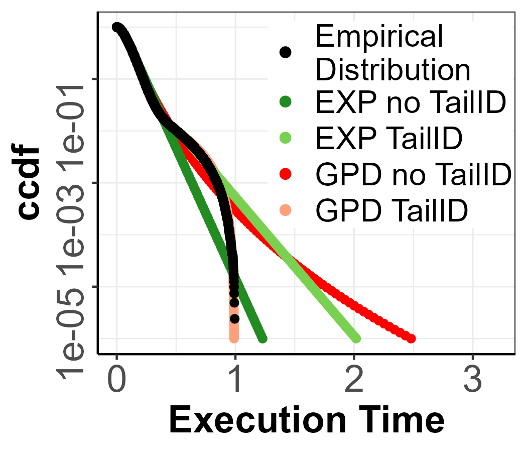
We illustrate with a parametric distribution example how even when the IID hypothesis on the whole distribution and the tail (see Remarks 7 and 8) have not been rejected, the WCET estimation can be misleading as it does not account for low-density mixtures in the tail. In particular, we generate a Gaussian mixture model, with one component having of the weight with mean and standard deviation and the second component having weight , mean and standard deviation . The use of a Gaussian distribution is useful as an example because it has exponential tails, so even in the presence of mixtures, theoretically the tail is localized in the second component with an EVI .
The parametric distribution data, which can be seen in Figure 1(a), was used to compute the pWCET estimate considering two models: a GPD model that can take either light or heavy tails, and an exponential model (recall that the exponential model is the theoretically appropriate one given the Gaussian distribution). The estimation of the threshold, , is performed throughout the paper with a threshold selection algorithm based on QQ plots [6], although other methodologies can be used to obtain similar results [42]. In Figure 1(b), we show the extremogram for the parametric distribution. The quantile chosen for the extremogram, the quantile, is based on the original work [18], and also employed in [41]. Furthermore, the cutoff value for the extremogram, to determine if there is no dependency, is set at following [41]. Figure 1(b) shows a value for the extremogram lower than , which indicated no dependency among extreme values.
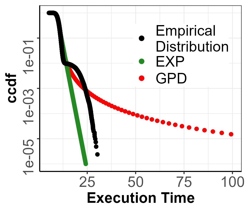
The pWCET estimates are shown in Figure 1(c). Note that, the black points represent the CCDF of the observed values in Figure 1(a). In the case of the GPD, it produces heavy tails, given that EVI is bigger than . This is due to the threshold selection detecting that the tail begins before the second component of the mixture, which produces a seemingly heavy tail because the rest of the extreme points are further apart. This results in pessimistic upper-bounds, more than 3 times bigger than the actual tail for low probabilities. In the case of the EXP, the threshold has been selected before the second component, and thus the pWCET estimate is optimistic. Overall, this example highlights the connection between a miscalculation of the threshold due to mixture distributions and misestimation of the EVI and the subsequent impact on the pWCET estimation.
4 Uncertainty Analysis for the GPD
Most EVT methods to estimate the tail build around the stability of the EVI from a certain threshold onward [25, 15]. However, in the presence of low-density mixtures in the tail, the EVI can be found to be unstable for higher thresholds due to low amount of information, and therefore miscalculated. We showed in Section 3 how this misestimation can compromise the pWCET estimations given the threshold selected are lower due to the presence of low-density mixtures. In order to detect low-density mixtures in the tail and avoid such scenarios, this section develops on the principles of the estimation of the EVI and how the estimations can change as we approach low-density mixtures in the tail. In fact, detecting and quantifying this change in a robust manner is the goal of this work and the core principle of TailID.
4.1 Maximum Likelihood Estimation and Uncertainty Analysis
Given observations from a random variable , and considering the excess random variable over a threshold , defined as in Equation 1, the parameter of the GPD can be estimated. Apart from the model uncertainty associated to the expression, the estimation of will also contain sampling uncertainty due to the variability of the input, . To assess the uncertainty around the estimated EVI, , of the GPD, it is necessary to compute a confidence interval, which gives a range of values within which the true parameter is likely to lie with a specified level of confidence .
The classical method of calculating the confidence intervals for an estimator is to derive the asymptotic distribution of the errors. That is, the difference between the true value of the parameter and the estimator has a distribution which can be found. If the estimator is drawn from Maximum Likelihood Estimator (MLE) method, said difference converges in distribution to Gaussian as:
Theorem 9 (Asymptotic Normality of the Estimator [49]).
Let be the parameter’s true value and the Maximum Likelihood Estimation of , and the sample size, then:
| (4) |
the difference between the true value and the parameter’s estimations converges in distribution to a Gaussian distribution .
This theorem combines key probabilistic results, specifically the Law of Large Numbers and the Central Limit Theorem. Equation 4 is a classical result found in many foundational probability and statistics books [49] [32]. In order to unfold Equation 4 we need to find the MLE of the Extreme Value Index, , and its variance, . Then, Equation 4 allows us to compute confidence intervals on the estimation of .
First, we introduce the Maximum Likelihood Estimation (MLE) [35] method for parameter estimation, as it is the approach utilized in Equation 4. One of the most common methods for estimating the parameters of a distribution, in particular the EVI, , of the GPD, is MLE [35]. MLE is a statistical technique employed to find the parameter’s value that maximize the likelihood function, given a set of observed data. The likelihood function for a sample from a distribution with parameter is given by:
Definition 10 (Likelihood).
Let the sample of a random variable of size with probability density function , then the likelihood function is defined as
| (5) |
where is the probability density function (PDF) of the distribution at given parameter .
Now, the log-likelihood is defined as:
Definition 11 (Log-likelihood).
Let be the PDF at given parameter , then
| (6) |
is the log-likelihood function given parameter .
The MLE for , denoted , is the value that satisfies the following equation:
Definition 12 (Maximum Likelihood Estimation).
Given a log-likelihood function , is the value of the parameter which maximizes the log-likelihood, that is:
| (7) |
We now have the tools to prove the MLE of the EVI of the GPD.
4.2 Computing Confidence Intervals on the Extreme Value Index
Now we employ the definitions above for the particular case of the GPD. In the case of the GPD, given observations and considering the excesses for a given threshold , , the likelihood function of the GPD is:
| (8) |
then the log-likelihood function takes the form:
| (9) |
Taking the change of variables ,
| (10) |
Performing MLE to obtain :
| (11) |
This leads to:
| (12) |
Given that the Extreme Value Index, , cannot be totally isolated, this expression needs to be solved numerically. To achieve this, the gpd.fit() function from the ismev package [21] is used to fit a GPD model to threshold exceedances using MLE.
In order to compute the variance of a parameter , , we can use the Cramér-Rao bound, which finds the estimator with the lowest variance based on observations of a random variable , thus reducing the uncertainty [39]. The Cramér-Rao bound is stated as:
Theorem 13 (Cramér-Rao bound).
Let be a parameter with an unbiased estimator , then the variance of the estimator is bounded by
| (13) |
where is the Fisher information.
The Fisher information is defined as:
Definition 14 (Fisher Information).
Let a likelihood function given a parameter , then
| (14) |
which uses the expected value of the derivative of the MLE estimator. With this mathematical framework, we can compute the uncertainty around the MLE of the Extreme Value Index that we introduced in Equation 4.
Following the procedure indicated in Equation 13, the Cramér-Rao bound for the EVI is
| (15) |
Then, the Fisher information, for known, is computed as:
| (16) |
Plugging this result into Equation 13:
| (17) |
Finally, we complete Equation 4 for the case of the GPD
| (18) |
Equation 18 allows us to compute confidence intervals for the estimation of the EVI.
Example 15.
Let us consider a set of observations with an estimated parameter using Equation 12. We want to compute the confidence interval for at a confidence level of . According to Equation 18, we have:
| (19) |
To construct a confidence interval, we define and recall that satisfies:
| (20) |
where represents the -quantile of the standard normal distribution. For , .
Using the standardization from Equation 19, we obtain:
| (21) |
Rearranging the inequality, we get:
| (22) |
Consequently, the confidence interval for is given by:
| (23) |
recalling that and .
Given that we are using the MLE, we are reducing the model uncertainty as much as possible, while being able to capture the variability of the estimator.
Finally, the expression in Equation 18 is the core of the TailID algorithm, as it will be used to assess whether a change in the tail is present.
5 TailID methodology
The proposed approach, TailID, relies on the fact that low-density mixtures in the tail causing changes in the tail behaviour manifests in a change of the EVI . TailID builds on the theoretical development we showed in Section 4. In particular, the core of the algorithm is the confidence intervals of the MLE of the EVI of the GPD in Equation 18.
TailID algorithm analyzes iteratively the extreme values that may be triggering a change in the EVI , one by one, until a change of tail behaviour is detected or all points are processed. Note that, an estimation of that falls outside the confidence intervals, does not imply that the estimation is inappropriate, but that the behaviour has changed due to the detected mixture component and therefore we should apply a more nuanced tail analysis by taking into account the presence of mixtures in the tail estimation.
TailID, detailed in Algorithm 1, works on a sample data , a confidence interval , an extreme value percentile , a percentile for the candidate points , and returns the set of points that are more sensitive to the hypothesis of the sample data being ID. Sensitive points are those that, if considered in the sample, can cause the EVI to fall outside the confidence interval computed without them. Also, TailID is agnostic on the number of compounded distributions in the mixture as it considers the last component (before the point breaking the ID assumption) for tail estimation by selecting a sufficiently high percentile of points . In Section 5.1, we show how we set to detect the last component.
The algorithm first initializes the data structure (line 2) where sensitive points are stored. Given a time series , the implemented algorithm applies the PoT method to select the tail of the distribution. The threshold for the PoT is computed based on the extreme value percentile such that percent of the data in falls below , i.e., Quantile (line 3). In this work, the threshold selection algorithm is drawn from [6]. From the definition above of , the excess of the time series is defined as
Next, we determine an initial ordered set of candidate points that are considered as the most sensitive to the assumption of the sample being ID. The definition of depends on the input parameter that is used as the criteria to define the first candidate as
| (24) |
where, . Both choices of and will be discussed in Subsection 5.1. The ordered set of candidates is therefore initialized (line 4) as
| (25) |
For each of the candidates in , the algorithm will check whether it has a significant impact on the ID hypothesis. For this purpose, it is necessary to consider the set with the elements in removed, that is (line 5). The excess sample is then computed on (line 6) as
| (26) |
The subset is then used (line 7) to estimate the reference EVI parameter of the sample, denoted by . This step is crucial for understanding the core principle of TailID. The values in are the tail of the distribution with part of the most extreme values removed and collected in the set for later use.
As the last step in the initialization phase (line 8) the TailID computes the confidence interval for this EVI, , at confidence level . TailID estimates the range within which the true parameter value of the distribution of the maximum extremes is expected to lie with a probability of , characterizing the tail behavior. The argument is, that if there are no mixtures in the tail, the re-estimation of the EVI adding back the stored extreme values in , will still fall within the confidence interval. The confidence interval is recomputed at each iteration of the core block of the algorithm to account for the additional information contributed by each extreme value in that is not added to . The implications in the choice of and the suggested value will be discussed in Subsection 5.1.
The core of the algorithm applies to each element (line 9) which is added back to the sample as , line 11. As is an ordered set, the first candidate value will be the closest value to the sample mean, being the first point of the ordered set . Subsequently, the excess will be computed on the new extended sample set (line 12), again according to Equation 26.
The new computed excess set is then used to fit the EVI (line 13). Now if does not fall inside the confidence interval (line 14),
| (27) |
there is sufficient evidence to conclude that is sensitive to the hypothesis of the tail of the time series being ID. So it will be added to the set of ID-Sensitive Points (line 15). Instead, if falls inside the confidence interval , then it will not be added to and will be used to update the confidence interval for the next candidate value (line 17).
The algorithm iteratively analyzes all elements in , following the same procedure until the first ID-Sensitive Point among the candidates is found. At that point, since is an ordered set, also all the following candidates, , are sensitive and will be added to (line 20). This latter behavior is enforced under the assumption of being empty until the first sensitive point is found (line 10).
Finally, the algorithm returns as the list of sensitive points breaking the ID assumption (line 23).
From a theoretical perspective, it is worth considering that TailID builds on a ordinary set of assumptions. First, it assumes that the tail of the data follows a GPD. Second, the validity of the confidence intervals in Equation 18 requires the asymptotic normality of the MLE of the EVI . This, in turn, depends on regularity conditions. Specifically, the data are assumed to be IID with PDF such that for , the parameter space is compact, and the true parameter lies in its interior. Moreover, is continuous in with probability one, and . In addition, the function is assumed to be twice continuously differentiable and strictly positive in a neighborhood of . The following integrability conditions must also be satisfied: , and . Furthermore, the Fisher information matrix must exist and be nonsingular, and it is required that [36].
5.1 Discussion of Algorithm Parameters
Algorithm 1 works on three main parameters (, , and ) that call for a careful selection to guarantee the effectiveness of the results. In the following we discuss the implications on the parameter selection and the proposed selection criteria.
. The choice of parameter determines the points in the sample that are considered part of the sample tail. Given the lack of consensus in the literature regarding the choice of percentile that defines the sample tail, several studies also criticize the practice of arbitrarily selecting a fixed percentile without first analyzing the data [43]. To address this, we determine using the methodology developed in [6] that evaluates multiple candidate percentiles and selects the one that best aligns with the assumptions of EVT. Any other threshold selection algorithm in the literature is also suitable.
. The choice of determines the points in the sample that are considered candidates for being sensitive points. This percentile is tied to the selection of , such that, the candidates for sensitive points must belong to the sample tail and indeed represent data with very low probability outcomes. Additionally, as the goal of the TailID algorithm is to detect any inconsistencies in the ID of the tail, we avoid selecting a percentile that fails to detect any sensitive points while another percentile does. A Grid Search algorithm [9] employed on the kernel data, described in Section 6, has shown that choosing results in a stable number of detected sensitive points across different values of , and across multiple scenarios. Moreover, this percentile ensures that the algorithm consistently identifies a relevant proportion of sensitive points among the candidate points, e.g. for typical thresholds between percentiles , the candidate points selected are the top and of the sample respectively. Thus, we are aiming at the last component in the mixture. This choice minimizes the risk of failing to detect sensitive points when compared to other percentiles. Also, to improve robustness, we perform a grid search on the data before applying the algorithm. This preliminary step helps to determine an appropriate percentile .
. The confidence level is set at to identify only those points that truly impact the tail distribution, thereby minimizing the number of false positives. For a point to be classified as sensitive, the EVI of the tail, recalculated to include this point, must fall outside the confidence interval of the EVI computed without it. With , the risk that the true parameter of the distribution lies outside this range is .
5.2 Decision Making on TailID outcomes
TailID improves the interpretability of the outcomes, allowing the user to extract conclusions on the extreme values of the data at analysis. In this line, we next define several outcomes (scenarios) from the execution TailID and how to interpret them. In order to create these scenarios we consider the minimum amount of samples (MoS) required for a proper estimation of the EVI. The topic of determining the necessary amount of extreme samples to obtain an accurate estimation on the tail is outside the scope of this work. However, we refer to works in other areas where they argue that the minimum number of extreme samples varies depending on the tail profile [34, 28]. The authors in [14] develop a method to estimate the MoS for each sample where, in general, it ranges between and . In line with it, in this work we conservatively set MoS to be at least and rely on [14] for further tuning. For instance, for an Extreme Value Index and , the confidence interval is .
Overall, using the number of inconsistent points detected, that is the cardinality of the set (i.e., ), we define three scenarios according to how compares to :
Scenario 1.
() No inconsistent points detected. If the list of inconsistent points, , is empty, then no candidate point fell outside the confidence intervals, and the ID hypothesis on the identical distribution of the tail holds. The TailID outcome provides more evidence on the robustness of the tail estimations given the stability of the tail. In this scenario, TailID in conjunction with the KPSS test for the stationarity on the whole distribution, provides a solid analysis on the sample
Scenario 2.
() High-number of inconsistent points detected. If the final list of inconsistent points detected by the TailID algorithm is bigger than theMoS required for a proper estimation of the EVI, then we are in the presence of multiple tail behaviors, which should be taken into account when performing pWCET estimations. Hence, the sample needs to be analyzed taking into account the presence of another source of uncertainty in the tail of the distribution. In this scenario, TailID considers the threshold of the tail at the first inconsistent value found with TailID, which would be on the last mixture component. Interestingly, in the case of multiple mixture components conforming the distribution, the PoT model implies that the last component would be employed for the tail estimation, while the rest would be considered on the bulk of the distribution.
Scenario 3.
() Few inconsistent points detected. As in Scenario 2 there is mixture, but in this case more samples are needed to make a better estimation of the parameters of the distribution since with less than MoS points it would be imprecise. If after performing more runs , we apply TailID as in Scenario 2. However, if the user reaches the number of runs he/she can perform – e.g. due to the associated time required to perform the runs – and still , tail prediction should not be done otherwise the uncertainty in the estimation can be high.
6 Experimental Evaluation
We make a two-fold evaluation of our proposal. On the one hand, we build on a set of parameterized mixture distributions that allow us to ascertain how our technique works for scenarios of different complexity. Since we know the actual distribution of the tail, we can assess and assure with complete certainty the accuracy of TailID for the evaluated scenarios. On the other hand, we assess TailID on execution time samples collected on a state-of-the art board for embedded automotive systems, the NVIDIA AGX Orin.
6.1 Parametric Distributions
We use Weibull, Beta and Exponential distributions as they have different types of tails [4, 47]: the Weibull has a sharper slope and a maximum value; the Gumbel (Exponential tail) also has a relatively sharp slope but it has no maximum; and the Beta (light tail) distribution has a similar profile to the Weibull and is frequently used to model high quantiles of random variables with a finite specified interval, hence suiting WCET modeling.
From these uni-modal distributions we build the parameterized mixtures shown in Table 3, which specifies the parameters and weights of both components, the theoretical EVI. The goal when building the parametric mixture distributions is to ensure variety in three main aspects: i) the tail profile, ii) the sharpness of the tail, and iii) the density of the last component. For the tail profile, we select three different parametric distributions in Weibull, Beta and Exponential. For the sharpness, we select a different shape parameter for the distributions (the shape for Exponential is the same given that the EVI is always 0). Finally, we select a different density of the last component by changing the weight of each parametric distribution. With these three aspects, we are able to cover a wide variety of cases that are representative of WCET analysis scenarios.
| Acronym | Type | Parameters | EVI | EVI | EVI | |
| TailID | noTailID | |||||
| MixW_1 | Weibull |
|
||||
| MixW_2 | Weibull |
|
||||
| MixB_1 | Beta |
|
||||
| MixB_2 | Beta |
|
||||
| MixE_1 | Expntl. |
|
MixW_1.
Figure 2(a) shows the sample where points targeted as candidates by the algorithm are marked with distinct shapes and colors, differentiating them from the rest. The red-shaded area highlights the points ultimately detected as inconsistent by the algorithm.
In Figure 2(b), the horizontal gray line represents the GPD EVI of the sample’s extreme set without including the candidate points, while the dashed line indicates the upper bound of its confidence interval. Each point corresponds to the GPD EVI when the candidate point (represented with the same color in the Figure 2(a)) is added to the sample’s extreme set, with each dashed line representing the upper bound of the confidence interval for that configuration. For instance, in Figure 2(b) the first candidate, the purple solid circle, is below the grey dashed line, therefore within confidence intervals. Then the confidence interval is recomputed considering the first candidate, and is shown in a dashed purple line, just above the grey dashed line. TailID iterates this process until the yellow square is found to be above the confidence interval, therefore inconsistent with the ID hypothesis. Finally, the yellow square can be used as the new threshold from where to estimate the pWCET.
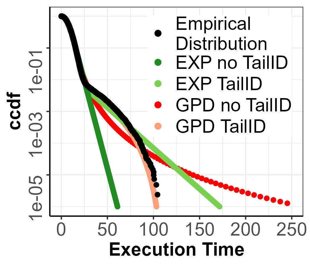
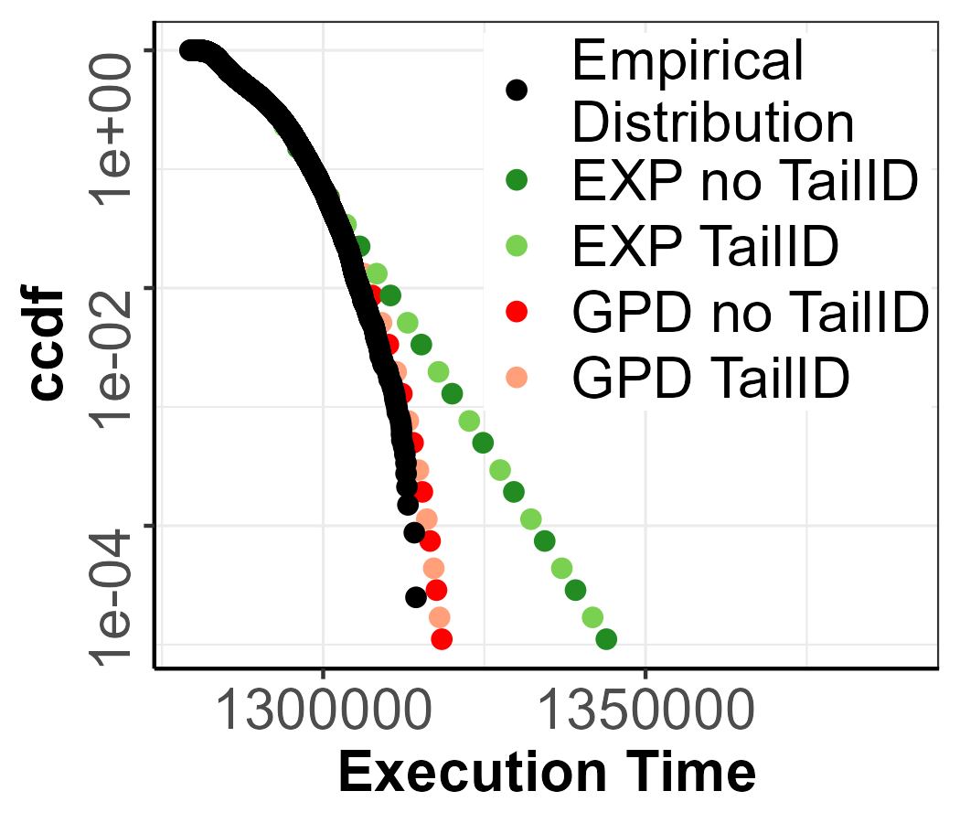
The pWCET estimates with GPD and exponential tail (EXP) fitting are shown in Figure 2(c). In particular, we use the sample in Figure 2(a), which has size , to estimate the exceedance probability We distinguish two scenarios: no TailID in which pWCET estimates are obtained with the first threshold selected taking the sample as is (dark green and blue projections); and the TailID in which pWCET estimates are obtained with TailID, i.e. using the new threshold found represented by the yellow square (light green and blue projections). The black dots represent the reference CDF of MixW_1 up to probability which is used as ground truth.
For the no TailID scenario, the EXP model, which is usually deemed as trustworthy, produces an optimistic bound, while the GPD model produces a pessimistic bound. In the TailID scenario produced estimates with GPD and EXP are tighter: GPD results in a tighter tail yet slightly underestimating, while the EXP model produces the expected trustworthy pWCET with a tight estimation. The actual estimated EVI parameters for each model and scenario can be found in Table 3, where we can see that in all cases the EVI in no TailID produces heavy-tails, while the TailID scenario produces an EVI which is close to the real one reflected in the EVI column, which is the exact value for each distribution. The EVI for the EXP models is always exactly 0.
Overall, TailID brings a clearly positive impact on pWCET estimations. For the GPD models, the pessimism is reduced while occasionally incurring negligible underestimation when compared to that incurred by the EXP model in no TailID. Additionally, for the EXP models, TailID significantly reduces underestimation.
Rest of the distributions.
Figure 3 shows the candidates and inconsistent points detected for the rest of the parametric distributions in Table 3. There we show how for each distribution, the number of inconsistent points detected is different, with 52 for MixW_2, 24 for MixB_1, 28 for MixB_2 and 92 for MixE_1.
As we can see in Figure 4, the inconsistent points detected for all distributions are always found in the domain of the last mixture component, which can also be seen in Figure 3 where the red-shaded area is always found separately from the bulk of the distribution and it is different for each parametric distribution. For instance, in Figure 3(b), the first candidate points are not far from the bulk of the distribution, and therefore they could be considered as extreme values from the first component. Figure 4(b) confirms that suspicion, given that the first candidates are within confidence intervals, therefore, not belonging to the last mixture component. However, this assumption is broken at the magenta triangle point, which is much further from the bulk of the distribution, as seen in Figure 3(b) where the last mixture component has been detected. A similar scenario is captured in Figure 2(b) and 4(c). In Figures 4(a) and 4(d), we observe how the first candidates are already detected as inconsistent and, from Figures 3(a) and 3(d), it is not obvious that a mixture is present.
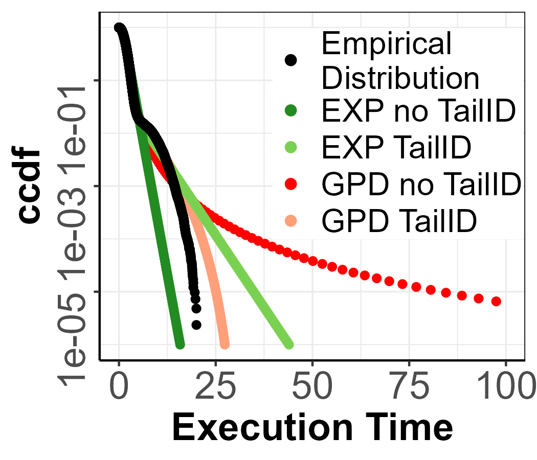
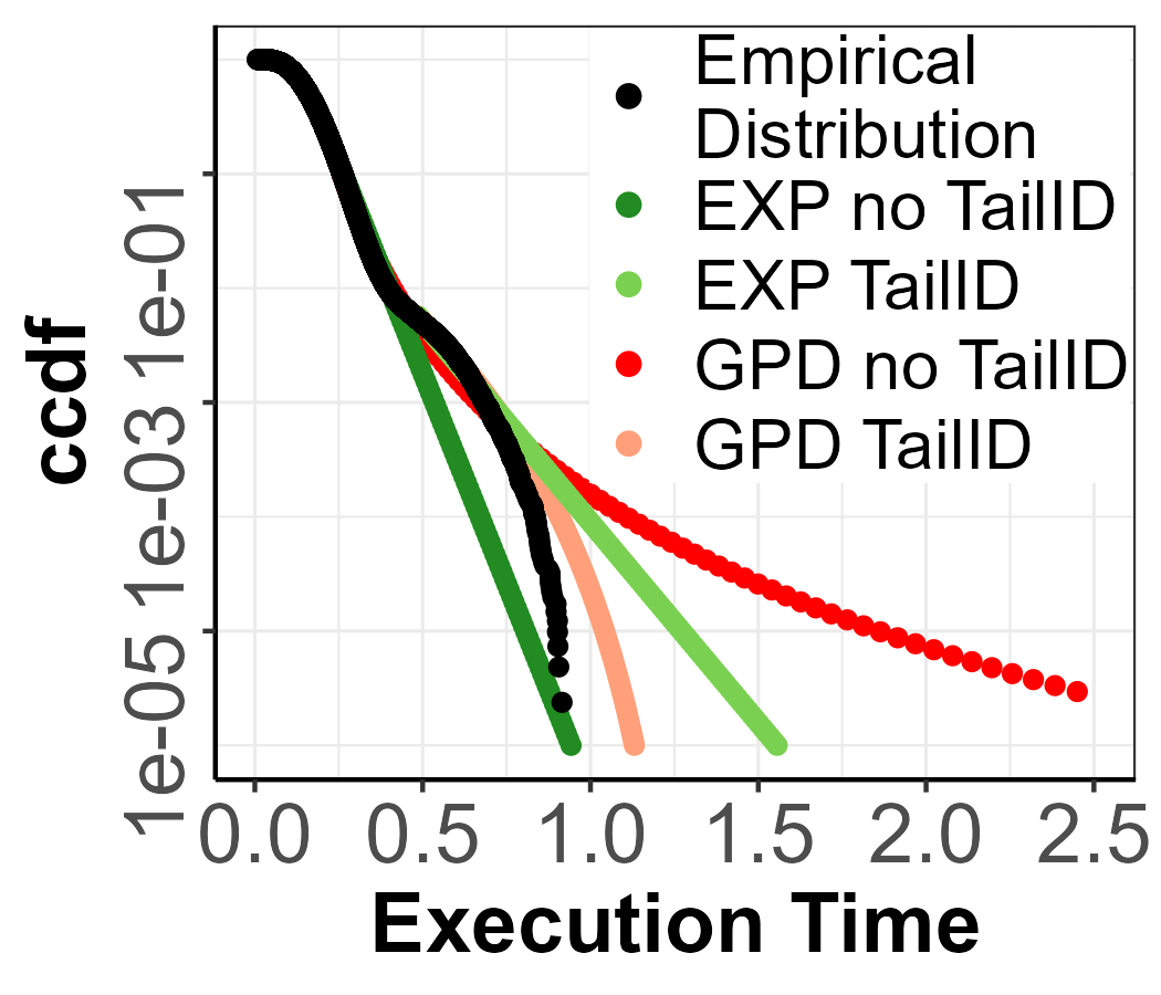
All of these findings are reflected in Figure 5 where the pWCET estimations for the rest of the parametric distributions are found. In more detail, the GPD with no TailID always produces a heavy tail, thus leading to a pessimistic bound (dark blue line). With TailID, the GPD model produces tighter bounds (light blue). For the EXP model, which is regarded as a trustworthy upper-bound, with no TailID there is risk of computing optimistic bounds as the threshold estimated is too low (dark green line). Instead, with TailID the EXP model consistently produces tight upper-bounds (light green line), given that the chosen threshold using TailID is on the last mixture component.
6.2 NVIDIA Orin AGX
Setup.
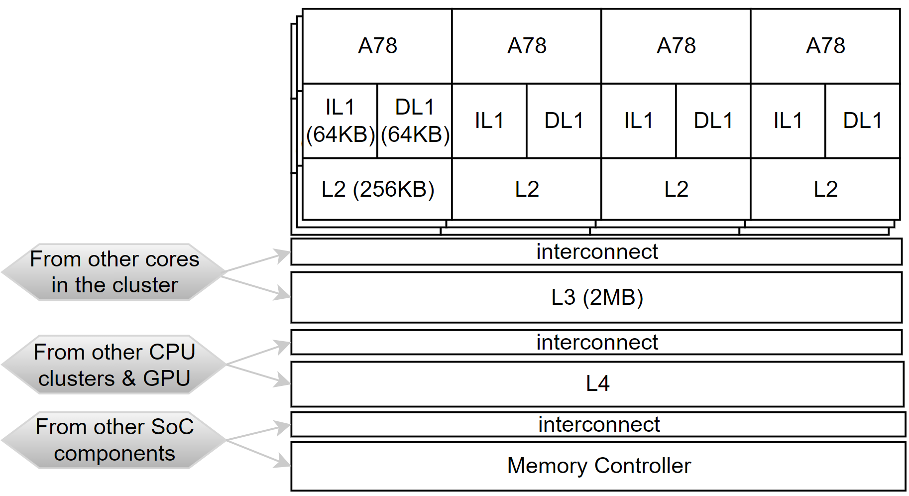
In this work we cover the execution time variability from the hardware and system software. At the application software level, we build on representative kernels that in general present low execution time variability. In particular, we focus on the three A78 clusters of the Jetson 64GB AGX Orin, simply referred in this work as Orin, a representative high-end MPSoC for the automotive domain [27]. An Orin CPU cluster implements four high-performance Arm® Cortex®-A78AE v8.2 cores each with its private data and instruction caches (iL1 and dL1, respectively in Figure 6) and a unified private L2 (L2). An L3 cache is shared at the cluster level. The L4 is mainly shared between the CPU and the GPU, with misses going to a system-level fabric and the memory controller. We use the default Linux-based setup provided by the manufacturer to run our experiments.
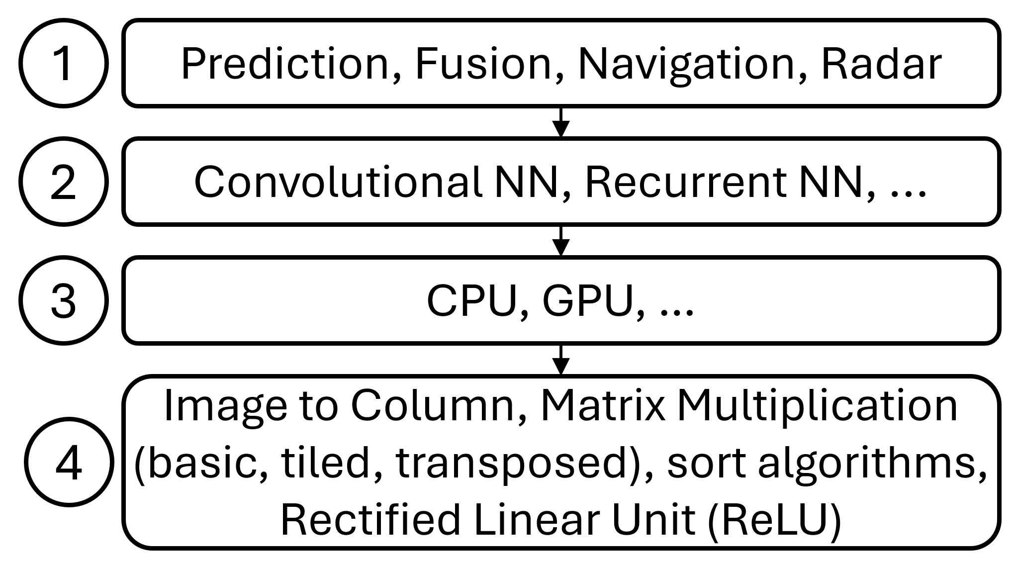
At the application level, we tested the performance of the TailID for several kernels used in AI-based edge applications, see Figure 7. At the top level applications \small{1}⃝ like autonomous driving and radar applications [22, 46], object detection, data fusion, and navigation are AI-fuelled and build on different types of Neural Networks (NN) \small{2}⃝ like recurrent and convolutional. As MPSoCs like the Orin allow consolidating several applications, there can be multiple NNs instances running on the CPU and accelerators \small{3}⃝. CPU is used when accelerators are busy or the working set is reduced and the overheads to offload the kernels (along with its data) to the accelerator is too high [44].
Applications build on AI libraries that include as a central operator (function) matrix multiplication [45], which accounts for a large portion of the execution time (beyond 65%) [20]). image-to-columns is used in convolutional for tensor lowering to enable matrix convolutions. Another common operator is rectifier that is the positive value of its argument [5]. Other pervasive functions in those libraries is vector-dot-product and matrix transpose [45]. Overall we use the kernels MM basic and tiled, Image to Column, sorting algorithm, Matrix transpose, and Rectified Linear Unit.
Results.
With these kernels we build randomly generated workloads from 2 to 12 kernels each. From the execution times for each workload, we perform an initial filtering step. Specifically, we apply three statistical tests (KPSS for stationarity, BDS for short-range dependence, and the Hurst index for long-range dependence) following the methodology of Reghenzani et al. with the PPI test [40]. Additionally, we use the extremogram test to assess dependence in the extremes and apply the KPSS test to the tail as an initial approach for identifying identical distribution in extreme values. This analysis follows Remarks 7 and 8.
Out of the initial initial workloads, cases were not rejected in any test and kept them for further analysis, the remainder does not meet the conditions for the application of EVT. As mentioned in Section 2, the PPI test is an already strict test that sets a high bar for the trustworthy application of EVT. We then apply TailID to the workloads which pass the IID test. From these cases, also passed the ID hypothesis for the tail, as no inconsistent points were detected (scenario 1). On the other hand, workloads resulted in with less than MoS IPD (scenario 3). Finally, for workloads the TailID algorithm detected more than MoS IPD. Therefore, TailID was able to automatically detect several workloads that do not fulfill the ID hypothesis in the tail. Next, we illustrate some workloads filling in the different scenarios.
inconsistent points.
parameter.
applying TailID.
inconsistent points.
parameter.
applying TailID.
inconsistent points.
parameter.
inconsistent points.
parameter.
and inconsistent points.
and inconsistent points.
Scenario 1.
Figure 8 presents an example workload in which TailID confirms that the execution time series satisfies both the ID hypothesis for the tail and the and the combination of the three tests (KPSS test, BDS test, and Hurst Index) as discussed in [40]. In Figure 8(b) we can see how all the EVI estimations fall under each confidence interval, therefore providing the evidence that the tail is ID. Figures 8(c) show the pWCET estimations in the no TailID and TailID scenarios in a similar fashion to the parametric distributions in Section 6.1. In this case, we employ a sample of size to estimate the pWCET in both scenarios for the exceedance probability . Note that in Figure 8(c), the pWCET for the no TailID and TailID scenario is the same, given no inconsistent points were found.
Scenario 2.
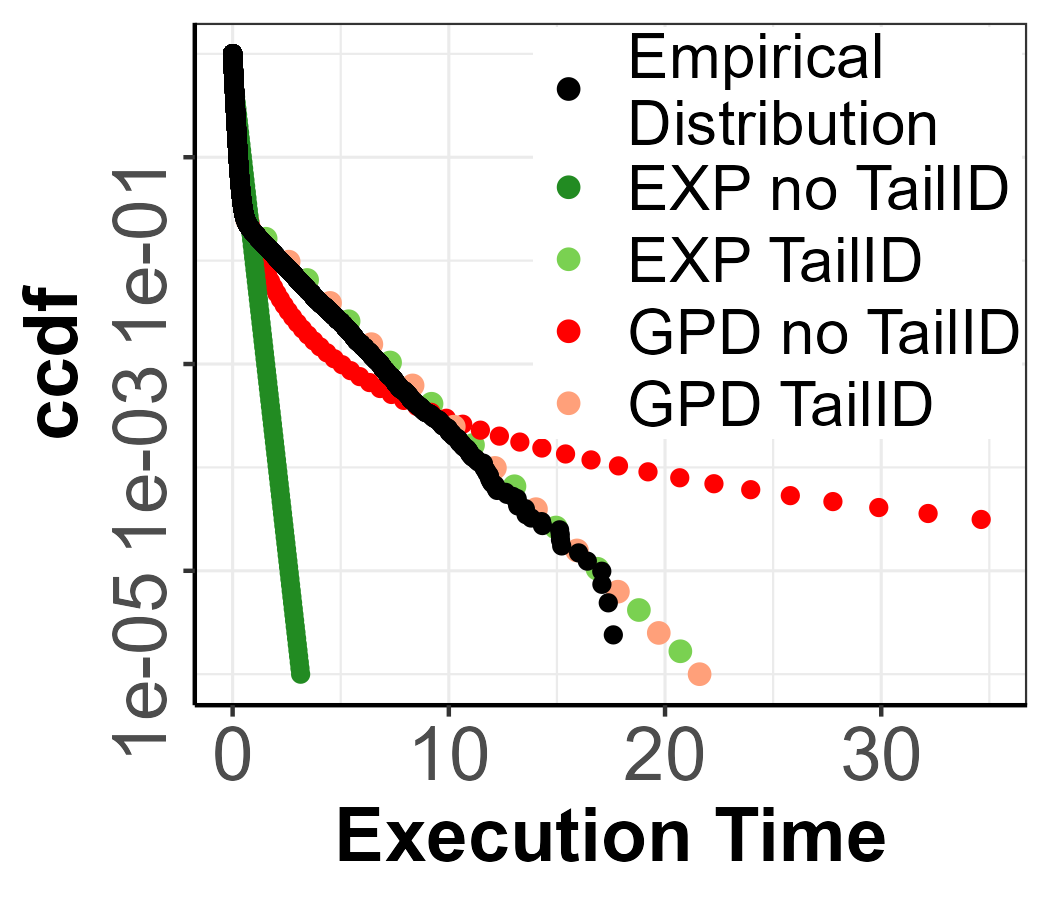
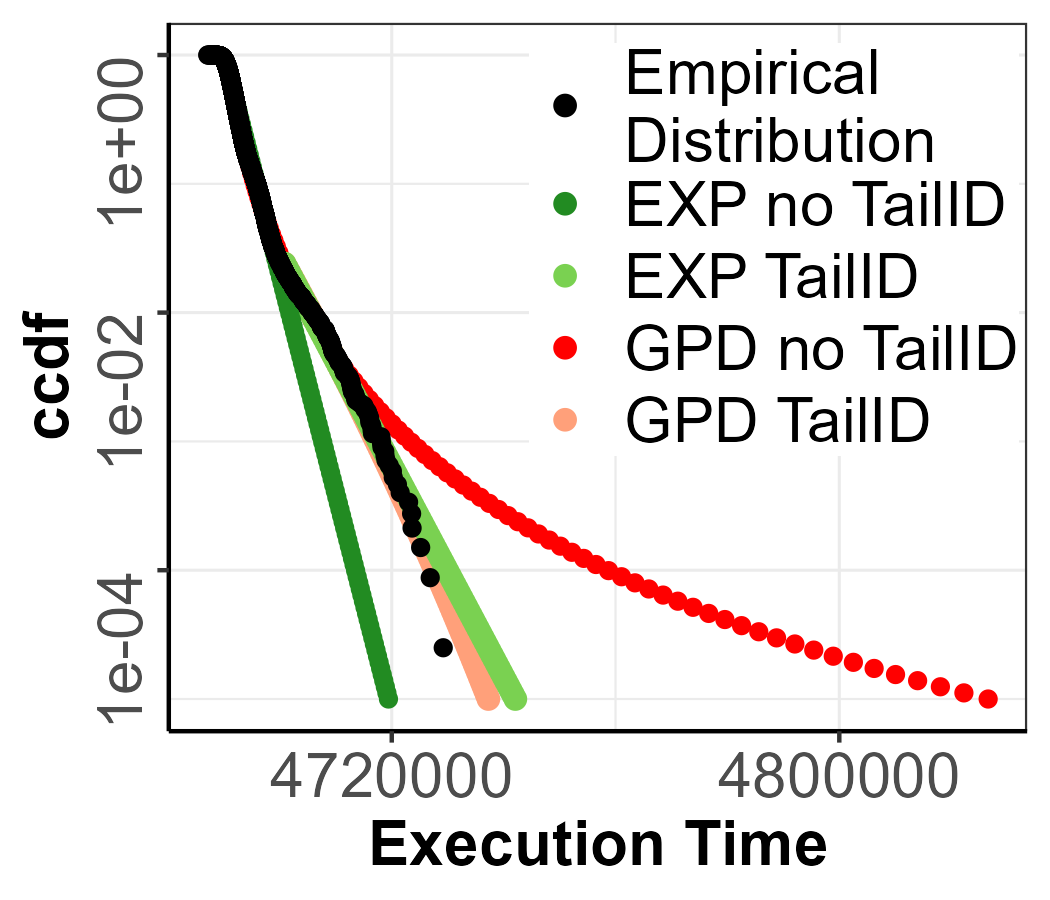
In this case, the combination of the three tests (KPSS test, BDS test, and Hurst Index)[40] does not reject the non-stationary of the execution time series, but TailID detects more than 40 inconsistent points. In Figure 9(a) we can see how the extreme values are spread out and not far from the bulk of the distribution, which can easily confuse the threshold selection. However, TailID is able to find inconsistent points in the first candidate points similar to the parametric MixW_2 and MixE_1 scenario. The pWCET estimates, see Figure 9(c), confirm that detecting a low-density mixture in the tail and, hence, choosing the appropriate threshold, produces a tighter upper-bound with the GPD and EXP models. A quantitative assessment of the improvement achieved with TailID can be performed for each specific quantile level , at which the pWCET is evaluted, considering the defintion of pWCET tightness as For example, at , the GPD model yields a tightness of 1.0068 without mixture detection and 1.0004 with TailID. For the EXP model, tightness goes from 0.9973 to 1.0008 when TailID is applied.
Scenario 3.
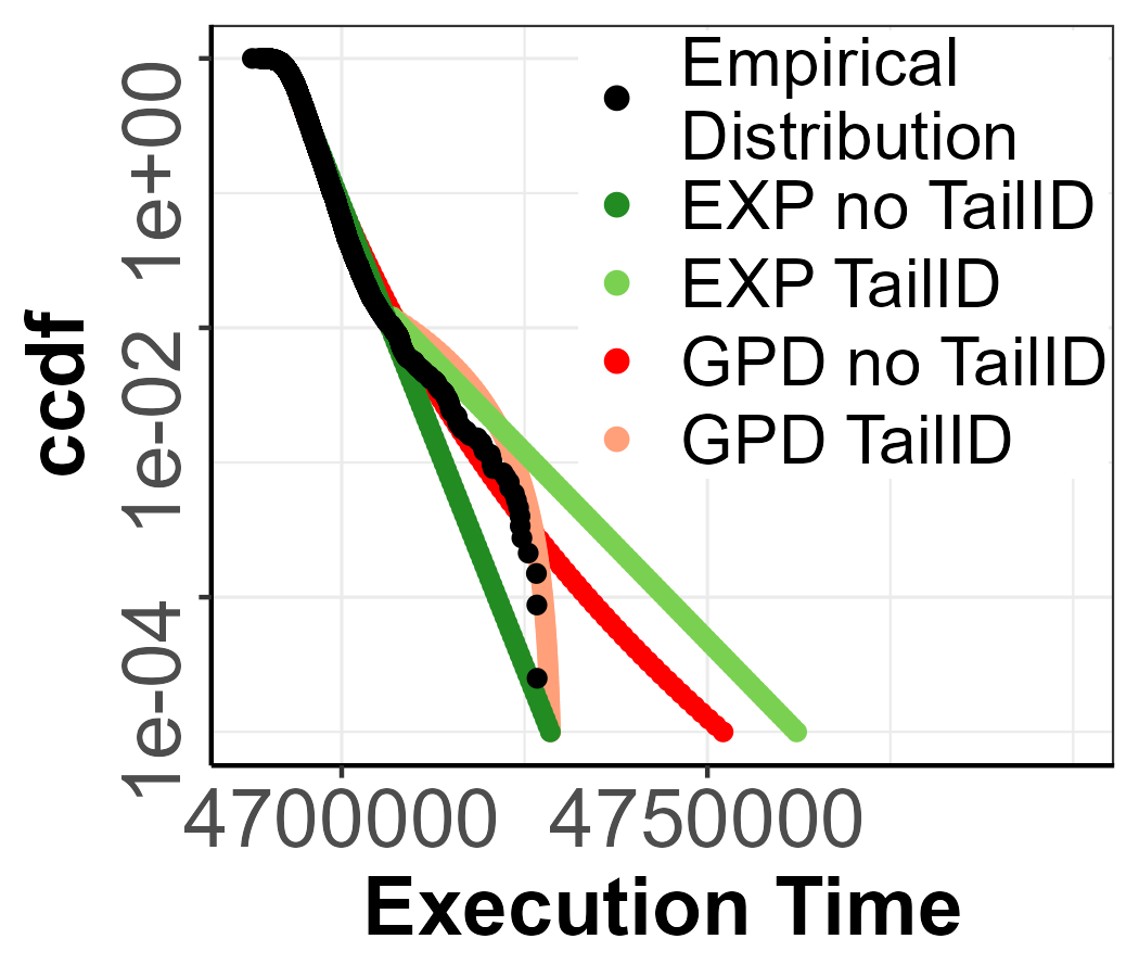
In this case, the KPSS test, BDS test, and Hurst Index [40] do not reject IID of the execution time series and TailID detects few inconsistent points within the selected candidates, so more runs are required. We illustrate the two possible outcomes (sub-scenarios) identified in Section 5. First, in Figure 10(a,b) TailID detected , and after performing more runs we see the impact in 10(c,d) where . And second, in Figure 11, instead, even after performing more runs and reaching the maximum number of runs, still holds. In both sub-scenarios, Figures 10(b,d) and 11(b,d), we can see that the TailID selects the inconsistent point when the evolution of the GPD EVI changes, which indicates a change in tail distribution. For the first sub-scenario, Figure 10(e) shows how TaiID make EXP and GPD estimates much more accurate.
7 Conclusions
The execution of increasingly rich software functionalities on top of cutting-edge MPSoCs can result in low-density mixture execution time distributions. As discussed in Section 3, the presence of low-density mixture distributions in the tail of the data challenges the trustworthiness of timing bounds computed by EVT-based approaches. Traditional tests for identical distribution, typically applied on the full data and not on the tail, are anyway unable to detect low-density mixtures. We leverage key principles in EVT methodology and propose TailID an algorithm building on extreme value index confidence interval for testing the ID hypothesis specific on the tail of the data, and elaborate a practical strategy to follow for enabling EVT trustworthy application under all possible test outcome. We assessed our approach on both parametric distributions and real execution data collected on a reference MPSoC in the embedded domains, confirming that TailID is able to detect low-density mixture in the tail on data sample, even in those sample that already passed state-of-the-art IID tests. For this reason, we contend TailID has to be used in conjunction with state-of-the-art IID tests to guarantee a more robust data analysis framework for increases confidence in EVT estimations.
References
- [1] Jaume Abella, Carles Hernandez, Eduardo Quiñones, Francisco J. Cazorla, Philippa Ryan Conmy, Mikel Azkarate-askasua, Jon Perez, Enrico Mezzetti, and Tullio Vardanega. Wcet analysis methods: Pitfalls and challenges on their trustworthiness. In 10th IEEE International Symposium on Industrial Embedded Systems (SIES), pages 1–10, 2015. doi:10.1109/SIES.2015.7185039.
- [2] Jaume Abella, Maria Padilla, Joan Del Castillo, and Francisco J. Cazorla. Measurement-based worst-case execution time estimation using the coefficient of variation. ACM Trans. Des. Autom. Electron. Syst., 22(4), June 2017. doi:10.1145/3065924.
- [3] Tadeu Nogueira C. Andrade, George Lima, and Verônica Maria Cadena Lima. Drawing lines for measurement-based probabilistic timing analysis. In 2024 IEEE Real-Time Systems Symposium (RTSS), pages 243–255, 2024. doi:10.1109/RTSS62706.2024.00029.
- [4] Charalampos Antoniadis, Dimitrios Garyfallou, Nestor Evmorfopoulos, and Georgios Stamoulis. Evt-based worst case delay estimation under process variation. In 2018 Design, Automation & Test in Europe Conference & Exhibition (DATE), pages 1333–1338, 2018. doi:10.23919/DATE.2018.8342220.
- [5] ApolloAuto. Perception, 2018. URL: https://github.com/ApolloAuto/apollo/blob/r3.0.0/docs/specs/perception_apollo_3.0.md.
- [6] Luís Fernando Arcaro, Karila Palma Silva, and Rômulo Silva De Oliveira. On the reliability and tightness of gp and exponential models for probabilistic wcet estimation. ACM Trans. Des. Autom. Electron. Syst., 23(3), March 2018. doi:10.1145/3185154.
- [7] August Aimé Balkema and Laurens de Haan. Residual Life Time at Great Age. The Annals of Probability, 2(5):792–804, 1974. doi:10.1214/aop/1176996548.
- [8] K. Berezovskyi, L. Santinelli, K. Bletsas, and E. Tovar. Wcet measurement-based and extreme value theory characterisation of cuda kernels. In Proceedings of the International Conference on Real-Time Networks and Systems (RTNS), pages 279–288, 2014. doi:10.1145/2659787.2659827.
- [9] James Bergstra, Rémi Bardenet, Yoshua Bengio, and Balázs Kégl. Algorithms for hyper-parameter optimization. In J. Shawe-Taylor, R. Zemel, P. Bartlett, F. Pereira, and K.Q. Weinberger, editors, Advances in Neural Information Processing Systems, volume 24. Curran Associates, Inc., 2011. URL: https://proceedings.neurips.cc/paper_files/paper/2011/file/86e8f7ab32cfd12577bc2619bc635690-Paper.pdf.
- [10] Patrick Billingsley. Probability and Measure. Wiley, New York, 3 edition, 1995.
- [11] Sergey Bozhko, Filip Marković, Georg von der Brüggen, and Björn B. Brandenburg. What really is pwcet? a rigorous axiomatic proposal. In 2023 IEEE Real-Time Systems Symposium (RTSS), pages 13–26, 2023. doi:10.1109/RTSS59052.2023.00012.
- [12] Peter J. Brockwell and Richard A. Davis. Introduction to Time Series and Forecasting. Springer Texts in Statistics. Springer Cham, 3 edition, 2016. doi:10.1007/978-3-319-29854-2.
- [13] Alan Burns. System mode changes - general and criticality-based. In L. Cucu-Grosjean and R. Davis, editors, Proc. 2nd Workshop on Mixed Criticality Systems (WMC), RTSS, pages 3–8, 2014.
- [14] Yuzhi Cai and Dominic Hames. Minimum sample size determination for generalized extreme value distribution. Communications in Statistics - Simulation and Computation, 40(1):87–98, 2010. doi:10.1080/03610918.2010.530368.
- [15] Joan Del Castillo, Jalila Daoudi, and Richard Lockhart. Methods to distinguish between polynomial and exponential tails. Scandinavian Journal of Statistics, 41(2):382–393, 2014. doi:10.1111/sjos.12037.
- [16] Francisco J. Cazorla, Leonidas Kosmidis, Enrico Mezzetti, Carles Hernández, Jaume Abella, and Tullio Vardanega. Probabilistic worst-case timing analysis: Taxonomy and comprehensive survey. ACM Comput. Surv., 52(1):14:1–14:35, 2019. doi:10.1145/3301283.
- [17] S. Coles. An Introduction to Statistical Modeling of Extreme Values. Springer, 2001. doi:10.1007/978-1-4471-3675-0.
- [18] Richard A. Davis and Thomas Mikosch. The extremogram: A correlogram for extreme events. Bernoulli, 15(4):977–1009, 2009. doi:10.3150/09-BEJ213.
- [19] Robert I. Davis and Liliana Cucu-Grosjean. A survey of probabilistic timing analysis techniques for real-time systems. Leibniz Trans. Embed. Syst., 6(1):03:1–03:60, 2019. doi:10.4230/LITES-V006-I001-A003.
- [20] Fernando Fernandes dos Santos, Lucas Draghetti, Lucas Weigel, Luigi Carro, Philippe Navaux, and Paolo Rech. Evaluation and Mitigation of Soft-Errors in Neural Network-Based Object Detection in Three GPU Architectures. In 47th Annual IEEE/IFIP International Conference on Dependable Systems and Networks Workshops (DSN-W), pages 169–176, 2017. doi:10.1109/DSN-W.2017.47.
- [21] Original S functions written by Janet E. Heffernan with R port and R documentation provided by Alec G. Stephenson. ismev: An Introduction to Statistical Modeling of Extreme Values, 2018. R package version 1.42. URL: https://CRAN.R-project.org/package=ismev.
- [22] Jonah Gamba. Automotive radar applications. In Radar Signal Processing for Autonomous Driving, pages 123–142. Springer Singapore, Singapore, 2020. doi:10.1007/978-981-13-9193-4_9.
- [23] Fabrice Guet, Luca Santinelli, and Jérôme Morio. On the Reliability of the Probabilistic Worst-Case Execution Time Estimates. In Proceedings of the 8th European Congress on Embedded Real Time Software and Systems, TOULOUSE, France, January 2016. URL: https://hal.science/hal-01289477.
- [24] Fabrice Guet, Luca Santinelli, and Jerome Morio. On the Representativity of Execution Time Measurements: Studying Dependence and Multi-Mode Tasks. In Jan Reineke, editor, 17th International Workshop on Worst-Case Execution Time Analysis (WCET 2017), volume 57 of Open Access Series in Informatics (OASIcs), pages 3:1–3:13, Dagstuhl, Germany, 2017. Schloss Dagstuhl – Leibniz-Zentrum für Informatik. doi:10.4230/OASIcs.WCET.2017.3.
- [25] Bruce M. Hill. A Simple General Approach to Inference About the Tail of a Distribution. The Annals of Statistics, 3(5):1163–1174, 1975. doi:10.1214/aos/1176343247.
- [26] H. E. Hurst. Long-term storage capacity of reservoirs. Transactions of the American Society of Civil Engineers, 116(1):770–799, 1951. doi:10.1061/TACEAT.0006518.
- [27] Leela S. Karumbunathan. NVIDIA Jetson AGX Orin Series. A Giant Leap Forward for Robotics and Edge AI Applications. Technical Brief, 2022. URL: https://www.nvidia.com/content/dam/en-zz/Solutions/gtcf21/jetson-orin/nvidia-jetson-agx-orin-technical-brief.pdf.
- [28] Mohamed Khalifa, Faisal Khan, and Mahmoud Haddara. A methodology for calculating sample size to assess localized corrosion of process components. Journal of Loss Prevention in the Process Industries, 25(1):70–80, 2012. doi:10.1016/j.jlp.2011.07.004.
- [29] Marwan Wehaiba El Khazen, Liliana Cucu-Grosjean, Adriana Gogonel, Hadrien Clarke, and Yves Sorel. Work-in-progress abstract: Wks, a local unsupervised statistical algorithm for the detection of transitions in timing analysis. In 2021 IEEE 27th International Conference on Embedded and Real-Time Computing Systems and Applications (RTCSA), pages 201–203, 2021. doi:10.1109/RTCSA52859.2021.00032.
- [30] Denis Kwiatkowski, Peter C.B. Phillips, Peter Schmidt, and Yongcheol Shin. Testing the null hypothesis of stationarity against the alternative of a unit root: How sure are we that economic time series have a unit root? Journal of Econometrics, 54(1):159–178, 1992. doi:10.1016/0304-4076(92)90104-Y.
- [31] M. R. Leadbetter, G. Lindgren, and H. Rootzén. Conditions for the convergence in distribution of maxima of stationary normal processes. Stochastic Processes and their Applications, 8(2):213–226, 1978. doi:10.1016/0304-4149(78)90023-1.
- [32] E. L. Lehmann and George Casella. Theory of Point Estimation. Springer Texts in Statistics. Springer New York, NY, 2 edition, 1998. doi:10.1007/b98854.
- [33] Filip Marković, Georg von der Brüggen, Mario Günzel, Jian-Jia Chen, and Björn B. Brandenburg. A distribution-agnostic and correlation-aware analysis of periodic tasks. In 2024 IEEE Real-Time Systems Symposium (RTSS), pages 215–228, 2024. doi:10.1109/RTSS62706.2024.00027.
- [34] Connor J. McCluskey, Manton J. Guers, and Stephen C. Conlon. Minimum sample size for extreme value statistics of flow-induced response. Marine Structures, 79:103048, 2021. doi:10.1016/j.marstruc.2021.103048.
- [35] Russell B. Millar. Maximum Likelihood Estimation and Inference: With Examples in R, SAS and ADMB. John Wiley & Sons, Ltd, Chichester, UK, 2011. doi:10.1002/9780470094846.
- [36] Whitney K. Newey and Daniel McFadden. Large sample estimation and hypothesis testing. In Zvi Griliches and Michael D. Intriligator, editors, Handbook of Econometrics, volume 4, chapter 36, pages 2111–2245. Elsevier, 1986.
- [37] Kun Il Park. Fundamentals of Probability and Stochastic Processes with Applications to Communications. Springer Publishing Company, Incorporated, 1st edition, 2017.
- [38] Jon Pérez-Cerrolaza, Jaume Abella, Markus Borg, Carlo Donzella, Jesús Cerquides, Francisco J. Cazorla, Cristofer Englund, Markus Tauber, George Nikolakopoulos, and Jose Luis Flores. Artificial intelligence for safety-critical systems in industrial and transportation domains: A survey. ACM Comput. Surv., 56(7):176:1–176:40, 2024. doi:10.1145/3626314.
- [39] C. Radhakrishna Rao. Information and the Accuracy Attainable in the Estimation of Statistical Parameters, pages 235–247. Springer New York, New York, NY, 1992. doi:10.1007/978-1-4612-0919-5_16.
- [40] Federico Reghenzani, Giuseppe Massari, and William Fornaciari. Probabilistic-WCET reliability: Statistical testing of EVT hypotheses. Microprocessors and Microsystems, 77:103135, 2020. doi:10.1016/j.micpro.2020.103135.
- [41] L. Santinelli, J. Morio, G. Dufour, and D. Jacquemart. On the sustainability of the extreme value theory for wcet estimation. In Proceedings of the Workshop on Worst-Case Execution Time Analysis (WCET), pages 21–30, 2014. doi:10.4230/OASIcs.WCET.2014.21.
- [42] C. Scarrott and A. MacDonald. A review of extreme value threshold estimation and uncertainty quantification. REVSTAT–Statistical Journal, 10(1):33–60, 2012.
- [43] C. Scarrott and A. MacDonald. A review of extreme value threshold estimation and uncertainty quantification. REVSTAT- Statistical Journal, 10(1):33–60, 2012.
- [44] Serrano-Cases, Alejandro, et al. Leveraging hardware qos to control contention in the xilinx zynq ultrascale+ mpsoc. In ECRTS, 2021.
- [45] Hamid Tabani, Roger Pujol, Jaume Abella, and Francisco J. Cazorla. A Cross-Layer Review of Deep Learning Frameworks to Ease Their Optimization and Reuse. In IEEE 23rd International Symposium on Real-Time Distributed Computing (ISORC), 2020. doi:10.1109/ISORC49007.2020.00030.
- [46] Lee Teschler. The basics of automotive radar, 2019. URL: https://www.designworldonline.com/the-basics-of-automotive-radar/.
- [47] Sergi Vilardell, Isabel Serra, Enrico Mezzetti, Jaume Abella, Francisco J. Cazorla, and Joan del Castillo. Using markov’s inequality with power-of-k function for probabilistic WCET estimation. In Martina Maggio, editor, 34th Euromicro Conference on Real-Time Systems, ECRTS 2022, July 5-8, 2022, Modena, Italy, volume 231 of LIPIcs, pages 20:1–20:24. Schloss Dagstuhl – Leibniz-Zentrum für Informatik, 2022. doi:10.4230/LIPICS.ECRTS.2022.20.
- [48] W. D. Dechert W. A. Broock, J. A. Scheinkman and B. LeBaron. A test for independence based on the correlation dimension. Econometric Reviews, 15(3):197–235, 1996. doi:10.1080/07474939608800353.
- [49] Larry Wasserman. All of Statistics: A Concise Course in Statistical Inference. Springer Texts in Statistics. Springer New York, NY, 1 edition, 2004. Springer Science+Business Media, LLC, part of Springer Nature. doi:10.1007/978-0-387-21736-9.
- [50] Saehanseul Yi and Nikil Dutt. Boostiid: Fault-agnostic online detection of wcet changes in autonomous driving. In Proceedings of the 29th Asia and South Pacific Design Automation Conference, ASPDAC ’24, pages 704–709. IEEE Press, 2024. doi:10.1109/ASP-DAC58780.2024.10473866.