Cargo Routing Optimization in Liner Shipping Networks

Abstract
Given a maritime liner network, the cargo routing problem consists of determining which maritime routes containers will take to be transported from their loading port to their destination port. This constrained optimization problem is an essential task in the context of maritime commodity transportation, both in terms of network design and operational implementation. Several variants of this problem have been considered depending on their usage (e.g. for designing the network or for carrying containers in practice), the constraints taken into account or the criterion to be optimized.
In this article, we address several variants of this problem, relying on the flexibility of Constraint Programming. First, we propose two general COP models. Then, we describe a local search method that can be easily adapted to the desired context. Finally, we experimentally compare our two models and the proposed method.
Keywords and phrases:
Constraint optimization problem, modeling, solving, industrial applicationCopyright and License:
2012 ACM Subject Classification:
Computing methodologies Artificial intelligenceSupplementary Material:
Funding:
This work has been funded by Bpifrance under the PIA project Transformation Numérique du Transport Maritime (TNTM).Editors:
Maria Garcia de la BandaSeries and Publisher:
1 Introduction
Containerized shipping plays a crucial role in global trade, as evidenced by the report of the United Nations Conference on Trade and Development (UNCTAD). More than 80% of the volume of international trade is currently transported by sea, with 1.95 billion tons transported in containers. There are two main container sizes: 20-foot and 40-foot containers. So, the vessels’ storage space is divided into 40-foot units, allowing for the stacking of either 40-foot or 20-foot containers. The Twenty-foot Equivalent Unit (TEU) is the unit generally used to count containers, where a 40-foot container is equivalent to 2 TEUs. Moreover, containers can be divided in three main categories. Dry containers are the most commonly used and are suitable for transporting dry commodities (e.g. textiles or electronics). Reefers are designed for transporting temperature-sensitive commodities (e.g. perishable foodstuffs or pharmaceuticals). These containers are equipped with temperature control systems to maintain specific conditions throughout the trip and so require a connection to the vessel’s electrical network. Empty containers correspond to dry or reefer containers that have been emptied of their commodities after delivery. They must be transported to ports where they will be refilled.
Containers are transported in a regular liner shipping network that can be defined as a set of rotations (or services). Each rotation of is defined by a sequence of ports (). Note that a port can appear multiple times in a given rotation. In such a case, the rotation is said complex. For instance, Figure 1 proposes a network with four rotations among which rotation is complex. Each rotation must visit the ports on a regular schedule (usually weekly [9]). Assuming a weekly schedule, the maritime company assigns to the rotation as many vessels as the number of weeks that are needed to make a complete trip and these vessels must belong to the same vessel type. Each vessel type gathers the vessels having the same features (like the size, the draft, the number of plugs for reefers, or the fuel consumption). For example, all vessels of type can transport up to containers (expressed in TEU) and have electrical plugs for reefers. We denote the set of vessel types compatible with the visited ports of rotation (e.g. based on size, draft restrictions, port infrastructure, or other operational constraints).
For sake of simplicity, containers having the same features (e.g. origin, destination and nature) are gathered into commodities. Each commodity is then viewed as a number of containers (expressed in TEU) to be transported from the origin port to the destination port , with a revenue per TEU and a nature (reefer, dry or empty). To optimize cargo transportation, it is possible to divide a commodity into parts if necessary, each part taking a different route. The route taken by a commodity (or one of its parts) is defined by the sequence of ports and rotations through which it transits. The route can be direct when the origin and destination ports of the commodity are on the same rotation. Otherwise, the commodity will need to transit through multiple rotations. The transition from one rotation to another is an operation called transshipment, which takes place at a port common to both rotations. We denote the maximum number of transshipments authorized for the commodity . This number generally depends on the nature of the commodity. For example, reefers are rarely transshipped in practice to ensure that temperatures are respected. We denote the cost generated by transshipping one TEU at port .
The cargo routing problem in a liner shipping network can be defined as follows: given a predefined network regularly serving a set of ports in a determined order, the set of commodities, and a set of vessel types compatible with the visited ports, the problem consists in determining which maritime routes the commodities will take to be transported from their port of origin to their port of destination while optimizing a given criterion. Depending on the needs, different criteria can be exploited, ranging from maximizing the revenues generated by the transportation of commodities, to optimizing the total quantity of commodities transported, or even minimizing the distances traveled by the containers.
This problem has various crucial applications in logistics management and planning operations. It allows shipping companies to optimize their networks by identifying the best routes to transport containers more efficiently and profitably. Furthermore, by understanding long-term transport demands and container flow patterns, investments in new vessels can be more precisely planned, thus minimizing financial risks and ensuring adequate capacity to meet future demand. Another possible use is related to event simulation, such as the inability to pass through the Suez Canal, in order to find the most appropriate response, possibly by routing the commodities differently.
The cargo routing problem is addressed in the literature at different levels, with a primary focus on the tactical and operational levels [12, 23, 15]. The tactical level is related to the design of the liner shipping network [6]. Designing such a network requires defining the rotations and deciding which type of vessels will operate them, while taking into account the flow of commodities to be transported. The amount of carried commodities, the revenues or benefits they generate or the costs associated with the routes they take are important criteria to assess the quality of the designed network. The problem of cargo routing is therefore a crucial step in network design. Studying this problem can lead to create more efficient and profitable networks that are well-suited to the underlying cargo flows. Reinhardt and Pisinger [16] propose an exact branch-and-cut method to address the combined problem. Their mixed-integer program integrates the cargo routing problem with transshipments, considering factors such as the cost of transshipment and complex routes, which are routes in which the same port is visited twice. Wang and Meng [22] impose transit time restrictions on commodities, excluding any transshipment between rotations. To address this, they introduced a mixed-integer non-linear non-convex programming model. This method simultaneously designs the network and determines the cargo flow through it. Ameln et al. [3] introduce a novel flow-based formulation for network design, incorporating complex rotation structures and transshipment costs. Lee et al. [11] propose a framework that simultaneously optimizes service network design and commodity routing, incorporating total transit time into the minimization criteria.
The second level is operational in nature. Given an existing liner shipping network and the types of vessels associated with each rotation, its purpose is to decide how a given set of commodities is to be transported. It is important to note that here, the commodities are perfectly known (number of containers, weight, customers, etc.), whereas, at the tactical level, we are only talking about estimates based on target market shares. Moreover, the focus is on optimizing the cargo routing within the given network structure. Agarwal and Ergun [1] present one of the first scalable approaches to this problem. They propose a “route-first-flow-next” approach, where optimal routes for vessels and the number of vessels deployed on each route are determined in the first step, and then containers are routed through the network in the second step. The model incorporated cargo transshipment operations, but transshipment costs were not considered in the network design stage. The transshipment costs are taken into account in the work of Alvarez [2], with also a two-step approach used to solve the problem. This approach applies a matheuristic method to perturb the rotations using a taboo search scheme, solves the container flow problem using an interior point method, and generates new rotations from the dual variables obtained from the container flow solutions. This two-step approach has been successfully applied and expanded in multiple studies (e.g., [5, 4, 14, 10, 20, 13, 7]).
Most works in the literature focus on a single type of vessel per rotation, handle only dry containers and consider either the tactical level or the operational one. In this paper, we consider a more general approach by handling three types of containers, making it possible to divide commodities and taking as input a set of vessel types compatible with the visited ports of the rotation. This latter point allows for using our approach both at the network design level and the operational level. For network design, considering a set of compatible vessel types offers the option of choosing the type of vessels to be used for each rotation later. The operational level is taken into account by simply considering a singleton for the set of possible vessels of each rotation. Dividing up commodities can be useful in ensuring a better vessel filling factor, which is often used as a quality indicator of rotations by shipowners. We implement our approach thanks to two COP models and a local search method. These latter are quite flexible and, notably, can exploit various optimization criteria.
This paper is structured as follows. Section 2 introduces the necessary concepts of constraint programming. Then, in Sections 3 and 4, we present two modeling approaches in the form of COP instances. In Section 5, we describe a local search method. Finally, we conduct an experimental comparison of our two models and the local method in Section 6, before drawing our conclusions in Section 7.
2 Constraint Programming
An instance of the Constraint Optimization Problem (COP) [17] can be defined as a 4-tuple where is the set of variables, is the set of domains, the domain being related to the variable , represents the set of the constraints which define the interactions between the variables and describe the allowed combinations of values and specifies the criterion to be optimized. Solving a COP instance amounts to finding an assignment of all variables of satisfying all constraints of and optimizing the criterion given by . This is an NP-hard problem.
One of the advantages of constraint programming lies in the existence of specialized constraints (the global constraints) which will make easier the modeling of problems, but also, their solving thanks to their dedicated filtering algorithms. In the following, we will exploit the following global constraints (where denotes a relational operator among , , , , or and an ordered subset of ):
-
Element which ensures that the th value of (using a 0-based indexing) is equal to ( can be here an ordered set of variables or values) [21],
-
Ordered that imposes .
-
Sum which imposes that the sum of the values of weighted by the coefficients of satisfies the condition imposed by the relation with respect to . In the following, this constraint will be represented in the more explicit form .
3 A First CP Model
The cargo routing problem being one of the sub-problems constituting the liner shipping network design problem (LSNDP [6]), this first model is inspired by a part of the model presented in [8]. However, it allows going further by taking into account complex rotations. The idea of this first model (denoted ) is to deduce the routes taken by the commodities from the rotations.
3.1 Commodities
In order to transport as many commodities as possible, we consider the possibility that a commodity may be split into parts. Each of these parts can then be transported independently of the others (i.e., using different routes). Let be the set of parts obtained by splitting each commodity in into parts. We denote the set of parts related to commodity . Each part has the same POL, POD and nature as the initial commodity. Note that the sum of the number of TEUs of the parts of commodity cannot exceed and a part can be empty. Furthermore, if, for the sake of simplicity, we consider here the same value for all commodities, the model could easily be adapted to exploit a value per commodity.
For each part of a commodity , we introduce an integer variable with value in to represent the number of TEUs associated with part and a Boolean variable indicating whether the part is used or not. Constraint (2) (see Figure 2) ensures that the number of TEUs transported for commodity does not exceed . Constraint (2) allows to break some symmetries, while constraint (2) ensures the consistency between the values of the variables and .
(C.1)
(C.2)
(C.3)
3.2 Cargo Flow
For each part of a commodity , we consider a variable with domain to express the total number of rotations used to transport part . To determine the ports where each part is loaded or unloaded, we introduce a Boolean variable (resp. ) which is equal to 1 if part is loaded (resp. unloaded) at port of rotation , 0 otherwise.
Constraint (3) (resp. (3)) in Figure 3 ensures that a part is transported if and only if there exists a rotation in which it is loaded at its port (resp. unloaded at its port ). The number of rotations used to transport a part corresponds to the number of ports in which the part is (un)loaded (constraints (3) and (3)). For a port , a part cannot be both loaded and unloaded at the same time (constraint (3)). A part is loaded (resp. unloaded) in a given port at most once if it is accepted, 0 otherwise (constraints (3) and (3)). If a part is loaded (resp. unloaded) at a port distinct from (resp. ), then it must be unloaded (resp. loaded) at the same port, but for another rotation (constraints (3) and (3)). The constraint (3) ensures that, for each rotation, a part is loaded and unloaded an equal number of times. Let be the maximum number of occurrences of the same port in rotation . is greater than 1 in the case of complex rotations. For each rotation , a part cannot be (un)loaded more than times (constraints (3) and (3)).
Finally, it is necessary to know which parts are transported at the exit of each port of each rotation. To achieve this, we introduce a Boolean variable which equals 1 if part is transported by rotation at the exit of port , 0 otherwise. Constraints (3)–(3) ensure the consistency of the values of variables , and . Constraint (3) guarantees that a part cannot pass through the same port multiple times. Similarly, a part cannot leave its destination port (constraint (3)).
(F.1)
(F.2)
(F.3)
(F.4)
(F.5)
(F.6)
(F.7)
(F.8)
(F.9)
(F.10)
(F.11)
(F.12)
(F.13)
(F.14)
(F.15)
(F.16)
(F.17)
(F.18)
(F.19)
3.3 Vessels Capacities
We must ensure that when leaving each port, vessels do not exceed their capacities in terms of the number of containers carried and the number of plugs used for reefer containers. Since the maximum values of these two quantities are not correlated (in particular, the vessel capable of carrying the most containers may not necessarily have the most plugs), we must ensure the consistency of these two quantities based on the types of vessels available. To achieve this, we introduce, for each rotation , a variable specifying the type of vessels considered, and two integer variables and representing the maximum capacity in terms of containers and the maximum number of available plugs, respectively.
Constraints (4) and (4) ensure the consistency of the maximum capacities based on the type of vessels, while constraints (4) and (4) ensure compliance with these maximum capacities upon departure from each port ( denotes the set of parts corresponding to reefer containers).
(V.1)
(V.2)
(V.3)
(V.4)
3.4 Objective Functions
The function (5) (see Figure 5) aims to maximize the number of commodities transported, while function (5) maximizes the revenue generated by the commodities transported. Function (5) aims to minimize the benefits where the benefits are defined as the revenue generated by commodities minus the transshipment costs. It should be noted that the other costs (like fuel cost) cannot be taken into account at this level, but are more a matter of the network design problem.
(O.1)
(O.2)
(O.3)
(O.4)
4 A Second CP Model
In this second model (denoted ), we consider as input each of the possible routes for each commodity. To determine these routes, we first construct the rotation graph. This graph has a vertex for each rotation. There is an edge between two vertices if the two rotations share at least one port. The edges are then labeled by the shared ports. This graph allows us to quickly identify the ports where transshipments can take place. For each commodity , we compute the set of possible routes by calculating all paths starting from the rotations containing the port and arriving at a rotation containing the port and containing at most transshipments.
Given a commodity , a route is a sequence of port sequences such that:
-
is a sequence of ports (with ) associated with the rotation such that is the port preceding the port in the rotation . The first port in the sequence corresponds to the port where the commodity enters rotation while the last one is where it leaves this rotation.
-
.
-
, this means that this port is used for transshipment.
-
.
Note that minus one is the number of transshipments of commodity . We denote the set of all possible routes for transporting commodity and the -th route of . We extend these notations to each part of each commodity .
This second model includes the variables , , , , and from the first model, as well as the constraints presented in Figures 2 and 4. The difference between the two models lies simply in the way the routes are represented. In this second model, for each part , we consider a Boolean variable which equals 1 if route is used to transport part , 0 otherwise. Constraint (6) (see Figure 6) ensures that a part uses at most one route, while constraint (6) establishes the link with the variables . Regarding the objective functions, we can exploit functions (5) and (5) from Figure 5 respectively for maximizing the number of carried TEUs and the revenue. Function (5) allows for maximizing the benefits where denotes the total transshipment cost per TEU for the -th route of commodity .
(R.1)
(R.2)
5 An Incomplete Method
A real instance of the cargo routing problem can easily involve several dozen ports and several hundred of commodities for a total volume of more than 100,000 TEUs. The ability of complete solvers to solve such instances in a reasonable time can therefore quickly become limited. In this section, we present an incomplete method that is intended to be generic, in the sense that it does not depend on the criterion to be optimized. This method (called , see Algorithm 1) takes, as inputs, the set of rotations and the set of commodities to be transported, and will return the best solution that it has found according to the criterion considered. A solution is represented here by a set of triplets representing the assignment of TEUs of commodity to route . The method begins with an initialization phase (lines 1-5) during which it computes all possible routes for each commodity in (line 2) according to the same process as model . A first solution is used to initialize the current solution (lines 4 and 11). For example, it can be provided by the user or constructed from scratch using the method (see Algorithm 2). Then, the method tries to improve the quality of the current solution by alternating between a phase where it moves or removes commodities (line 8) and a phase where it places the commodities on routes (line 9). This alternation is repeated times (lines 7-10). At the end of each iteration, the best solution is updated if necessary (line 10). Once the allotted number of trials for a given initial solution has been completed, we restart the search from the initial solution or the best solution found to avoid the problem of local optima (line 11). Note that heuristics can be used to choose between moving or removing commodities (line 8) or restarting from the initial solution or the best solution found (line 11). We give some examples of such heuristics in Section 6.
The objective of the method is to assign as many commodities as possible to the available routes within the limit of the number of possible divisions of the same commodity . Thus, for each commodity for which there are still containers to be placed, this method will identify the possible routes among the routes initially available for the commodity . A route is possible if the rotations it uses are able to accept commodity in terms of load (for reefer, dry or empty containers) or in terms of electrical plugs (for reefer containers). The function returns the list of possible routes for a commodity with respect to the current solution . To do this, it relies on the types of vessels available for each rotation. The available types are constantly evolving due to the addition, move or removal of commodities, ensuring that at each step, there is at least one possible vessel type for each rotation. The function returns the available route that allows transporting the most containers of commodity depending on its nature as well as this number of containers. The method (see Algorithm 3) is based on a similar principle. The main difference is that a quantity of commodity is initially transported via route and that a part or all of this quantity will be transported via a new route . The underlying idea is to free up space (e.g. on a potentially saturated route) to allow the routing of another commodity. Finally, the method (see Algorithm 4) allows the removal of some commodities from some routes. With this aim in view, we randomly select a commodity and a route from and remove the related number of TEUs from this route. We repeat this process until at least TEUs have been removed.
Different heuristics can be used to decide the order in which the commodities are processed in and methods. For example, for the method, we can start by processing the commodities that have the fewest possible routes, or sort them according to the remaining quantity to be routed. For the method, we can prioritize commodities transported via rotations where vessels are full when leaving certain ports. Furthermore, several different criteria can be considered (line 10 of Algorithm 1) such as, for example, maximizing the number of containers transported, the revenue generated or the benefits. The approach presented here is therefore relatively general and can easily be specialized according to needs. It is parameterized by the number of commodities to remove at each call to the method, the number of restarts and the number of iterations per restart performed in the method. Finally, as we will see in the next section, it can be used both to help design a network and to route commodities at the operational level.
Algorithm 1 can be considered as a case of the large neighborhood search (LNS) [18, 19]. LNS operates by partially destroying and then repairing a solution while controlling the search strategy for optimization problems. In Algorithm 1, the move/remove operations (line 8) can be seen as destroying part of the solution, while the assignment step (line 9) serves as the repairing phase. Restarts from a new solution and moving commodities help diversify the search. Intensification occurs during the assignment steps of commodities or when restarting from the best solution, which is saved or accepted throughout the search process.
6 Experiments
6.1 Experimental Protocol
6.1.1 Benchmark
In the absence of a public dataset for the cargo routing problem, we construct instances as realistically as possible using data from LINER-LIB [5], which serves as the benchmark for experiments on LSNDP. We consider the ports and vessel types from LINER-LIB. However, for vessels, their loading capacity is randomly drawn between 75% and 100% of their maximum capacity, as they are rarely operated at full capacity due to various factors. Furthermore, as LINER-LIB does not take into account reefer containers, we randomly set the number of plugs between 5% and 10% of the vessel’s maximum capacity, to match values typically observed in practice. Then, concerning the commodities, we use the (POL, POD) pairs from the LINER-LIB instances. For a given pair, we generate a number of containers and associated revenues by randomly modulating the values provided by the LINER-LIB. Between 5% and 12% of these containers will be reefer containers, the rest being full ones. Finally, we randomly add a certain number of empty containers so that for each port, the balance between the number of incoming and outgoing containers is not unbalanced by more than 25%.
In our experiments, we randomly generate 40 instances using data from the Baltic, WAF, Mediterranean and Pacific from the LINER-LIB (10 instances per LINER-LIB instance). These instances have between 12 and 45 ports, from 46 to 1,409 commodities, for a total number of TEUs between 12,898 and 124,808. For each of these instances, we consider four different sets of rotations. Each set contains between 3 and 20 rotations, each involving between 2 and 10 ports. For each rotation, the number of associated vessel types depends on the use we make of the cargo routing problem. If we consider cargo routing as a step of network design (i.e. the tactical level), we use all vessel types compatible with the ports visited by the rotation. In contrast, for operational level, we fix arbitrarily a type of a vessel consistent with the ports of the rotation. In both cases, we thus obtain 160 instances of the cargo routing problem111These instances are available at https://pageperso.lis-lab.fr/cyril.terrioux/Cargo_Routing/instances.zip. Each of these instances is solved by considering, on the one hand, a complete method based on one of the two models or and on the other hand, our incomplete method.
6.1.2 Implementation Details and Settings
The and models are implemented in OR-Tools (version 9.12.4544222https://developers.google.com/optimization/cp/cp_solver) via its Python interface and solved using the CP-SAT solver of OR-Tools. This choice is guided by the solver’s efficiency and the ability to use multiple processes. Except for the number of threads set to 16, we use the solver’s default parameters. The incomplete method is implemented in Python 3 and launched in a single thread. Its number of trials varies between 10 and 250, and the number of commodities removed is fixed to 20% of the number of commodities in the current solution. The number of restarts ranges between 1 and 25. In order to sort commodities, we introduce two counters and per commodity . represents the total value of containers of commodity that are not transported in the current solution. The value of containers depends on the criterion under consideration. For instance, it corresponds to the number of TEUs (resp. the revenue generated by the carried containers) when we maximize the number of containers carried (resp. the global revenue or the benefits). Initially, is initialized with the number of containers of commodity or the associated revenue depending on the chosen criterion. is the cumulative number of TEUs of commodity that are not transported in the solutions already produced. We initialize this counter with the number of possible routes for commodity . In the method, the remaining commodities are processed according to the decreasing ratio . By so doing, we try to identify the most valuable commodities that are the most difficult to transport, so that they can be prioritized for placement on board vessels. Regarding the choice between move and remove operations (line 8), we perform moves as long as they contribute to improve the current solution, and we carry out a removal phase when this is no longer the case. When restarting (line 11), we use the best solution found half of the time. The rest of the time and initially, we start with an empty solution. As some steps of our incomplete method involve randomness, each instance is solved 50 times. The experiments are conducted on servers equipped with Intel Xeon Gold 5218R processors clocked at 2.1 GHz and equipped with 192 Go of memory. For complete and incomplete approaches, the runtime is limited to one hour per instance. Finally, the commodities are divided into at most two parts (i.e. ). This choice is made to allow comparison between the two models and the incomplete method. In fact, the runtime of a complete approach increases exponentially with , whereas for our incomplete method, increasing has little impact on runtime.
It should be noted that we cannot compare our results with those of methods from the literature. On the one hand, these methods do not address exactly the same variant of the problem. Specifically, they only consider one type of container (i.e. dry containers) and one type of vessel per rotation. On the other hand, their sources or executables are not available.
6.2 Study of the Behavior of the Incomplete Search
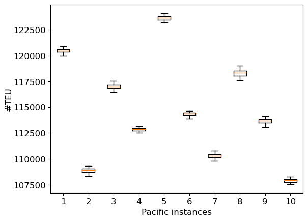
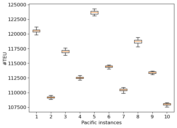
Before comparing the different approaches, we first analyze the behavior of the proposed incomplete method. First of all, our experiments have shown that the criterion to be optimized does not influence the time or quality of the results obtained. As the trends are often similar and due to lack of space, we will not present the results for each criterion considered hereafter. Such a result is not surprising since the criterion plays a minor role in Algorithm 1, impacting only line 10. Then, our method is relatively robust. Indeed, it can be observed that from one execution to another, the results are substantially the same, with a standard deviation of at most 4.3% in very rare cases and less than 1% in general. Figure 7(a) presents, for example, the dispersion of the values of the best solution for each of the ten Pacific instances when maximizing the quantity of transported commodities at the tactical level for one restart and 250 trials. Figure 7(b) does the same for 25 restarts and 10 trials per restart.
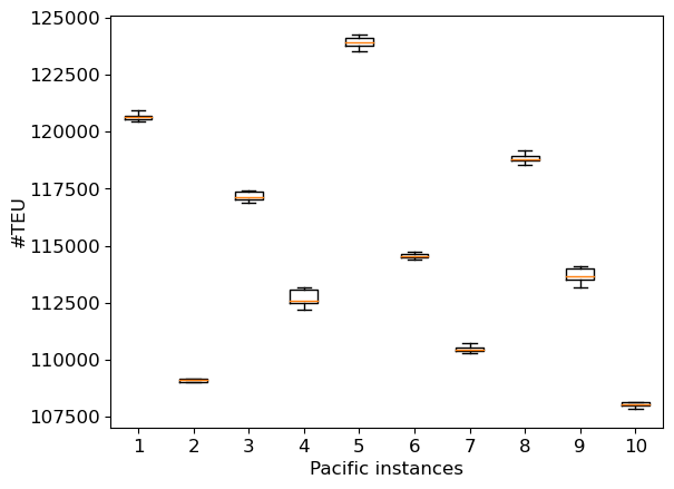
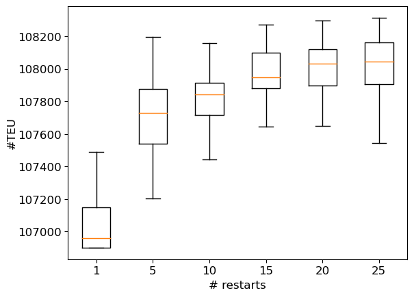
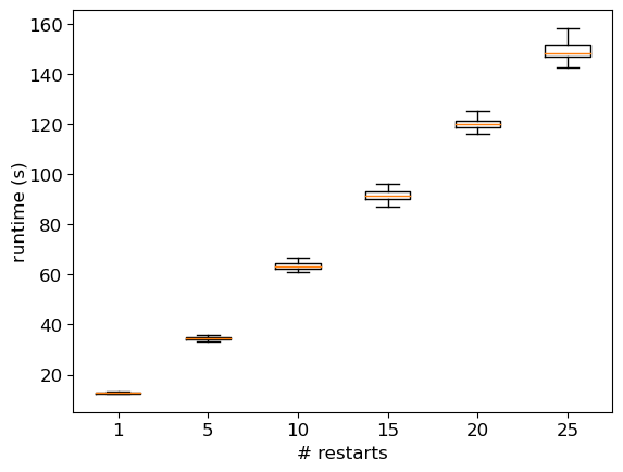
Next, we measure the impact of the number of trials by looking at the trial (out of 250) on which the best solution is found. Figure 8(a) presents the number of instances for which the best solution is found in a given interval of trials for a single restart. We consider here both tactical and operational instances. Clearly, for instances from Baltic, WAF and Mediterranean, whatever criterion, a number of trials of about 10 turns out to be relevant in most cases. For Pacific instances, it would seem that 50 trials would be more appropriate. As the runtime increases with the number of trials, the value 10 can generally be considered as a good trade-off between the runtime and the quality of the obtained solution. Then, we measure the impact of the number of restarts by looking at the run out of 25 on which the best solution is found. Figure 8(b) presents the number of instances for which the best solution is found in a given interval of restarts for 10 trials per restart. It appears that few restarts are often enough to obtain a good-quality solution. Again, the Pacific instances require an extra effort compared with those of other families. Indeed, the best results often require a number of restarts greater than 10. This can be explained by the size of the instances (the largest considered here), but also by the reduced number of iterations used here. Using 50 trials instead of 10 does imply a significant change (see Figure 7(c)). Figures 7(d) and (e) provide the dispersion for the quality of the solution and the runtime when maximizing the quantity of transported commodities for the instance Pacific_9 (at tactical level). We can observe a slight improvement in the quality when the number of restarts increases. Here, a 1% improvement in solution quality requires a 9-fold increase in runtime. So, using a small number of restarts seems to be a good trade-off between runtime and solution quality when solving the problem of cargo routing at tactical level, as such a problem will need to be solved a large number of times. In an operational context, focusing on profitability would require to spend more time on problem-solving, which would involve using the method with several dozen restarts.
 |
 |
| (a) | (b) |
 |
 |
| (c) | (d) |
 |
|
| (e) | (f) |
| Tactical level | Operational level | |||||
| TEU | Revenue | Benefit | TEU | Revenue | Benefit | |
| Baltic | 39 / 38 | 40 / 40 | 40 / 40 | 39 / 38 | 40 / 40 | 40 / 40 |
| WAF | 40 / 40 | 40 / 40 | 40 / 40 | 40 / 40 | 40 / 40 | 40 / 40 |
| Mediterranean | 35 / 39 | 34 / 34 | 0 / 0 | 36 / 39 | 36 / 30 | 0 / 0 |
| Pacific | 0 / 0 | 0 / 0 | 0 / 0 | 0 / 0 | 0 / 0 | 0 / 0 |
| Total | 114 / 117 | 114 / 114 | 80 / 80 | 115 / 117 | 116 / 110 | 80 / 80 |
 |
 |
| (a) | (b) |
6.3 Comparisons of the Different Approaches
6.3.1 Tactical level
First, we consider the tactical level where the cargo routing problem is used as a liner network design step. The aim is to evaluate the quality of the network produced according to a given criterion, such as the number of TEUs transported or the revenue/benefits generated. It should be noted that network design as a whole is beyond the scope of this paper.
| (a) | (b) |
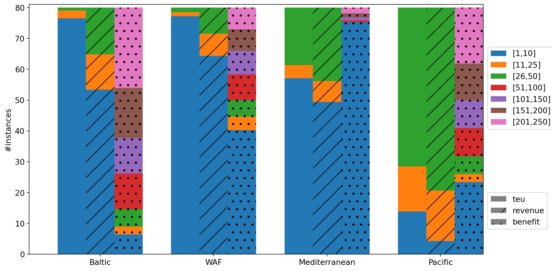
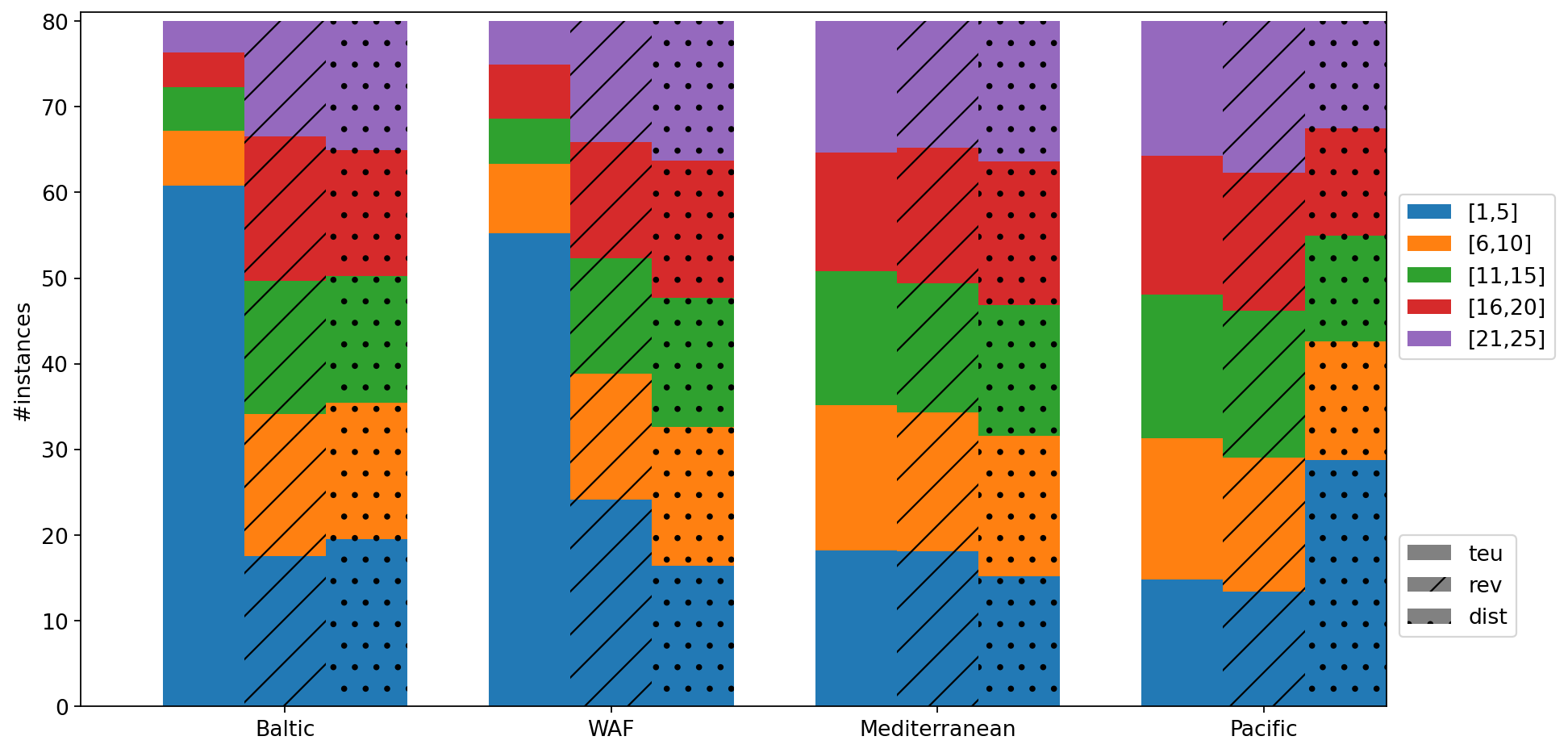
We first compare the and models. These two models are relatively close in terms of performance. Model optimally solves 114 instances compared to 117 for model when maximizing the quantity of transported commodities. For the two other criteria, both models optimally solve the same number of instances. Whatever the considered criterion, it turns out that, in general, instances based on Baltic and WAF are optimally solved. These instances are the smallest and correspond to feedering rotations (i.e. short rotations intended to supply main lines). In contrast, for instances based on Pacific (i.e. general instances integrating feedering and main lines), after one hour, the solver is still searching for the optimal solution, regardless of the model considered. We have observed that, most of the time, the last best solution is found around the time limit. This means that the solver has not yet begun the proof of optimality. Finally, we can note that maximizing the benefits (with a more complex objective function) seems to make the problem harder to solve. In particular, we can note that no Mediterranean instance is solved optimally.
If we compare the solving runtime for each model on instances which are optimally solved (see Figure 9(a)), we note that the solving is often faster with than with . However, if we consider the quality of the best found solution for the other instances, generally, finds slightly better solutions whatever the criterion. Nevertheless, the gap between the two models does not exceed 3% and it is often less than 1%.
| (a) | (b) | (c) |
Now, we consider the incomplete method and compare the quality of the solution it finds with the best solution found by one of the two models. Figure 10 allows estimating the quality of the solutions found by comparing the result of the incomplete search with the best solution found by one of the two models for all the considered criterion. We consider here 25 restarts and 10 trials per restart. The reported result for the incomplete search is the worst result found over the 50 runs performed for each instance. By doing so, we want to assess the quality of our incomplete approach in the worst case333Considering the best result over the 50 runs would only slightly improve the results, as the quality dispersion is low (see Figure 7).. This comparison shows that the incomplete method often obtains results close to those of a complete approach. We can see that, for some Baltic instances, the incomplete method performs slightly less well when maximizing the revenue or the benefits. This corresponds to instances for which the number of routes per commodity is reduced, making it more difficult for the incomplete method to find a good solution. Whatever the criterion, a similar trend can be observed for some Pacific instances with the same explanation. In terms of runtime, it takes a maximum of around 170 seconds for 25 restarts and 10 trials per restart for the largest instances, whereas Or-Tools systematically reaches the time-out for these instances although it uses 16 cores compared with one for the incomplete method. The incomplete method therefore delivers quality results in a reasonable time whatever the considered criterion. We can see from Figure 10(f) that a reasonable number of restarts and trials can do better, in some cases, than a complete approach, and that increasing the runtime still further does not lead to a significant improvement in results.
6.3.2 Operational use
We consider the case where the cargo routing problem is used in an operational context. At this stage, the network has already been built, i.e. the rotations have already been defined and a specific type of vessel is associated with each of them. In this case, the cargo routing problem is used to decide how commodities should be routed within the network. While this use can be seen as a special case of the tactical level, it does not make the solving easier. On the contrary, reducing the possible vessel types to just one per rotation further constrains the problem. As a result, we can note that model the model solves slightly fewer instances optimally. Beyond that, the trends observed for the tactical level remain valid and reinforce the interest of the incomplete approach.
It should be noted that these experiments were carried out with at most two splittings of each commodity, to enable comparison between the complete approaches and our incomplete method. Increasing the number of splittings significantly increases the difficulty of the problem when solved with a complete search. In contrast, our incomplete method can divide commodities into as many parts as desired without any noticeable increase in time. It is therefore better suited to use in real-life conditions, in particular to enable shipowners to achieve good values for quality indicators such as vessel filling factor.
7 Conclusions and Perspectives
In this paper, we have proposed two CP-based models for solving the cargo routing problem, as well as an incomplete method. The results we have obtained show the difficulty of optimally solving the cargo routing problem with a complete approach and so highlight the practical interest of incomplete methods such as the one we propose. This latter turns to be robust and provides relevant solutions within a very reasonable runtime whatever the criterion we consider. Our results also point out the difference in difficulty depending on the optimization criterion considered or the nature of the instances (feedering or general). On this latter point, a possible improvement for general instances would be to processes feedering and main line rotations separately.
References
- [1] R. Agarwal and Ö. Ergun. Ship Scheduling and Network Design for Cargo Routing in Liner Shipping. Transportation Science, 42(2):175–196, 2008. doi:10.1287/trsc.1070.0205.
- [2] J. F. Álvarez. Joint routing and deployment of a fleet of container vessels. Maritime Economics & Logistics, 11(2):186–208, 2009. doi:10.1057/mel.2009.5.
- [3] M. Ameln, J. S. Fuglum, K. Thun, H. Andersson, and M. Stålhane. A new formulation for the liner shipping network design problem. International Transactions in Operational Research, 28(2):638–659, 2021. doi:10.1111/itor.12659.
- [4] B. D. Brouer, G. Desaulniers, C. V. Karsten, and D Pisinger. A Matheuristic for the Liner Shipping Network Design Problem with Transit Time Restrictions. In Computational Logistics - 6th International Conference, ICCL, volume 9335 of Lecture Notes in Computer Science, pages 195–208. Springer, 2015. doi:10.1007/978-3-319-24264-4_14.
- [5] B. D. Brouer, J. F. Álvarez, C. E. M. Plum, D. Pisinger, and M. M. Sigurd. A base integer programming model and benchmark suite for liner-shipping network design. Transportation Science, 48(2):281–312, 2014. doi:10.1287/trsc.2013.0471.
- [6] M. Christiansen, E. O. Hellsten, D. Pisinger, D. Sacramento, and C. Vilhelmsen. Liner shipping network design. European Journal of Operational Research, 286, 2020. doi:10.1016/j.ejor.2019.09.057.
- [7] D. F. Koza. Liner shipping service scheduling and cargo allocation. EJOR, 275, December 2018. doi:10.1016/j.ejor.2018.12.011.
- [8] Y. El Ghazi, D. Habet, and C. Terrioux. A CP Approach for the Liner Shipping Network Design Problem. In CP, pages 16:1–16:21, 2023. doi:10.4230/LIPICS.CP.2023.16.
- [9] M. Giovannini and H. Psaraftis. The profit maximizing liner shipping problem with flexible frequencies: logistical and environmental considerations. Flexible Services and Manufacturing Journal, 31, September 2019. doi:10.1007/s10696-018-9308-z.
- [10] C. V. Karsten, B. D. Brouer, G. Desaulniers, and D. Pisinger. Time constrained liner shipping network design. Transportation Research. Part E: Logistics and Transportation Review, 105:152–162, 2017. doi:10.1016/j.tre.2016.03.010.
- [11] S. Lee, T. Boomsma, and K. Holst. Approximate dynamic programming for liner shipping network design. Annals of Operations Research, pages 1–40, July 2024. doi:10.1007/s10479-024-06106-1.
- [12] Q. Meng, S. Wang, H. Andersson, and K. Thun. Containership routing and scheduling in liner shipping: overview and future research directions. Transportation Science, 48(2):265–280, January 2014. doi:10.1287/trsc.2013.0461.
- [13] R. Neamatian Monemi and S. Gelareh. Network design, fleet deployment and empty repositioning in liner shipping. Transportation Research Part E: Logistics and Transportation Review, 108, July 2017. doi:10.1016/j.tre.2017.07.005.
- [14] J. Mulder and R. Dekker. Methods for strategic liner shipping network design. European Journal of Operational Research, 235:367–377, June 2014. doi:10.1016/j.ejor.2013.09.041.
- [15] S. Ozcan, D. Eliiyi, and L. Reinhardt. Cargo allocation and vessel scheduling on liner shipping with synchronization of transshipments. Applied Mathematical Modelling, 77, July 2019. doi:10.1016/j.apm.2019.06.033.
- [16] L. B. Reinhardt and D. Pisinger. A branch and cut algorithm for the container shipping network design problem. Flexible Services and Manufacturing Journal, 24(3):349–374, 2012. doi:10.1007/s10696-011-9105-4.
- [17] F. Rossi, P. van Beek, and T. Walsh. Handbook of Constraint Programming. Elsevier, 2006.
- [18] A. Santini, S. Ropke, and L. M. Hvattum. A comparison of acceptance criteria for the adaptive large neighbourhood search metaheuristic. J. Heuristics, 24(5):783–815, 2018. doi:10.1007/S10732-018-9377-X.
- [19] P. Shaw. Using constraint programming and local search methods to solve vehicle routing problems. In CP, volume 1520, pages 417–431, 1998. doi:10.1007/3-540-49481-2_30.
- [20] K. Thun, H. Andersson, and M. Christiansen. Analyzing complex service structures in liner shipping network design. Flexible Services and Manufacturing Journal, 29(3-4):535–552, 2017. doi:10.1007/s10696-016-9262-6.
- [21] P. Van Hentenryck and J.-P. Carillon. Generality versus Specificity: An Experience with AI and OR Techniques. In Proceedings of the National Conference on Artificial Intelligence, pages 660–664, 1988.
- [22] S. Wang and Q. Meng. Liner shipping network design with deadlines. Computers & Operations Research, 41:140–149, 2014. doi:10.1016/j.cor.2013.08.014.
- [23] S. Wang, X. Qu, T. Wang, and W. Yi. Optimal container routing in liner shipping networks considering repacking 20 ft containers into 40 ft containers. Journal of Advanced Transportation, 2017:1–9, January 2017. doi:10.1155/2017/8608032.