Disjunctive Scheduling in Tempo

Abstract
In this paper we introduce a constraint programming lazy clause and literal generation solver embarking ideas from SAT Modulo theories. A key aspect of the solver are Boolean variables with an associated semantic in difference logic, i.e., systems of binary numeric difference constraints or edges, making it particularly adapted to scheduling and other temporal problems. We apply this solver to disjunctive scheduling problems, where edges are used as branching variables, can be inferred via the edge finding rule as well as by transitivity reasoning, and can in turn strengthen propagation via temporal graph reasoning. Our experiments on job-shop scheduling show that a deep integration of these techniques makes our solver competitive with state-of-the-art approaches on these problems.
Keywords and phrases:
Scheduling, Constraint solvers, Clause-learningFunding:
Emmanuel Hebrard: supported by the ANR Project AD-Lib (ANR-22-CE23-0014); and the European Union’s Horizon Europe Research and Innovation program TUPLES No101070149.Copyright and License:
2012 ACM Subject Classification:
Applied computing ; Computing methodologies Discrete space searchSupplementary Material:
Software (Source Code): https://gitlab.laas.fr/roc/emmanuel-hebrard/tempo [23]archived at
Editors:
Maria Garcia de la BandaSeries and Publisher:
1 Introduction
Constraint solvers are constantly evolving. In particular, even tough some restricted form of nogood learning had been used in CP for a long time [19, 43], conflict-driven clause learning (CDCL) has had a significant impact on the design of constraint solvers. Bacchus and Katsirelos proposed to compute explanations of constraints in order to apply the principles of CDCL on constraint programs [25, 26]. Most hybrid CP/SAT solvers now implement the approach known as Lazy Clause Generation (LCG) [17, 36]: domains (and domain changes) are mapped to logical literals (including membership and bound literals), and constraints are propagated using dedicated algorithms as in CP although they generate explanation clauses in order to apply CDCL’s conflict analysis method. However, even though there are successful and established LCG solvers such as Chuffed [12], their implementation choices are less grounded than in pure CP solvers such as ACE [31], Choco [40, 41]111Note that recent versions of Choco also implements clause learning. or Gecode [44], and questions about their design remain open.
We introduce Tempo, yet another CP/SAT hybrid solver whose implementation of numeric variables is inspired from difference logic. This design choice makes it particularly suited for temporal and in particular scheduling problems. For instance, similar approaches have been shown to be very efficient on flexible job-shop [45] or on problems with reservoir resources[46], although such approaches are not limited to this domain. We discuss state-of-the-art solvers for this type of problems in Section 3 where we argue that in many cases the gains in performance came together with a significant complexity growth, such as the recourse to portfolios of algorithms. The overall architecture of Tempo, described in Section 4, is on the contrary relatively simple. One of its key aspects is that bound literals are purely lazy, that is, a literal is created in a branch of the search tree only when necessary and it “exists” in the data structure only in the subtree rooted at this branch. The solver Aries [6, 7] is built on the same or extremely similar ideas. However, Tempo implements constraint propagation, including global constraints via a constraint queue with configurable priority while Aries is restricted to a few simple constraints. The key differences with respect to Aries are described in Sections 5 and 6.
2 Background
In this section we briefly introduce the necessary background on Boolean Satisfiability (SAT), hybrid CP/SAT solvers, Difference Logic and scheduling.
2.1 Algorithms for Boolean Satisfiability
The Satisfiability problem is to decide if there exists an assignment of a set of atoms such that a propositional logic formula evaluates to true, that is, whether there exists a solution to: . We shall use the symbol to denote both the Boolean variable and the positive literal standing for this variable being true, while is the negative literal, standing for this variable being false. It is often assumed that the formula is in Conjunctive Normal Form (CNF). A CNF is a conjunction of clauses, i.e., a disjunction of literals.
Conflict-driven Clause Learning (CDCL) solvers [34] make branching decisions as other tree search algorithms, by adding an arbitrary new true literal to the formula. However, when encountering a failure, instead of undoing the most recent decision, a conflict clause, or nogood, is generated and added to the clause set. Let be the list, in chronological order, of literals currently true in some branch of the search tree, let be the rank of literal in and let the explanation for be the clause that unit-propagated (and we call the reason for ). Conflict analysis usually computes a conflict clause with a unique implication point (UIP) whose rank is higher than or equal to that of the last decision. Let a conflict set be a conjunction of literals that entails unsatisfiability of the formula , i.e., such that . The conflict set is initialized as the negation of the clause that triggered the failure. Then the literal with maximum rank is removed from and replaced by its reason until exactly one literal in has a rank superior or equal to that of the most recent decision (this literal is the first UIP, i.e., 1-UIP). This process is called conflict-driven clause resolution.222We define it using conflict sets because it is more intuitive and convenient, however, those are indeed resolution steps when adopting the clausal view. Then, every branching decision whose rank is higher than the highest rank of any literal in but the 1-UIP is undone, the conflict clause is added to the formula, and unit-propagation infers the negation of the 1-UIP literal.
2.2 Hybrid Solvers
Hybrid CP-SAT solvers work on the same principle, with two key differences. Firstly, there is a mapping between Boolean literals and restriction events on the domains of numeric (often integer) variables. For instance, a literal may stand for the assignment event and to the removal event . Secondly, arbitrary constraint propagation algorithms can be used as well as clauses to infer new true literals. In order to use conflict analysis as described above, general constraints must be able to produce explanation clauses. Given a literal inferred by some constraint propagation algorithm in a search state defined by the set of true literals , an explanation clause is a clause entailed by the model and such that unit-propagation on produces the true literal . The name Lazy Clause Generation comes from the fact that explanation clauses are generated during search rather than proactively as an encoding. However, this should not be confused with another type of laziness: explanation clauses can be generated during constraint propagation, or in a true “lazy” way, only when we want to replace a literal in the conflict set with its reason. In Tempo the two options are used, depending on the constraint.
2.3 Difference Logic
Satisfiability Modulo Theories (SMT) solvers decide the satisfiability of formula of the form with a propositional logic formula whose atoms have a semantic in an underlying theory. Difference Logic is a fragment of linear arithmetics where atoms stand for binary difference constraints of the form with and a constant.
The duality between shortest path and systems of difference constraints is well know [4]. A conjunction of difference logic constraints can be mapped to a temporal network, i.e., a directed graph with one vertex per numeric variable, and a labeled edge for every difference constraint . The system is satisfiable if and only if does not contain any negative cycle, and the difference constraint is entailed by if and only if the length of the shortest path from to in is less than or equal to . For this reason, we shall refer to difference constraints as edge in this paper.
Given the set of edges that appear in a formula, and given a subset of true edges (edge literals assigned to “true”), a difference logic reasoner is expected to decide if is consistent. If so, it should produce the set of edges entailed by , along with their explanations. If not, it should produce an explanation for the inconsistency. It is possible to compute all the entailed edges in polynomial time, by computing all-pair shortest paths in the graph with e.g., the Floyd-Warshall algorithm. State-of-the-art implementations do not compute the full transitive closure. Instead, when a new true edge is added to the system, only the edges that appear in the formula and have become entailed by the system are computed. This computation can be done incrementally, by maintaining a potential function and using Dijkstra’s algorithm, after relabeling the edges in the same way as in Johnson’s algorithm [13, 16].
2.4 Scheduling
The problem of scheduling tasks under resource constraints has been an extremely successful domain for constraint programming. We are given a set of tasks , where is defined by an interval of time of possibly variable length ; where denotes the start time of task ; and where is its end time. Tasks can be subject to precedence constraints, set between their start or end times. They can also be subject to resource constraints. In this paper we consider only disjunctive constraints, stating that two tasks using the same resource may not overlap. Difference logic captures well these problems since precedence constraints are edges and the NoOverlap constraint (also referred to as disjunctive or unary resource) is defined a 2-CNF whose atoms are edges:
| (1) |
Moreover, this formulation should make it clear that if all difference logic atoms are assigned a truth value, and if the resulting difference system is consistent, then the problem is satisfiable. Indeed, all constraints (precedences and resources) are defined exclusively using difference logic atoms. Therefore, if we maintain the consistency of the difference logic system, there is no need to branch on start times, end times or durations in the search tree. In this paper we only consider problems where the objective function to minimize is the maximum of all the end times (i.e., the makespan), although several other objectives are of interest.
3 Related Work
IBM’s CP Optimizer [29] has been considered as the state of the art on a range of scheduling problems for a long time. It is a commercial toolkit, its code is not open and if there is a significant amount of literature by various contributors, it is difficult to know with a high degree of certainty which techniques are used. However, the main components are described in [29]. With respect to constraint propagation, the default parameters are not known, but it is safe to assume that most if not all propagation rules for the NoOverlap constraint are implemented in CP Optimizer, and may be switched on or off during search or at preprocessing. Moreover, CP Optimizer uses the idea of gathering edges into a temporal network that can be used to make inference. Using Bellman-Ford on this graph to propagate the bounds of temporal variable is equivalent to using classic constraint propagation on precedences except that negative cycle can be found more quickly on very large domains. Although this is not confirmed in [29], we believe that it very likely uses this technique in conjunction with resource constraints to adjust the bounds of temporal variable in a similar way as we describe in Section 4.2, since these ideas were described in [27]. A significant effort has been given to the default search strategy. Large neighborhood search [47] is used to quickly find high quality solutions. Neighborhood selection (among a portfolios) as well as completion strategies selection relies on machine learning and some adaptive criterion [28]. When trapped in local minima the default strategy switches to Failure-Directed Search (FDS) [54]. In this strategy, branching choices are binary splits on the tasks’ start times. Moreover, it implements a rather complex system of rating for the choicepoints, with similarities to impact-based search [42]. It can also be compared to the notion of weight used in the weighted-degree heuristic [8] or of the activity used in the VSIDS heuristic [35], since it tries to focus on (and select choicepoints leading to) failures. CP Optimizer does not use clause-learning, however FDS includes storing and propagating nogoods from restarts [32]. Finally, it uses a limited form of strong branching [2] by propagating both branches of a subset of binary choicepoints before actually making a branching choice. This technique is used only on a subset of promising choicepoints and applied only near the root of the search tree. Google’s OR-Tools [38] implements many of the features in CP Optimizer, including the integration of a simplex algorithm, dedicated scheduling algorithms from operation research and CP and large neighborhood search as well as other local search techniques [14]. However, unlike CP Optimizer, it is an hybrid CP/SAT solver implementing lazy clause generation techniques taking inspiration from Chuffed. OptalCP is a commercially released constraint solver, which shares many traits with CP Optimizer, and a focus on implementation and design choices geared toward a more efficient use of CPU and caches [53]. It was shown to be even more efficient than CP Optimizer, in particular on disjunctive scheduling problems.
Those three toolkits are designed to be usable by non-experts. Therefore, they typically implement highly complex search and parameter tuning strategies as well as inprocessing techniques in order to be robust, instead of leaving these choices to the user. Finally, they are designed to get the most out of multiprocessing, through the use of portfolios of algorithms and communication between threads. This approach has proven extremely effective and lead to several successful applications. On the other hand, simpler approaches have been shown to be very effective on disjunctive scheduling problems: although using a pure CP solver (Mistral), an early approach using the observation that we only need to branch on edge variables was used with success on disjunctive scheduling problems [20]. It was in particular the first to solve every Open-shop instance in Brucker’s data set [9] to optimality [21]. Since this approach did not use any dedicated resource constraint propagation algorithm, its efficiency had two main explanations: it explores a search tree whose choicepoints are edges, as explained above; and the weighted-degree heuristic was shown to be very effective in finding the important variables to branch on. An extension of this method with a limited form of clause learning was later shown to be slightly more effective on job-shop benchmarks [48]. More recently, a very efficient solver, called Aries, based on the same principles, but implementing clause-learning as well as all the standard CDCL techniques was proposed. [7] This approach used many of the same ideas on difference logic and edges developed in this paper. With respect to the constraint model and inference mechanisms, as far as we are concerned with disjunctive scheduling, Aries can be seen as Mistral plus clause-learning and the approach we propose, Tempo, can be seen as Aries plus global constraints. The variable heuristics are different though working on the same principles: Aries uses learning-rate [33] as default heuristic while the version of Tempo used in our experiments variable state independent decaying sum [35].
4 Principles of the Solver
The key difference between a pure CP and a hybrid CP/SAT solver is that in the latter, the information about the current domains, and its changes thereof, must be encoded in atomic referenceable literals. We detail the different types of literals in Tempo in Sections 4.1 and 4.2, and then we show how they affect a core technique in SAT solver: unit-propagation.
4.1 Variables and Literals
There are two primitive types of variables in the solver: Boolean and numeric variables. The domain of a numeric variable is defined by its lower and upper bounds. Bound literals are constraints of the form . We use signed variables so that bound literals are all in the canonical form of difference logic constraints ( is written ), and so that a smaller right-hand side always corresponds to a tighter literal. We say that is active if it was created (e.g. by constraint propagation) at a decision level lower than or equal to the current one in the same branch. In other words, a literal can be true without being active, if there is an active literal with . For every signed variable, the list of active literals maintained in decreasing order of their right-hand sides. For instance, if the lower bound of a numeric variable changes (to take the value ) because of constraint , the literal is inserted at the end of the list for and its explanation is . Some solvers [26, 17] support lazy bound literal generation. A possible implementation is essentially equivalent to adding new Boolean variables during search with a bound semantic attached to it. This means that the corresponding Boolean variable must live as long as a clause involves such a literal. More generally, adding such literals during search is easy, however, making sure that the number of literals does not grow too large is difficult. Therefore, in Tempo, much like in Aries, the literal is not linked to any Boolean variable. It is created when the domain of variable changes accordingly, and no longer exists when backtracking over that decision level in the search tree. However, this incurs a cost when accessing the informations attached to such a literal. For instance if one wants to access the explanation for , one must search for the highest value of such that the literal is currently active. Since entails , its explanation is also valid333Note that cannot be in the explanation of because it would entail that a literal with is active but that would contradict is the highest such value.. Similarly, if the literal is inferred e.g., by constraint propagation, unit-propagation algorithm would access the list of clauses that watch it in constant time. This is impossible if we do not allocate any memory for literals that are not active. Our implementation of the watched literals data structure is discussed in Section 4.3.
4.2 Temporal Network
As in SAT Modulo Theories solvers, Boolean variables may be given a semantic in difference logic, i.e., each literal of a Boolean variable can be associated to an edge: . The negative literal can stand for the negation of the edge (). However, we allow for the positive and negative literals of the same variable to be associated to any edges, or no edge at all. This is useful to represent a binary disjuncts with a single variable, e.g.:
| (2) |
The binary disjunct in Eq. 2, stating that tasks and do not overlap can be represented with a single variable with and . This is also useful for optional tasks, where we might want that a Boolean variable implies an edge, but its negation leaves the numeric variable free.
The difference logic system in implemented in Tempo uses a reversible directed graph . When the literal is set to true, the edge is directly added to the difference logic system, modeled by the arc in . Our implementation differs from the method described by Cotton and Maler [13] in the following ways: Firstly, as explained by Feydy et al., in typical constraint problems, many more bounds literals are propagated than edge literals, and hence it is important to have a dedicated procedure for each type [16]. Moreover, since bounds literals are generated lazily, they do not necessarily appear in the formula prior to search. We use the common approach to have a distinguished vertex standing for the constant in the temporal network. This vertex is connected to every other numeric variable, however implicitly. That is, if is the tightest true upper bound literal for variable , then everything works as if the arc was in the graph, i.e., the difference constraint , and similarly, indicates the arc . Those arcs are not actually added to avoid having several arcs between the same vertices. Therefore, given the set of edges that appear in the constraint program and a subset of true edges, for each new edge , the reasoner achieves three tasks: decide consistency; compute the set of bounds literals entailed by ; and compute a set of entailed (non-bound) edges.
As in [16], given a new arc , the first two tasks are done via two calls to a shortest path algorithm. Let be the length of the shortest path from the origin () to , and be the length of the shortest path to the origin from in . The bound literals and are entailed by . In other words, all the upper (resp. lower) bound updates can be done by computing all the shortest paths from (resp. to) in . Since a shortest path can have changed only if it goes through the arc this can be done by one call from and another from in the converse graph. Notice that the shortest path algorithm can be stopped early when reaching a vertex whose shortest path from (resp. to) has not changed. Our approach has a worse time complexity than those described in [13, 16] because we use a version of Dijkstra with a simple FIFO queue but where the same vertex can enter the queue more than once. The worst-case time complexity of this algorithm is the same as Bellman-Ford. However, as opposed to Dijkstra’s algorithm, it can work directly on graphs with negative arcs and is efficient in practice when the new edge does not entail many bound updates. If the shortest path from the origin to is updated to a strictly lower value (say ) and is its predecessor on the path, via the arc , then the literal is inferred, and its explanation is:
| (3) |
Moreover, there is a negative cycle if and only if the shortest path from to is updated in the first call, and the explanation is the set of edges in the negative cycle.
Finally, the main difference with respect to [13, 16] concerns the third task: we do not infer all the edges entailed by the current set of true edges. Indeed this requires to either store all the shortest paths and hence quadratic space, or to run the shortest paths algorithms as explained above, but without the early stop condition. Even though the worst-case time complexity is the same, it makes a significant difference on dense precedence networks. In our experiments this turned out to be too costly, and instead we compute only a subset of entailed edges. The rule to infer that the edge is false corresponds to the standard propagation rule for binary disjunctions in existing scheduling models. Within the difference logic system implemented in Tempo, the rule is as follows:
| (4) |
Indeed the following difference logic sentence is unsatisfiable
| (5) |
since it can be reduced to .
For every edge in the difference logic system, there is a propagator that watches the lower bound literals of the numeric variable and the upper bound literals of the , and triggers exactly as shown in Eq. 4 to produce the literal . The explanation can be:
| (6) |
We use a slightly improved explanation. Assume that the most recent bound literal is . Then the explanation for is:
| (7) |
Since we only need and this explanation is therefore more general.
4.3 Unit-Propagation of Bound Literals
Since bound literals are generated lazily, we cannot have constant-time access to all data structures storing information on literals. Bound literals are simply stored in order, with one list for upper bounds and another list for lower bounds. Therefore, the current lower and upper bound of a given numeric variable can be accessed in constant time. However, accessing the explanation for a given literal requires to traverse the list of upper bounds literals for the variable . This could be done by binary search, however, since conflict analysis usually does not explore literals beyond the current decision level, we chose to use a linear search starting from the most recent bound instead. Since conflict analysis is not as time consuming as constraint propagation, this is not a very important issue.
On the other hand, unit-propagation represents a significant proportion of the total runtime, and the watched-literal data-structure [35] must be adapted. In the standard method, we have a list of watcher clauses for every literal, containing every clause that watches it (every clause watches two of its literals). We use the standard implementation when the watched literal is Boolean. Instead, for bound literals, we have an array indexed by signed numeric variables, i.e., is the watch-list for the upper bound of and is the watch-list for its lower bound (see example in Figure 1). This array maps each signed variable to a list containing pairs where is a numeric value and is the list of clauses currently watching the literal . Those pairs are ordered by increasing value of . When a literal (resp. ) becomes true, we scan the list (resp. ). When encountering a pair with we know that the clauses in and in all the list after do not need to be unit propagated since they watch a literal weaker than , and hence no more propagation can occur.
However, the list must be maintained sorted. Therefore, the additional cost of this data structure comes when moving a clause from a watch list to another watch list. That is, suppose that the literal watched by clause is falsified. If the clause contains an unwatched, unassigned literal (say ) then must be removed from , which can be done in constant time, and added to the list . This can also be done in constant time, however, finding the list within takes a time linear in the size of . In other words, the insertion cost will increase linearly with the number of different bound literals currently watched for the same numeric variable.
5 Edge-Finding: propagation and explanation
The standard Edge-Finding [10] rule for the NoOverlap constraint (see Eq. 1) is implemented in Tempo. We write for the earliest start time of a task , that is, the lower bound of the start time variable at a given point in search, and for its latest completion time, i.e., the upper bound of . Moreover we extend this notation to set of tasks, with , and
The overload rule is a sufficient condition for unsatisfiability of :
| (8) |
The Edge-Finding rule uses Eq. 8 to infer precedence relations, i.e., edges:
| (9) |
It “finds” the set of edges on the right-hand side of the consequence 9, which are entailed by the fact that if task is not the last one to be processed in the set , then the latest completion time would be too early to process all the tasks in . Since in the proposed framework we have variables for edges, we can directly set the edge to true. In standard implementations, however, this inference cannot be directly stored and instead the bounds of the numeric variables are adjusted accordingly via the two following rules:
| (10) | |||||
| (11) |
Notice that Eq. 10 is redundant when edges are assigned, although Eq. 11 is not, because it uses the fact that tasks in must all be completed before and they cannot overlap. This adjustment, however, is weaker than the propagation described in Section 6, and hence our implementation of Edge-Finding only assigns the corresponding edge literals.
Let such that Eq. 9 is triggered. For each , the edge can be explained by the following clause:
| (12) |
However, we use Vilím’s algorithm [51] for Edge-Finding, which does not explicitly keep track of a minimal set . For the sake of simplicity, we show here how to explain a failure of the overload rule (Eq. 8) as it is essentially the same construction in the general explanation.
One basic observation is that there are only non-dominated sets to consider in Equations 8 and 9 for a resource involving tasks: given some values for and we only need to consider the maximal set of tasks wholly within those bounds, and there are at most possible distinct values for and . Vilím’s algorithm goes one step further and achieves all these tests in time thanks to the Theta-Tree data structure. This algorithm explores tasks in non-decreasing latest completion times. Assume that tasks are numbered accordingly (i.e., so that implies ). Given task it computes the “elastic” approximation of the earliest completion time of sets of tasks . An replace Eq. 8 with:
| (13) |
Within the Theta-tree structure, the following recursion is used to compute the elastic earliest completion time of a set of tasks , from two disjoint sets such tasks in have lower earliest start times than tasks in (i.e., such that ):
| (14) |
There is one such set of tasks per node in the Theta-tree, with each leaf standing for a singleton set containing one task in , and internal nodes are computed using Eq. 14. In order to extract sound and minimal explanations, we keep track of an additional information in each node of the Theta-tree: the relevant earliest start time, that we write . For a leaf we have . Then we use the following recursion:
| (15) |
Then, from a set of tasks we can compute a potentially smaller explanation set: . The intuition is that when the earliest computation time of is computed in Eq. 14, if then the tasks in are irrelevant and hence can be removed from the explanation. Eq. 15 keeps track of this information. The following theorem essentially says that the set is a solution of Eq. 8, i.e, sufficient to entail a failure and explainable with Eq. 12.
Theorem 1.
For any node of the theta-tree corresponding to the set of tasks , the following equality is true:
Sketch of proof.
The full proof is given in appendix. We use an induction on the size of . There are two cases corresponding to the two sides of the recursion (Eq. 14). The child nodes and are strictly smaller than and hence they satisfy the induction hypothesis. Moreover the composition is straightforward when and only slightly more involved in the second case.
6 Edge Reasoning
All the edges, from the definition of the problem, from branching decisions, from the temporal network (Bellman-Ford or Eq. 4), and from Edge-Finding are stored in the temporal network. We discuss here the possibility of adding yet more edges from transitivity reasoning, and we show how we use all those edges to strengthen propagation on bound literals.
6.1 Transitivity
We do not use the strongest possible consistency in the difference logic reasoner since computing the full transitive closure can be very costly. However, within the scope of a NoOverlap constraint on , we can compute the transitive closure on the edge variables. The transitivity propagation rule is straightforward, and self-explained:
| (16) |
We use a reversible graph data structure for efficient access to the list of current successors and predecessors of a task. When an edge becomes true we add the edge for each successor of , and for each predecessor of .
6.2 Bounds adjustment
The graph of precedences between tasks sharing the same resource can be leveraged to infer further propagation. This has been described in the more general context of cumulative resources [27], however, we focus here on the simple case of a disjunctive resources and use an algorithm described in Vilím’s Ph.D. thesis [52]. Suppose that we have a task and a set of tasks all requiring the same resource, and such that for each , is true. Then, although neither the precedences nor the NoOverlap relation can conclude, the tasks in cannot overlap because of the disjunctive resource, and hence we have:
| (17) |
There is as many non-dominated sets to consider than successors of . Indeed, for any let be the task with highest . The set containing every successor of whose latest completion time is lower than or equal than is such that and .
Alg. 1 is not identical, but essentially equivalent to Vilím’s. It first sorts the tasks by increasing latest completion time. Now, consider a literal created for task at Line 1. Task is a successor of and each successor whose latest completion time is less than has been explored earlier (because of the ordering). Therefore, contains the sum of their durations. Alg. 1 runs in time linear in the number of true edges. It is sound because it applies the rule in Eq. 17, which is sound, and it is complete because we established that it goes through all the potentially non-dominated application of the rule.
7 Clause Minimization
Clause minimization is an important part of CDCL. It consists in detecting redundant literals in the conflict clause (see Section 2.1) and removing them to obtain a stronger clause.
Given a conflict set for the formula , the literal is said redundant if . A sufficient condition is that is not a decision and its reason is a subset of the conflict set , or that every literal in the difference is itself redundant. This recursion defines the implication graph, which, in the standard clause minimization algorithm, is explored up until encountering a decision or when a given depth is reached. In both of these cases, the literal is considered relevant (non-redundant). Otherwise, the exploration ended because all the ancestors of belong to and is redundant.
However, this procedure is not as simple in the context of lazy bound literal generation. Indeed, the definition of membership of a bound literal to a clause may have more than one definition. A trivial one is that the clause contains the literal . However, another possible definition is that the clause contains a literal such that . In this case the literal is a direct consequence of the clause, and hence this weaker definition of membership yields shorter clauses after minimization. However, one needs to be careful. Assume that Bellman-Ford infers the bound literal . Then it is explained by a 3-clause of the form (see Eq. 3). Moreover, suppose that the edge was inferred by Eq. 4. Then it has as explanation another 3-clause of the form with since the literal is “older” than (i.e., ). The implication graph for this example is shown in Fig. 2, where each vertex is a literal, and the set of direct predecessors (solid edges) of a literal corresponds to its explanation. The dashed edge is the “implicit” implication via the semantic of the bounds. Notice that it introduces a cycle in the implication graph.
Suppose that the conflict set (negation of the first UIP clause) contains the literals , and , with and . If we query the procedure sketched above for the redundancy of the literal , it would explore the ancestors of and finds they are all implied by the conflict set. As a result, it would wrongfully classify the literal as redundant and remove it from the conflict set.
Therefore, one cannot use the implication when checking the redundancy of literal . However, we can apply the following rule:
Proposition 2.
Let be a conflict set and let be an arbitrary conflict set obtained by conflict-driven clause resolution from .
If then,
Proof.
The proof is direct from the fact that (because conflict-driven clause resolution is correct), and because, .
Therefore, when Proposition 2 applies, is not redundant, but we can weaken it to in the conflict set, and hence strengthen the corresponding literal in the conflict clause to .
8 Experimental Results
We used three types of problems to benchmark our solver: job-shop scheduling, open-shop scheduling and job-shop with time lags. In all three problems there are machines and jobs each containing tasks. All machines are disjunctive resources. In job-shop scheduling, the sequence of the tasks in each job is fixed and each task requires exactly one of the machines. Job-shop with time lags are job-shop instances with the extra constraint that the interval between the end of any task and the start of the next task on the same job should be less than some value (in the data set it is set to either , , , , or times the average length of a task). Finally in Open-shop instances, the sequence in each job is a decision variable, or in other words, a job is a disjunctive resource in the same way machines are. We used well known data sets, whose detailed description is given in Table 4 in Appendix.
All experiments ran on a cluster of machines with 3 types of processors: Intel E5-2695 v3 2.3Ghz; Intel E5-2695 v4 2.1Ghz and AMD EPYC 7453 3.4Ghz. All the runs involving job-shop instances ran on the first type, open-shop instances on the second and job-shop with time-lags instances on the third, in order to ensure a fair comparison. We compared against the solvers Aries, CP Optimizer (version 22.11), OptalCP and OR-Tools. We did not run comparison with other solvers, although we quickly assessed the models for job-shop scheduling provided in the sources of Gecode and Chuffed and the results did not seem competitive. We used the following parameter setting for Tempo: the variable selection heuristic is VSIDS; the strategy to select clauses to forget uses literal activities from VSIDS; the value selection heuristic follows the choices that lead to the current best solution [5]; a straightforward insertion heuristic using a randomized mix of earliest start time and minimum slack is used to construct an initial upper bound; and no initial lower bound is implemented, besides the Edge-Finding rule. Some further numeric parameter setting were obtained by running Tempo on 8 instances (4 job-shop, 2 open-shop and 2 job-shop with time lags) and selecting the best out a few reasonable choices. We found that these parameters did not have a very significant impact: the clause minimization depth is set to , the decay value for VSIDS is set to , the ratio of forgotten clauses per restart is and a geometric restart policy is used, with a base limit of failures and a factor of .
For every solver, we used models of job-shop provided in their distribution, and hence we assume that they are reasonably well tuned for these standard instances. Aries, CP Optimizer and OptalCP also provide a default model for open-shop which we used in the same way. We implemented a model for job-shop with time lags by minimally changing the model for job-shop in all four solvers, and did the same for open-shop in OR-Tools.
OptalCP, however, uses two main strategies. The default one focuses on finding high quality solutions quickly and relies mainly on LNS, while the other focuses on optimality proofs and relies on FDS. Although the default strategy was remarkably efficient on job-shop, even proving optimality in many cases (see Table 3), it was unable to prove optimality in most other cases, and was much less efficient on job-shop with time-lags. Therefore, we report the results of OptalCP in Table 1 and OptalCP only in Table 3.
8.1 Comparison with the sate of the art
We ran every method on every instance with 10 distinct random seeds. Every run was stopped after 30 minutes of user time. We then grouped the instances into two categories “Easy” and “Hard”, where the former corresponds to instances solved to optimality by all five solvers in every run, and the latter contains all the remaining instances.
8.1.1 Hard instances
| instances | OR-Tools | Aries | CP Optimizer | OptalCP | Tempo | |||||
|---|---|---|---|---|---|---|---|---|---|---|
| #Opt. | Objective | #Opt. | Objective | #Opt. | Objective | #Opt. | Objective | #Opt. | Objective | |
| Jobshop Scheduling Problems | ||||||||||
| abz(30) | 0 | 674.0 | 0 | 671.5 | 8 | 675.7 | 0 | 679.0 | 2 | 671.6 |
| cscma(400) | 0 | 5690.7 | 0 | 5472.1 | 0 | 5364.9 | 0 | 6405.5 | 0 | 5287.1 |
| ft(10) | 10 | 1165.0 | 0 | 1165.0 | 10 | 1165.0 | 10 | 1165.0 | 10 | 1165.0 |
| la(20) | 10 | 1196.3 | 4 | 1199.3 | 19 | 1193.5 | 10 | 1200.0 | 13 | 1193.6 |
| rcmax(390) | 10 | 4354.3 | 90 | 4193.0 | 181 | 4190.2 | 40 | 4547.3 | 170 | 4180.7 |
| swv(150) | 10 | 2139.9 | 9 | 2132.2 | 34 | 2088.0 | 20 | 2293.8 | 39 | 2053.6 |
| ta(710) | 44 | 2652.4 | 134 | 2542.6 | 326 | 2528.6 | 54 | 2830.9 | 242 | 2553.0 |
| yn(40) | 0 | 928.0 | 0 | 921.5 | 0 | 931.0 | 0 | 938.5 | 0 | 921.4 |
| all(1750) | 84 | 3583.8 | 237 | 3452.5 | 578 | 3418.1 | 134 | 3876.1 | 476 | 3404.9 |
| Openshop Scheduling Problems | ||||||||||
| bru7(10) | 0 | 1048.6 | 10 | 1048.0 | 10 | 1048.0 | 10 | 1048.0 | 0 | 1048.0 |
| bru8(40) | 30 | 1014.9 | 40 | 1014.5 | 11 | 1018.1 | 40 | 1014.5 | 30 | 1014.5 |
| all(50) | 30 | 1021.7 | 50 | 1021.2 | 21 | 1024.1 | 50 | 1021.2 | 30 | 1021.2 |
| Jobshop Scheduling Problems with Time Lags | ||||||||||
| ft_1(10) | 0 | inf | 10 | 961.0 | 10 | 961.0 | 10 | 961.0 | 10 | 961.0 |
| la_0(280) | 10 | 2333.0 | 144 | 2344.3 | 40 | 2385.8 | 70 | 2439.9 | 119 | 2364.0 |
| la_0,5(300) | 0 | 1680.2 | 104 | 1570.4 | 50 | 1615.1 | 100 | 1613.6 | 79 | 1589.7 |
| la_1(290) | 9 | 1504.0 | 109 | 1355.1 | 139 | 1385.7 | 170 | 1374.3 | 97 | 1370.4 |
| la_2(30) | 11 | 895.4 | 29 | 904.7 | 30 | 904.7 | 30 | 898.3 | 30 | 904.7 |
| la_3(120) | 32 | 1552.8 | 73 | 1427.7 | 80 | 1427.2 | 70 | 1433.8 | 98 | 1418.2 |
| la_10(20) | 9 | 1196.5 | 5 | 1201.5 | 20 | 1194.0 | 10 | 1193.5 | 10 | 1194.6 |
| all(1050) | 71 | 1778.7 | 474 | 1669.2 | 369 | 1701.2 | 460 | 1712.7 | 443 | 1682.9 |
Results for hard instances are reported in Table 1. For each data set, the total number of runs is shown next to the data set name, then we report the number of proofs (#Opt.) and the average objective value (Objective). No solver is clearly the best on every data set.
On some instances of job-shop with time lags, OR-Tools does not find feasible solutions. The reason is simple: the cycles in the temporal graph make feasibility hard on this problem, even without upper bound. However, without upper bound, constraint propagation is ineffective and solvers are blind. Other solvers use some form of greedy initialization able to find a reasonable upper bounds to bootstrap search, which is crucial here. We believe that either OR-Tools simply does not run such greedy initialization, or that it sometimes fails to provide an initial feasible solution and hence this observation is not as noteworthy as one might think. However, the overall results are not as good as other solvers in general on these instances. It should also be noted that OR-Tools has been designed to be robust on a much wider range of problems (whereas other solvers are more focused on scheduling) and also to take full advantage of parallelism and is not as efficient in single-thread mode. We consider it beyond the scope of the paper to experiment using multi-threading.
The solver Aries, despite not using any dedicated propagator for the NoOverlap constraint ob-shop with time lags and tied for best on open-shop. In the case of Open-shop, there are only 5 hard instances in the whole data set, all from [9]. Methods that branch on edges and explore the search tree extremely fast have been shown to be efficient on those instances [21]. Moreover, the parameter that is probably the most important here is the variable selection heuristic. We ran Tempo without the NoOverlap propagators (Edge-Finding and Precedence-Disjunctive) since it is then very similar to Aries, with the main difference being the variable selection policy. The results of Tempo are still slightly worse on those instance than with them. We therefore believe that the explanation is related to the variable-selection policy. It is not as simple as simply the difference between learning-rate and VSIDS since we tried both in Tempo, and we did not notice much difference. However, there are many other decisions and parameters in the implementation of these heuristics (which set of literals should get their activity bumped on conflict, which value of decay should be used, etc.). On job-shop with time lags instances, we believe that the reason is mainly that the time lags constraints make the resource constraints comparatively less important to propagate than on classic job-shop or in open-shop. Indeed, Tempo without the NoOverlap propagators has results similar to those of Aries. However, Aries is clearly dominated by CP Optimizer and Tempo on job-shop, where stronger propagation is important.
CP Optimizer is extremely robust. Overall it produces more proofs than any other solver, and is clearly dominated only on open-shop. This is not surprising as CP Optimizer implements a large portfolios of techniques for scheduling problems and is finely tuned on these instances.
OptalCP is extremely fast. However, as discussed previously, it does not have the same adaptive search strategy as CP Optimizer, and hence it can be seen as two solvers. OptalCP is the best on open-shop but is clearly dominated by all other solvers on job-shop. On the contrary, OptalCP is the best on job-shop, but rarely proves optimality and is overall worse on open-shop and job-shop with time lags (see Table 3).
Tempo seems at least as robust as CP Optimizer, although it does not use any complex strategy to adapt the heuristics and parameters during search. If we include OptalCP, Tempo is second-best on all three problem types. Moreover, it is consistently within the best solvers in every data set, to the exception of the 10 largest Taillard’s job-shop instances, with 20 machines and, crucially, 100 jobs. In other words each of the 20 NoOverlap constraints involve 100 tasks and 4950 edge variables. In Tempo, the Edge-Finding propagator is used unconditionally and without any incremental aspect. As a result, the exploration speed drops dramatically on these instances. Whereas CP Optimizer finds the optimal solution with a proof on all 10 runs for each of these 10 instances, the best solution found by Tempo is very far from optimal. If we ignore those ten instances, the number of proofs is very close for both solvers (478 for CP Optimizer and 476 for Tempo), moreover the gap in average objective value is significantly larger (3300.1 for CP Optimizer and 3273.2 for Tempo).
8.1.2 Easy instances
| instances | OR-Tools | Aries | CP Optimizer | OptalCP | Tempo | |||||
| CPU | #Bran. | CPU | #Bran. | CPU | #Bran. | CPU | #Bran. | CPU | #Bran. | |
| Jobshop Scheduling Problems | ||||||||||
| abz(20) | 1.11 | 9236 | 0.29 | 4449 | 1.12 | 42660 | 0.33 | 27681 | 0.19 | 2487 |
| ft(20) | 2.97 | 20036 | 0.88 | 8900 | 2.24 | 69257 | 0.46 | 32846 | 0.46 | 3900 |
| la(380) | 20.61 | 78717 | 11.56 | 61186 | 6.62 | 190685 | 8.40 | 329783 | 3.64 | 15764 |
| orb(100) | 11.88 | 56344 | 2.72 | 23874 | 3.91 | 134998 | 1.23 | 87903 | 0.92 | 7197 |
| rcmax(10) | 192.82 | 577669 | 5.86 | 154845 | 0.21 | 10522 | 850.77 | 15743276 | 157.34 | 376972 |
| swv(50) | 46.23 | 205626 | 1.79 | 57660 | 0.39 | 15104 | 254.06 | 7267279 | 36.36 | 115931 |
| ta(90) | 220.20 | 605827 | 37.99 | 144237 | 90.42 | 2072631 | 27.17 | 745279 | 23.01 | 47046 |
| all(670) | 49.49 | 159276 | 12.32 | 64653 | 16.62 | 411337 | 40.28 | 1079388 | 10.37 | 30803 |
| Openshop Scheduling Problems | ||||||||||
| gp(800) | 0.51 | 8316 | 0.13 | 12687 | 1.31 | 53780 | 0.26 | 25409 | 0.19 | 5129 |
| bru(470) | 1.77 | 12197 | 0.88 | 8154 | 3.87 | 165362 | 0.39 | 29342 | 0.19 | 2091 |
| ta(600) | 4.17 | 46528 | 0.26 | 9497 | 0.52 | 15576 | 3.79 | 228003 | 0.91 | 6525 |
| all(1870) | 2.00 | 21552 | 0.36 | 10524 | 1.70 | 69567 | 1.43 | 91401 | 0.42 | 4813 |
| Jobshop Scheduling Problems with Time Lags | ||||||||||
| car(320) | 1.51 | 25667 | 0.30 | 5192 | 1.30 | 53948 | 0.25 | 25923 | 0.14 | 2007 |
| ft(150) | 12.89 | 81471 | 0.63 | 7446 | 6.11 | 192551 | 1.20 | 72274 | 0.60 | 4510 |
| la(1140) | 50.23 | 237217 | 11.86 | 71476 | 9.14 | 323321 | 4.26 | 261323 | 4.20 | 20275 |
| all(1610) | 37.07 | 180659 | 8.52 | 52336 | 7.30 | 257598 | 3.18 | 196922 | 3.06 | 15175 |
Results for easy instances are reported in Table 2. For each data set, the total number of runs is shown next to the data set name, then we report the average CPU time (CPU) and the average number of branching choicepoints explored (#Bran.).
The CPU time results are not easy to interpret. However, the number of explored choicepoints is interesting. Tempo very consistently explores the smallest subtree. Aries does not use costly propagators, and we believe that CP Optimizer and OR-Tools use them more parsimoniously. There are two data sets where Tempo explores more branches: “rcmax” and “swv”. However, the number of failures on these instance is still 4 times lower than for CP Optimizer. In fact, Tempo finds very poor initial solutions, and goes through many more improving solutions than CP Optimizer before reaching the optimal. Each one is found after very few failures, but many choicepoints are explored. We believe that LNS is key on these instances as well as on the large Taillard instances discussed earlier.
| solver | job-shop | open-shop | jsp with time lags | |||
|---|---|---|---|---|---|---|
| #Opt. | Objective | #Opt. | Objective | #Opt. | Objective | |
| OR-Tools | 84 | 3583.8 | 30 | 1021.7 | 71 | 1778.7 |
| Aries | 237 | 3452.5 | 50 | 1021.2 | 474 | 1669.2 |
| CP Optimizer | 578 | 3418.1 | 21 | 1024.1 | 369 | 1701.2 |
| OptalCP | 480 | 3391.4 | 0 | 1024.2 | 70 | 1724.0 |
| OptalCP | 134 | 3876.1 | 50 | 1021.2 | 460 | 1712.7 |
| Tempo | 476 | 3404.9 | 30 | 1021.2 | 443 | 1682.9 |
| Tempo | 485 | 3406.5 | 30 | 1021.4 | 466 | 1677.6 |
| Tempo | 117 | 3492.9 | 30 | 1021.6 | 460 | 1678.8 |
| Tempo | 460 | 3407.1 | 30 | 1021.3 | 446 | 1683.8 |
8.2 Ablation study
The second part of Table 3 gives the result on an ablation study on some aspects of Tempo:
The first observation is that the transitivity and temporal graph reasoning does not pay off. It helps on open-shop and with respect to the best objective on job-shop, but actually degrades the performances on job-shop with time lags and decreases the number of optimality proofs on job-shop. The Edge-Finding rule, however, is clearly useful on job-shop and open-shop, although it also degrades the performance on job-shop with time lags. The bound literal weakening rule has a small but consistently positive impact throughout, however.
Those results are consistent with the comparison between Tempo and Aries: resource constraint propagation has a significant positive impact on standard job-shop, but a negative impact on job-shop with time lags. We believe that in the latter, the temporal graph part is more important and comparatively less propagation comes from resource constraints. This is supported by the results on individual data sets shown in Table 1: Aries is better on la_0, la_0,5 and la_1 where the lags constraints are the strongest, while Tempo is better on la_3 and la_10 which are much closer to standard job-shop.
9 Conclusion
We have introduced Tempo, a hybrid algorithm implementing conflict-driven clause generation on problems defined as constraint programs on Boolean and numeric (bound) variables. Moreover, this solver uses at its core a difference logic engine, useful on temporal problems in particular. The integration of these techniques with resource-based constraint propagation yields a very efficient method for disjunctive scheduling. We believe that the same principles can be applied to cumulative scheduling, to problems considering both allocation and scheduling, to time transition constraints and to a range of other complex problems.
References
- [1] Joseph Adams, Egon Balas, and Daniel Zawack. The Shifting Bottleneck Procedure for Job Shop Scheduling. Management Science, 34(3):391–401, 1988.
- [2] David Applegate, Rovert Bixby, Vašek Chvátal, and William Cook. Finding Cuts in the TSP (A preliminary report). Technical report, Center for Discrete Mathematics & Theoretical Computer Science, 1995.
- [3] David Applegate and William Cook. A Computational Study of the Job-Shop Scheduling Problem. ORSA Journal on Computing, 3(2):149–156, 1991. doi:10.1287/IJOC.3.2.149.
- [4] Mokhtar S. Bazaraa and R. W. Langley. A Dual Shortest Path Algorithm. SIAM Journal on Applied Mathematics, 26(3):496–501, 1974.
- [5] J. Christopher Beck. Multi-point Constructive Search. In Proceedings of the 11th International Conference on Principles and Practice of Constraint Programming (CP), pages 737–741, 2005. doi:10.1007/11564751_55.
- [6] Arthur Bit-Monnot. Aries Git Repository. https://github.com/plaans/aries, 2019.
- [7] Arthur Bit-Monnot. Enhancing Hybrid CP-SAT Search for Disjunctive Scheduling. In Proceedings of the 26th European Conference on Artificial Intelligence (ECAI), pages 255–262, 2023. doi:10.3233/FAIA230278.
- [8] Frédéric Boussemart, Fred Hemery, Christophe Lecoutre, and Lakhdar Sais. Boosting Systematic Search by Weighting Constraints. In Proceedings of the 16th Eureopean Conference on Artificial Intelligence (ECAI), pages 146–150, 2004.
- [9] Peter Brucker, Johann Hurink, Bernd Jurisch, and Birgit Wöstmann. A branch & bound algorithm for the open-shop problem. Discrete Applied Mathematics, 76(1):43–59, 1997. doi:10.1016/S0166-218X(96)00116-3.
- [10] Jacques Carlier and Eric Pinson. Adjustment of heads and tails for the job-shop problem. European Journal of Operational Research, 78(2):146–161, 1994. Project Management and Scheduling.
- [11] Anthony Caumond, Philippe Lacomme, and Nikolay Tchernev. A memetic algorithm for the job-shop with time-lags. Computers & Operations Research, 35(7):2331–2356, 2008. doi:10.1016/J.COR.2006.11.007.
- [12] Geoffrey Chu, Peter J. Stuckey, Andreas Schutt, Thorsten Ehlers, Graeme Gange, and Kathryn Francis. Chuffed Git Repository. https://github.com/chuffed/chuffed, 2016.
- [13] Scott Cotton and Oded Maler. Fast and Flexible Difference Constraint Propagation for DPLL(T). In Proceedings of the 9th International Conference on Theory and Applications of Satisfiability Testing (SAT), pages 170–183, 2006. doi:10.1007/11814948_19.
- [14] Toby O. Davies, Frédéric Didier, and Laurent Perron. ViolationLS: Constraint-Based Local Search in CP-SAT. In Proceedings of the 21st International Conference on Integration of AI and OR Techniques in Constraint Programming (CPAIOR), pages 243–258, 2024. doi:10.1007/978-3-031-60597-0_16.
- [15] Ebru Demirkol, Sanjay Mehta, and Reha Uzsoy. Benchmarks for shop scheduling problems. European Journal of Operational Research, 109(1):137–141, 1998. doi:10.1016/S0377-2217(97)00019-2.
- [16] Thibaut Feydy, Andreas Schutt, and Peter J. Stuckey. Global difference constraint propagation for finite domain solvers. In Proceedings of the 10th International ACM SIGPLAN Conference on Principles and Practice of Declarative Programming (PPDP), pages 226–235, 2008. doi:10.1145/1389449.1389478.
- [17] Thibaut Feydy and Peter J. Stuckey. Lazy Clause Generation Reengineered. In Proceedings of the 15th International Conference on Principles and Practice of Constraint Programming (CP), pages 352–366, 2009. doi:10.1007/978-3-642-04244-7_29.
- [18] H. Fisher and G.L. Thompson. Probabilistic Learning Combinations of Local Job-Shop Scheduling Rules. In J.F. Muth and G.L. Thompson, editors, Industrial Scheduling, pages 225–251. Prentice-Hall, Englewood Cliffs, 1963.
- [19] Daniel Frost and Rina Dechter. Dead-End Driven Learning. In Proceedings of the 12th National Conference on Artificial Intelligence (AAAI), pages 294–300, 1994. URL: http://www.aaai.org/Library/AAAI/1994/aaai94-045.php.
- [20] Diarmuid Grimes and Emmanuel Hebrard. Solving Variants of the Job Shop Scheduling Problem Through Conflict-Directed Search. INFORMS J. Comput., 27(2):268–284, 2015. doi:10.1287/IJOC.2014.0625.
- [21] Diarmuid Grimes, Emmanuel Hebrard, and Arnaud Malapert. Closing the Open Shop: Contradicting Conventional Wisdom. In Proceedings of the 15th International Conference on Principles and Practice of Constraint Programming (CP), pages 400–408, 2009. doi:10.1007/978-3-642-04244-7_33.
- [22] Christelle Guéret and Christian Prins. A new lower bound for the open-shop problem. Annals of Operations Research, 92:165–183, 1999. doi:10.1023/A\%3A1018930613891.
- [23] Emmanuel Hebrard. Tempo. Software, swhId: swh:1:dir:bbab6415fb8f44fef04878de35e7b50e797596bd (visited on 2025-07-23). URL: https://gitlab.laas.fr/roc/emmanuel-hebrard/tempo, doi:10.4230/artifacts.24099.
- [24] IBM. IBM ILOG CP Optimizer website. https://www.ibm.com/fr-fr/products/ilog-cplex-optimization-studio/cplex-cp-optimizer.
- [25] George Katsirelos and Fahiem Bacchus. Unrestricted Nogood Recording in CSP Search. In Proceedings of the 9th International Conference on Principles and Practice of Constraint Programming (CP), pages 873–877, 2003. doi:10.1007/978-3-540-45193-8_70.
- [26] George Katsirelos and Fahiem Bacchus. Generalized nogoods in csps. In Proceedings of the 20th National Conference on Artificial Intelligence (AAAI), pages 390–396, 2005. URL: http://www.aaai.org/Library/AAAI/2005/aaai05-062.php.
- [27] Philippe Laborie. Algorithms for propagating resource constraints in AI planning and scheduling: Existing approaches and new results. Artif. Intell., 143(2):151–188, 2003. doi:10.1016/S0004-3702(02)00362-4.
- [28] Philippe Laborie and Danièle Godard. Self-Adapting Large Neighborhood Search: Application to Single-Mode Scheduling Problems. In Proceedings of MISTA, 2007.
- [29] Philippe Laborie, Jerome Rogerie, Paul Shaw, and Petr Vilím. IBM ILOG CP optimizer for scheduling - 20+ years of scheduling with constraints at IBM/ILOG. Constraints An Int. J., 23(2):210–250, 2018. doi:10.1007/S10601-018-9281-X.
- [30] S. Lawrence. An Experimental Investigation of Heuristic Scheduling Techniques (Supplement). PhD thesis, Carnegie Mellon University, 1984.
- [31] Christophe Lecoutre. ACE Git Repository. https://github.com/xcsp3team/ACE, 2024.
- [32] Christophe Lecoutre, Lakhdar Sais, Sébastien Tabary, and Vincent Vidal. Nogood recording from restarts. In IJCAI 2007, Proceedings of the 20th International Joint Conference on Artificial Intelligence, Hyderabad, India, January 6-12, 2007, pages 131–136, 2007. URL: http://ijcai.org/Proceedings/07/Papers/019.pdf.
- [33] Jia Hui Liang, Vijay Ganesh, Pascal Poupart, and Krzysztof Czarnecki. Learning rate based branching heuristic for sat solvers. In Proceedings of the 19th International conference on Theory and Applications of Satisfiability Testing (SAT), pages 123–140, 2016. doi:10.1007/978-3-319-40970-2_9.
- [34] J.P. Marques-Silva and K.A. Sakallah. GRASP – A new search algorithm for satisfiability. In Proceedings of the International Conference on Computer Aided Design (ICCAD), pages 220–227, 1996.
- [35] Matthew W. Moskewicz, Conor F. Madigan, Ying Zhao, Lintao Zhang, and Sharad Malik. Chaff: engineering an efficient sat solver. In Proceedings of the 38th Design Automation Conference (DAC), pages 530–535, 2001. doi:10.1145/378239.379017.
- [36] Olga Ohrimenko, Peter J. Stuckey, and Michael Codish. Propagation = Lazy Clause Generation. In Proceedings of the 13th International Conference on Principles and Practice of Constraint Programming (CP), pages 544–558, 2007. doi:10.1007/978-3-540-74970-7_39.
- [37] Laurent Perron, Frédéric Didier, and Steven Gay. OR-Tools Git Repository. https://github.com/google/or-tools, 2016.
- [38] Laurent Perron, Frédéric Didier, and Steven Gay. The CP-SAT-LP Solver. In Proceedings of the 29th International Conference on Principles and Practice of Constraint Programming (CP), pages 3:1–3:2, 2023.
- [39] Diego Olivier Fernandez Pons and Petr Vilím. OptalCP website. https://optalcp.com, 2023.
- [40] Charles Prud’homme and Jean-Guillaume Fages. Choco-solver: A Java library for constraint programming. Journal of Open Source Software, 7(78):4708, 2022. doi:10.21105/JOSS.04708.
- [41] Charles Prud’homme and Jean-Guillaume Fages. Choco-solver website. https://choco-solver.org, 2022.
- [42] Philippe Refalo. Impact-Based Search Strategies for Constraint Programming. In Proceedings of the 10th International Conference on Principles and Practice of Constraint Programming (CP), pages 557–571, 2004. doi:10.1007/978-3-540-30201-8_41.
- [43] Thomas Schiex and Gérard Verfaillie. Nogood Recording for static and dynamic constraint satisfaction problems. In Proceedings of 1993 IEEE Conference on Tools with AI (ICTAI), pages 48–55, 1993. doi:10.1109/TAI.1993.633935.
- [44] Christian Schulte, Guido Tack, and Mikael Zayenz Lagerkvist. Gecode website. https://www.gecode.org/index.html, 2002.
- [45] Andreas Schutt, Thibaut Feydy, and Peter J. Stuckey. Scheduling Optional Tasks with Explanation. In Proceedings of the 19th International Conference on Principles and Practice of Constraint Programming (CP), pages 628–644, 2013. doi:10.1007/978-3-642-40627-0_47.
- [46] Andreas Schutt and Peter J. Stuckey. Explaining Producer/Consumer Constraints. In Proceedings of the 22nd International Conference on Principles and Practice of Constraint Programming (CP), pages 438–454, 2016. doi:10.1007/978-3-319-44953-1_28.
- [47] Paul Shaw. Using Constraint Programming and Local Search Methods to Solve Vehicle Routing Problems. In Proceedings of the 4th International Conference on Principles and Practice of Constraint Programming (CP), pages 417–431, 1998. doi:10.1007/3-540-49481-2_30.
- [48] Mohamed Siala, Christian Artigues, and Emmanuel Hebrard. Two Clause Learning Approaches for Disjunctive Scheduling. In Proceedings of the 21st International Conference on Principles and Practice of Constraint Programming (CP), pages 393–402, 2015. doi:10.1007/978-3-319-23219-5_28.
- [49] Robert H. Storer, S. David Wu, and Renzo Vaccari. New Search Spaces for Sequencing Problems with Application to Job Shop Scheduling. Management Science, 38(10):1495–1509, 1992.
- [50] E. Taillard. Benchmarks for basic scheduling problems. European Journal of Operational Research, 64(2):278–285, 1993.
- [51] Petr Vilím. O(n log n) Filtering Algorithms for Unary Resource Constraint. In Proceedings of the 1st International Conference on Integration of AI and OR Techniques in Constraint Programming (CPAIOR), pages 335–347, 2004. doi:10.1007/978-3-540-24664-0_23.
- [52] Petr Vilím. Global Constraints in Scheduling. PhD thesis, Charles University in Prague, Faculty of Mathematics and Physics, Department of Theoretical Computer Science and Mathematical Logic, KTIML MFF, Universita Karlova, Malostranské náměstí 2/25, 118 00 Praha 1, Czech Republic, August 2007. URL: http://vilim.eu/petr/disertace.pdf.
- [53] Petr Vilím. CP solver design for maximum CPU utilization (invited talk). In Proceedings of the 29th International Conference on Principles and Practice of Constraint Programming (CP), pages 5:1–5:1, 2023. doi:10.4230/LIPICS.CP.2023.5.
- [54] Petr Vilím, Philippe Laborie, and Paul Shaw. Failure-Directed Search for Constraint-Based Scheduling. In Proceedings of the 12th International Conference on Integration of AI and OR Techniques in Constraint Programming (CPAIOR), pages 437–453, 2015. doi:10.1007/978-3-319-18008-3_30.
- [55] Takeshi Yamada and Ryohei Nakano. A Genetic Algorithm Applicable to Large-Scale Job-Shop Problems. In Parallel Problem Solving from Nature, 1992.
Appendix A Appendix
A.1 Proof of Theorem 1
Proof.
We prove by induction on the size of , for length the node is a leaf and we have and by definition .
Now suppose that the equality is true for sets of size and consider a node labeled with the set such that . Moreover, let and be its left and right children, respectively.
Suppose first that . Then we have
-
and
-
and
-
(since every task in has an earliest start time strictly smaller than )
However, since we have and therefore .
Otherwise, if . Then we have
-
and
-
and
-
However, since we have , and hence and therefore .
A.2 Description of the data sets
| Dataset | Type | Size | #jobs | #machines | Avg. duration | Reference |
|---|---|---|---|---|---|---|
| abz | Job-shop | 5 | 10-20 | 10-15 | 24-77 | [1] |
| cscmax | Job-shop | 40 | 20-50 | 15-20 | 95-104 | [15] |
| rcmax | Job-shop | 40 | 20-50 | 15-20 | 92-105 | [15] |
| ft | Job-shop | 3 | 6-20 | 5-10 | 5-51 | [18] |
| la | Job-shop | 40 | 10-30 | 5-15 | 45-56 | [30] |
| orb | Job-shop | 10 | 10-10 | 10-10 | 24-56 | [3] |
| swv | Job-shop | 20 | 20-50 | 10-15 | 48-52 | [49] |
| ta | Job-shop | 80 | 15-100 | 15-20 | 47-52 | [50] |
| yn | Job-shop | 4 | 20-20 | 20-20 | 29-30 | [55] |
| bru | Open-shop | 42 | 4-8 | 4-8 | 110-333 | [9] |
| gp | Open-shop | 80 | 3-10 | 3-10 | 100-333 | [22] |
| ta | Open-shop | 60 | 4-20 | 4-20 | 41-65 | [50] |
| car | Job-shop w. Lags | 36 | 7-10 | 6-9 | 483-498 | [11] |
| ft | Job-shop w. Lags | 18 | 6-10 | 6-10 | 5-51 | [11] |
| la | Job-shop w. Lags | 233 | 10-30 | 5-15 | 45-56 | [11] |
A.3 Pairwise comparisons
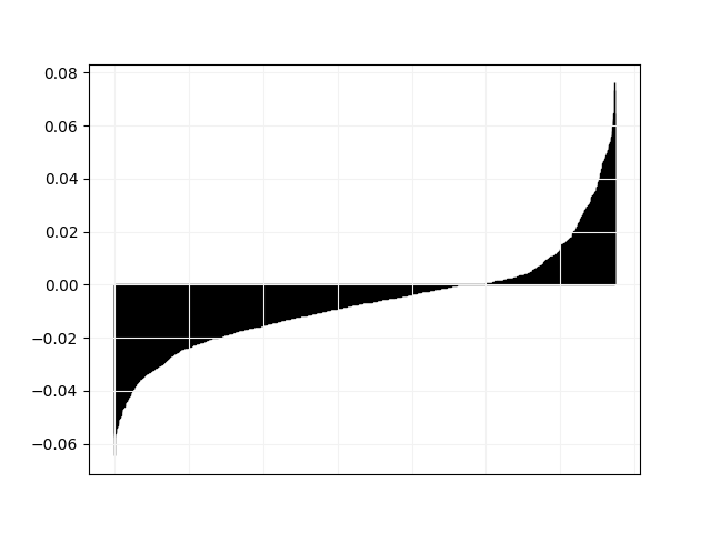
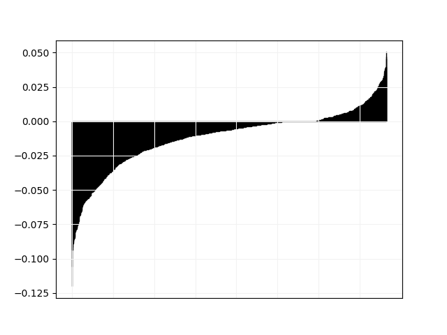
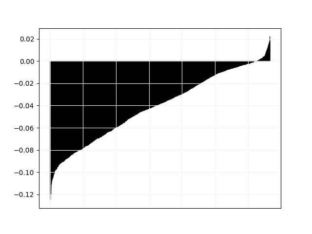
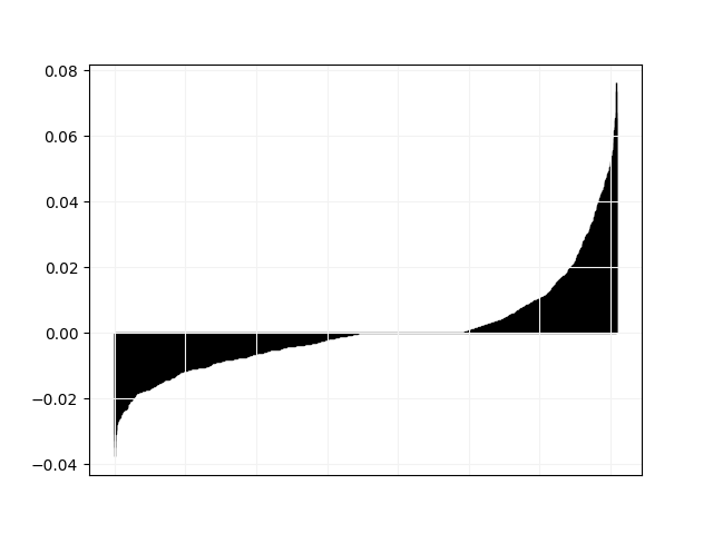
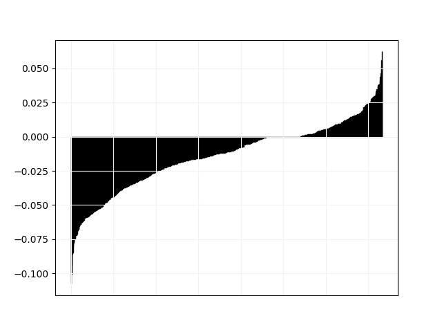
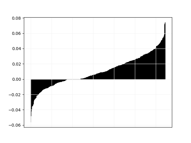
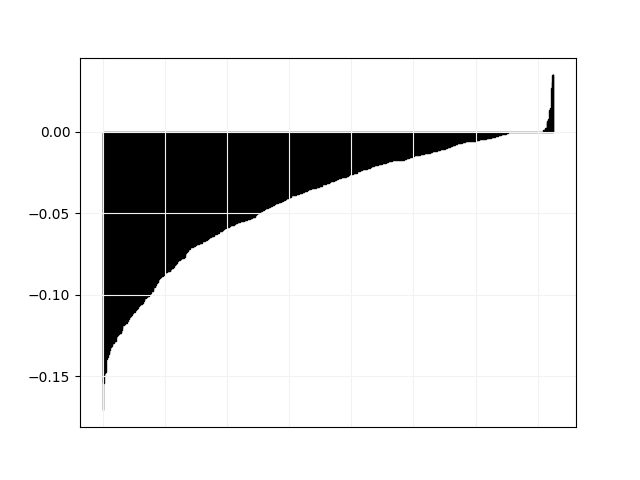
We plot in Fig. 3 and 4 pairwise comparisons of relative difference in objective value between Tempo and all other solvers. For every instance in the “hard” category, let be the objective value found by Tempo and the objective value found by the other solver, we plot the values of in non-decreasing order.
obj.png)