Analyzing Self-Stabilization of Synchronous Unison via Propositional Satisfiability

Abstract
Synchronous unison is a classical clock synchronization problem in distributed computing, and especially in self-stabilization. This paper explores the self-stabilization of a synchronous unison algorithm proposed by Arora et al. using a propositional satisfiability-based approach. We give a logical formulation of the algorithm. This formulation includes the uniqueness of clock values at each node, the updates of clocks based on the minimum clock value in the neighborhood, and the detection of convergence or divergence. To optimize the models, additional constraints are introduced to reduce redundant cases of initial configurations to be analyzed. Our approach not only verifies the algorithm’s behaviour but also offers insights into enhancing its robustness and applicability to broader distributed systems.
Keywords and phrases:
Self-stabilization, Synchronous Unison, SatisfiabilityCopyright and License:
2012 ACM Subject Classification:
Theory of computation Distributed algorithms ; Theory of computation Constraint and logic programming ; Theory of computation Logic and verificationSupplementary Material:
Software (Source Code and Benchmarks): https://github.com/asmakhoualdia98/SU_SAT_Exec [26]
archived at
Funding:
This work is supported by the project ANR-24-CE23-6126 (BforSAT), funded by the French National Research Agency. This work was also granted access to HPC resources of “Plateforme MatriCS” within University of Picardie Jules Verne, co-financed by the European Union with the European Regional Development Fund (FEDER) and the Hauts-De-France Regional Council among others.Editors:
Maria Garcia de la BandaSeries and Publisher:
1 Introduction
The notion of self-stabilization has been introduced in 1974 by Dijkstra [18] in the context of distributed systems. A distributed system is a set of computational entities, usually referred to as processes, that are both autonomous and interconnected. The goal of these processes is to cooperate to solve a task global to the system. An algorithm is said to be self-stabilizing if, regardless of the initial configuration of the system on which it is deployed, it guarantees to recover within finite time, and without external intervention, a so-called legitimate configuration from which the system specification is satisfied. Although the notion of failure is not explicit in the definition of self-stabilizing systems, the primary motivation of this approach is nevertheless fault tolerance. Indeed, after a finite number of transient failures111A transient fault occurs at an unpredictable time, but does not result in a permanent hardware damage. Moreover, as opposed to intermittent faults, the frequency of transient faults is considered to be low., the configuration of a distributed system may be arbitrary and thus no longer satisfy its specification. A self-stabilizing algorithm then guarantees that the system recovers from such faults within finite time.
Designing self-stabilizing algorithms may seem complex and subtle at first glance since processes only have a partial view of the global configuration of the system. Yet, many of these algorithms turn out to be surprisingly elegant and sometimes even simpler than their non-stabilizing counterparts. However, formally demonstrating the self-stabilization of an algorithm is often difficult and error-prone. This is mainly due to the combinatorial nature of the problem: convergence to a legitimate configuration must be demonstrated from every possible initial configuration. In the same spirit, our work aims at bringing formal reasoning techniques to the design and verification of self-stabilizing algorithms. In [19], the authors propose a formal approach based on propositional Satisfiability that is complementary to ours. First, as in the present paper, they aim at bringing formal reasoning techniques to the design and verification of self-stabilizing algorithms dedicated to synchronous distributed systems. Yet, their focus is on more severe failure patterns as they specifically consider both transient and Byzantine faults222A Byzantine fault refers to an arbitrary behavior of a node that may no longer follow its local algorithm.. However, their analysis is restricted to a fully connected network topology while our work addresses several classes of loosely connected topologies, including rings, chains and stars, where each node only accesses a very restrictive view of the system configuration.
With this in mind, we focus here on a simple problem: Synchronous Unison. We assume a synchronous system where processes are anonymous and whose topology is arbitrarily connected. Each process has a local clock whose integer values vary between 0 and , where is called the period. Starting from a configuration where each process’s clock has a set value in , the goal is to make the system converge to a configuration for which all clocks are identical while allowing increment actions (modulo ) at each step. Arora and al have proposed a simple solution to this problem [4]. The self-stabilization of their algorithm is demonstrated for all where is the diameter of the network [4, 3]. However, the tightness of this bound remains an open question. Actually, this question is partially answered in [3] where divergence configurations, i.e., configurations from which executions never stabilize, are exhibited for all even periods strictly smaller than the bound: the odd cases remaining unresolved to date.
We propose therefore to study how propositional satisfiability can help to address this question, and more generally how it can help to verify the self-stabilization of distributed algorithms. Indeed, Propositional Satisfiability (SAT) is a fundamental problem in logic and symbolic artificial intelligence, which consists in determining whether a given propositional formula in Conjunctive Normal Form (CNF) can be satisfied by an assignment of the variables. This problem, which was the first proven NP-complete [15], is attracting growing interest particularly due to the remarkable efficiency of modern SAT solvers in handling large instances despite its established difficulty. In addition to its key role in software verification, artificial intelligence, and cryptography, SAT lies at the intersection of several disciplines such as logic, graph theory, computer science, and artificial intelligence [6].
In this paper, we introduce a formal SAT-based approach to rigorously analyze the behavior of Arora and al’s synchronous unison algorithm [4]. Clock update rules are translated into logical constraints in CNF, allowing the use of SAT solvers to verify whether synchronization can be achieved. This methodology provides a systematic framework for studying the stabilization of the algorithm with different topologies and initial configurations, and with different periods. To optimize this analysis, specific techniques are applied to reduce redundancies among initial configurations, thereby accelerating model efficiency. Our approach, although focused on unison, provides formal guarantees regarding synchronization scenarios, while opening up optimization opportunities in more complex distributed algorithms.
The remainder of this paper is organized as follows. In Section 2, we present the synchronous unison algorithm and introduce propositional satisfiability. Section 3 is devoted to the formal modeling of the synchronous unison algorithm of Arora and al [4], where we detail the variables and notations, as well as the formulation of clock uniqueness, update, and detection of self-stabilization or its absence. This section also presents additional constraints that aim at accelerating the solving of the problem. Finally, Section 5 presents our experimental evaluation on different graph topologies. Finally, we conclude and discuss future work in Section 6.
2 Preliminaries
2.1 Synchronous Unison
We consider a distributed system of interconnected processes. The interconnection network is modeled by an undirected connected graph where is a set of vertices representing the processes and a set of edges representing bidirectional communication links between processes. The set of neighbors of a process will be denoted . Arora and al’s synchronous unison [4] is showcased in Algorithm 1. It is written in the atomic-state model, a locally shared memory model of computation where each node can directly read its state and those of its neighbors, but can only modify its own state.
Given an integer parameter common to all processes and called period, each process holds a single variable , which represents its clock. The state of a process is then its clock value. The configuration of the system is modeled by the vector associating each process with its state (its clock value). The set of possible configurations of the system is denoted by . The local algorithm of each process is made of a single rule of the form . The guard of the rule of is a predicate on the state of and those of its neighbors. The action part modifies the state of and, in this case, is thus an assignment of the clock of . In a given configuration, a process’s rule is said to be enabled if its guard is true. A configuration where no rule can be enabled is said to be terminal. The system is assumed to be synchronous: as long as the system is not in a terminal configuration, iterations are executed as follows. All processes whose rule can be enabled in the current configuration simultaneously execute their rule’s action, thus generating a new configuration , and so on. An execution of the algorithm is therefore a sequence of configurations such that for all , is obtained from in one synchronous iteration of the algorithm.
Inputs :
:
set of the neighbors of
:
a positive integer, the period
Variable:
, the clock of
Macro :
Rule :
The goal of the unison algorithm is to reach a configuration where all clocks are synchronized to an identical value. To this end, at each iteration, each process computes the minimum clock value in its closed neighborhood (i.e., ), and then modifies, if necessary, its clock to (see Algorithm 1). Gradually, the smallest values propagate in the network. This progress can only be disturbed by the appearance of 0 at some processes after their entire closed neighborhood has reached the maximum value . However, Arora et al. have shown that when is chosen sufficiently large (i.e., where is the diameter of ), these local resets cannot prevent the system from converging: regardless of the initial configuration , there necessarily exists a value such that all clocks have the same value in . Conversely, if is chosen too small, the execution may never converge. In this case, there exists a cycle between illegitimate configurations (i.e., configurations containing at least two different clock values).
Since the total number of possible configurations is , if the system is still in an illegitimate configuration after iterations, we can claim that the execution will never converge. Thus, it is sufficient to observe the first configurations of an execution in order to decide whether the execution converges or diverges. This number is very large and can lead to exponential modeling. We can therefore choose a more reasonable value for , even if it means not being able to decide in some cases.
Example 1.
Consider a process network G=( organized as a ring topology. Let and assume the initial configuration given in Figure 1. From , we obtain the execution prefix given in Table 1. The unison algorithm therefore reaches a legitimate configuration after 3 iterations.
| 2 | 4 | 0 | 1 | 4 | 4 | |
| 3 | 1 | 1 | 1 | 2 | 3 | |
| 2 | 2 | 2 | 2 | 2 | 3 | |
| 3 | 3 | 3 | 3 | 3 | 3 |
In the previous example, a legitimate configuration, where the clocks are synchronized, is eventually reached by the algorithm. However, when is chosen too small, there may exist configurations from which the clocks never synchronize. In this case, we will say that the system diverges. The convergence and divergence properties, formally defined below, highlight the importance of studying the behavior of distributed algorithms, and particularly synchronous unison, according to their parameter values (in this case, the period) [16, 20].
Definition 2 (Convergence).
Given a period , the synchronous unison algorithm executed on a graph of vertices converges when, for every initial configuration , the system reaches, within a finite number of iterations, a configuration where all clocks have the same value.
Definition 3 (Divergence).
The synchronous unison algorithm diverges for a given period in a graph of vertices when there exists an initial configuration from which the clocks never synchronize, i.e., there are infinitely many reached configurations containing at least two distinct clock values.
Example 4.
Consider a network of processes whose topology is a chain. Let and consider the initial configuration given in Figure 2. From this initial configuration, we obtain the execution prefix described in Table 2. Divergence is observable since the the configuration is identical to the initial one, , and both are illegitimate.
| 0 | 1 | 1 | |
| 1 | 1 | 0 | |
| 0 | 1 | 1 |
Our analysis will focus on the impact of graph topology and the period on synchronization. The following theorem provides an interesting general bound on the maximum number of iterations in a connected graph.
Theorem 5 ([3]).
The synchronous unison algorithm is self-stabilizing in every connected graph of diameter for . Its stabilization time, in this case, is at most iterations.
Finally, we stress out that we have carefully selected the synchronous unison as our case study with the goal of generalization to a broader class of distributed algorithms in mind. More precisely, we deal with the atomic-state model because it is the most commonly used model in the self-stabilizing literature and it is also close to other important models widely used in distributed computing, e.g., the local and congest models [29, 23]. The atomic-state model is a locally shared memory model so our approach can be straightforwardly generalized to handle algorithms working in systems where communication is made using communication registers. Furthermore, Synchronous Unison is representative of classical techniques used in self-stabilization. For example, the way clocks are updated follows the so-called “” rule that is used in many self-stabilizing algorithms such as the Breadth-First Search (BFS) spanning tree construction [22] and the asynchronous version of the unison [16]. More generally, we believe that our guidelines to model the transition relations are very general while issues related to symmetries that we tackle in the paper are also pretty usual in self-stabilization.
2.2 Propositional Satisfiability
Let be a set of propositional variables. A literal is a variable or its negation . A clause is a disjunction of literals. A formula in Conjunctive Normal Form (CNF) is a conjunction of clauses. An assignment {True, False} associates each variable with a Boolean value and can be represented as a set of literals. A literal is satisfied by an assignment if , otherwise it is falsified by . A clause is satisfied by an assignment if at least one of its literals is satisfied by , otherwise it is falsified by . A CNF formula is satisfiable if there exists an assignment that satisfies all its clauses, otherwise it is unsatisfiable. The satisfiability problem (SAT) thus consists in determining whether a given CNF formula is satisfiable. Although SAT is NP-complete[15], modern solvers based on the Conflict Driven Clause Learning (CDCL)[30] algorithm are efficient and can solve instances involving a large number of variables and clauses. Indeed, beyond clause learning and non-chronological backtracking, these solvers integrate powerful mechanisms such as lazy structures, dedicated branching heuristics, and restarts[10]. Moreover, the SAT problem is widely used to model and solve many complex combinatorial problems from various fields, notably in formal verification[14, 8], but also in cryptography, bioinformatics and planning, among many others [10].
Logic-based model checking has been a cornerstone in the formal verification of algorithms and systems. In particular, Bounded Model Checking (BMC) [7], which verifies whether a finite-state model satisfies a given specification within a bounded execution length, has gained significant traction over the past decade, especially when encoded as satisfiability (SAT) or satisfiability modulo theories (SMT) problems. Early efforts in the formal verification of distributed self-stabilizing algorithms were led by Lakhnech and Siegel [33, 27], who introduced theoretical frameworks for computer-aided verification, although no practical toolsets emerged from their work. Subsequent research explored symbolic BMC for distributed algorithms such as the work of Chen and Kulkarni who applied SMT-based BMC to assess the stabilization properties of distributed algorithms, particularly Dijkstra’s token ring, Ghosh’s Mutual Exclusion and a version tree-based mutual exclusion [13]. However, while SMT solvers offer expressive modeling capabilities, their higher-level abstraction can hinder fine-grained analysis and scalability. More recently, a SAT-based formal approach was proposed in [19] to detect Byzantine faults in synchronous systems with complete network topologies. This propositional encoding demonstrates the viability of SAT-based reasoning for distributed fault-tolerant systems and opens the door to more scalable and precise verification frameworks for self-stabilizing algorithms.
In the following sections, we thus focus on modeling the behavior of the synchronous unison algorithm, applied to an arbitrarily connected graph. The objective is to apply bounded model checking through SAT to characterize the conditions of convergence or divergence of the algorithm. This involves modeling the states of the processes using logical formulas, which must be expressed in such a way that they can be effectively solved by a SAT solver. Finally, we mention that previous literature introduces cardinality constraints having the form where each is a literal, and which can be efficiently encoded into CNF form [32].
3 Formal Modeling of Synchronous Unison
In this section, we focus on the formal modeling of the behavior of the synchronous unison of Arora et al. through propositional satisfiability. We begin by introducing the model variables. Then, we define the constraints that govern the execution of the algorithm. These constraints must faithfully represent the evolution of the system, and also allow us to detect its convergence or divergence. Furthermore, we will introduce specific constraints that allow us to optimize the model by eliminating redundant initial configurations.
3.1 Variables and Notations
We recall that the network is modeled by an undirected connected graph where is a set of vertices representing the processes and is a set of edges representing bidirectional communication links between pairs of processes. denotes the set of possible clock values, where is the period. We are interested in the first configurations of any execution of the algorithm on . The configurations will thus be indexed from 0 to and the set of indices will be denoted . To model the execution of the algorithm, it is also necessary to reason on the state of the process clocks in the different configurations. To do this, we introduce the clock variables , for all . Each variable will indicate whether the clock of process is equal to the value in configuration . This is sufficient to model execution and detect convergence. However, modeling divergence requires other variables, in particular to represent the presence of a cycle between illegitimate configurations during execution and to simplify the transformation of constraints into conjunctive normal form. The set of variables we will use is detailed below:
-
Clock variables: where . These variables are assigned to if process has clock value in configuration , otherwise.
-
Cycle variables: where . These variables are assigned to if the configuration and the initial configuration are identical, i.e., if the clock value of each process is identical in both configurations.
-
Clock-Similarity variables: where . These variables are assigned to True if process has the same clock value in configuration and the initial configuration.
3.2 Modeling Unison Execution
First, we focus on formalizing the constraints modeling a valid execution of synchronous unison. More specifically, we define clock uniqueness constraints as well as update rules ensuring the correct computation of clock values at each iteration.
3.2.1 Clock Uniqueness
To guarantee a valid execution of the algorithm, it is necessary to maintain the uniqueness of each process’s clock at each iteration. Specifically, it is necessary to ensure that each process has one and only one clock value at each configuration of the algorithm. This constraint can be modeled using the following cardinality constraint:
| (1) | |||
Note that this constraint can be easily rewritten in CNF form, using a pairwise encoding, without addition of auxiliary variables as shown below. The constraint (1a) ensures that a process cannot simultaneously hold two different clock values in a given configuration, while the constraint (1b) ensures that each process holds at least one valid clock value in each configuration. The number of clauses induced by these constraints is thus but more efficient encodings can be used if we allow the use of auxiliary variables [31].
| (1a) | |||
| (1b) | |||
3.2.2 Clock Update
The process clocks are updated, at each iteration, based on the clock values of their closed neighborhood. More precisely, each process computes the minimum values among its own clock value and those of its neighbors. This value will then be incremented by modulo . Finally, the obtained value is assigned to if . To simplify the notations, we denote the closed neighborhood of the process and its size. The clock update constraint is then modeled as follows:
| (3) |
Indeed, for each possible assignment of the clock values of the closed neighborhood of a process , we want to ensure that the minimum value incremented by 1 modulo , denoted , is propagated to the process at the following configuration, i.e., . This last implication perfectly highlights the clock update mechanism in the context of synchronous unison and is rewritten in conjunctive normal form in the constraint (3) by adding the necessary iterations on the possible assignments and the computation of the new value of the clock at the conjunction level. To provide a refined analysis of the encoding complexity, we denote the maximum degree of the graph. Thus, it is clear that the number of clauses is bounded by . Therefore, it seems that the complexity of our model is strongly correlated to the maximum degree in the graph and thus it is more suited to graphs in which this value remains relatively small. In particular, for ring or chain graphs, the complexity will be since, for these topologies, we have .
3.3 Modeling Convergence
Convergence occurs when the system has reached a legitimate configuration, where all clock values are identical. An algorithm is said to be convergent if, starting from any initial configuration, such a legitimate configuration is always reached within a finite number of iterations. To demonstrate this property, we will reason by contradiction by assuming that convergence is never reached from some initial configuration. In other words, there exists (at least) one initial configuration from which no legitimate configuration can be obtained. Since a legitimate configuration necessarily generates another legitimate configuration after an iteration of the algorithm, it suffices to show that the last configuration is illegitimate for some initial configuration. This property is thus translated by the following constraint:
| (4) |
Thus, it is clear that the CNF formula obtained thanks to the constraints (1), (3), and (4) is unsatisfiable if and only if the synchronous unison algorithm converges. Indeed, if is satisfiable, the provided model allows to exhibit an initial configuration deduced from the clock variables which are set to true for and , from which the algorithm does not converge. More specifically, in the valid execution of the unison algorithm from (ensured by the constraints (1) and (3)), we exhibit, at the level of the last configuration and for any possible clock value , a process whose clock does not hold the value in (ensured by constraint (4)). In terms of complexity, since constraint (4) requires only clauses, our model for convergence requires only variables with a number of clauses bounded by where is the maximum degree of the graph. We also note that the maximum clause size of the model is .
Additionally, we can notice that constraint (4) can be further imposed on any subset of configurations in as showcased in (5). Adding these redundant constraints does not alter the overall complexity of the model but may accelerate the detection of convergence. Specifically, these constraints can enable the solver to identify a valid configuration without requiring all necessary propagations to simulate the system execution until the final iteration from a given initial configuration. Consequently, if we consider the set , the model will ensure that the presence of a legitimate configuration is verified at each iteration of the algorithm whereas the set guarantees that this verification occurs every iterations, while necessarily including the initial configuration. We will thus refer to the following constraint as IC (for iterative convergence) and we denote the constraint with the corresponding set .
| (5) |
3.4 Modeling Divergence
Divergence implies the existence of two identical illegitimate configurations in the execution. Indeed, the set of legitimate configurations is trivially closed, and since the algorithm is synchronous and deterministic, such a cycle repeats itself infinitely. Let two configurations such that , where the clock values of the processes at are identical to those at . We will call such an occurrence a cycle at the level of configurations . To establish the divergence, we must therefore model the existence of a cycle at the level of two possible illegitimate configurations reached by the algorithm. To simplify the modeling, we consider the existence of a cycle with respect to the initial configuration, i.e., . Indeed, even if , it is always possible to reduce the analysis to the initial configuration by taking the configuration in as the initial configuration of the system (n.b., a self-stabilizing algorithm must converge from any initial configuration). Furthermore, to ensure that the cycle configurations are illegitimate, it is sufficient to check that the initial configuration is illegitimate. We recall that the variables where , defined previously, represent the existence of a cycle at configuration . Thus, the existence of a cycle between illegitimate configurations can be enforced by the following constraints:
| (6a) | ||||
| (6b) | ||||
Clearly, the constraint (6a) models the existence of a cycle where ; while the constraint (6b) guarantees that configuration 0, and therefore the configurations of the cycle, are illegitimate. To establish the semantic meaning of the cycle variables, it is necessary to guarantee that, if these variables are set to true, then there is a cycle , i.e., the clock values in configuration are identical to those in the initial configuration. In this context, the clock similarity variables where can play the intermediate role of guaranteeing the same clock value in configuration and the initial configuration. Thus, we add the following constraints:
| (7a) | ||||
| (7b) | ||||
The constraint (7a) thus ensures that the corresponding configuration has the same clock values as configuration or, more formally, that . The normal form presented in the constraint (7a) can be simply obtained by the clausal rewriting of the implication as well as the distributivity of disjunctions over logical conjunctions. The constraint (7b) is necessary to establish the semantic meaning of the variables which are set to when the process has the same clock value at configurations and . More formally, we have and its normal form presented in the constraint (7b) can also be deduced by rewriting the implication and applying the distributivity of disjunction.
It is clear that the CNF formula obtained by the constraints (1), (3), (6) and (7) is satisfiable if and only if the unison algorithm diverges on the given input network with period . Indeed, a model of allows to exhibit an initial configuration from which a valid execution of the synchronous unison generates a cycle of illegitimate configurations, given by a cycle variable assigned to at the level of the clausal constraint (6a). Moreover, in terms of encoding complexity for divergence, it is clear that the constraints (6) and (7) introduce a bounded number of clauses in and, consequently, the model has a complexity similar to the convergence case, mainly governed by the constraint (3), i.e., in where is the maximum degree of the graph. However, the model requires a larger number of variables, but which remains in .
3.5 Elimination of Initial Configurations
In this section, we aim at reducing the number of initial configurations to be processed by removing redundant configurations. In other words, the goal is to eliminate configurations for which the algorithm’s behavior is identical to that of other configurations we already consider in the analysis. This approach optimizes the algorithm’s execution by avoiding processing situations that, although different in their representation, do not lead to different results.
3.5.1 Lexicographic Order
Within the framework of the unison algorithm, the evolution of process clock values depends exclusively on their local neighborhood and, more specifically, on their closed neighborhood. In particular, two processes with the same set of neighbors in the studied topology evolve identically, up to any permutation of their initial clock values. This observation makes it possible to exploit a structural symmetry to reduce the space of configurations to be considered by establishing a specific lexicographic order on the initial clock values for processes with identical neighborhoods in the topology. To take advantage of this symmetry and avoid examining multiple equivalent configurations, we introduce constraints imposing a lexicographic order on the configurations. More precisely, only the minimal configurations according to this order are considered, which eliminates redundant configurations and reduces the search space. In our case, we will introduce constraints prohibiting lexicographically larger configurations on local neighborhoods identical to those selected. This constraint, which we will denote LO, can be formulated as follows:
| (8) |
Thus, if two processes such that have an identical neighborhood, the constraint (8) guarantees that cannot take an initial clock value smaller than that of . This constraint introduces a number of clauses bounded in and can only be applied in topologies where some processes have an identical neighborhood, such as in the star topology, where a central process (hub) is connected to several peripheral processes (see Figure 5), or in complete graphs.
3.5.2 Rotation Elimination
As previously discussed, when a transformation of an initial configuration does not modify the overall behavior of the algorithm, it is possible to eliminate redundant configurations to optimize the search and analysis of relevant cases. A particularly interesting case concerns graphs, such as rings, where the same configuration can be expressed in several equivalent forms via a simple rotation of the process indices. In these structures, any initial configuration can be transformed into another configuration by uniformly shifting the clock values. Since the rotation does not modify either the neighbor relationships or the algorithm dynamics, the study can be restricted to a representative subset of possible configurations.
To enforce this restriction, a constraint can be introduced guaranteeing that, among all equivalent configurations, only those where a specific process has the lowest clock value are considered. In particular, in a ring graph of processes, we consider a configuration where the first process has the lowest clock value among the clock values of the other processes in the same configuration. Since the rotation, whether in the direct or indirect direction, preserves the same behavior of the synchronous unison algorithm, we can eliminate any other initial configuration that is an image of this configuration in order to avoid the analysis of redundant cases, as proven in Proposition 6, with denoting the clock value of in the configuration . This constraint, which we will denote RE, can therefore be expressed as follows on any ring topology:
| (9) |
Proposition 6.
Let be a ring graph composed of processes and a period. Let . Then, for any initial configuration , there exists a configuration from which a synchronous unison execution produces the same convergence or divergence behavior.
Proof.
Without loss of generality, we assume that . Let and . We define the configuration such that:
Clearly, is obtained by a rotation of that brings the smallest value back to process 0. Therefore, has the same behavior as , up to a rotation. Indeed, following an execution of the synchronous unison algorithm in a ring graph, the relations between neighbors are preserved under rotation and each process applies exactly the same evolution rules as its representative in the original configuration. Moreover, since , there is no process such that and, therefore, belongs to the kernel .
The constraint (9) introduces a number of clauses bounded in and can be applied to graphs whose topology allows for specific rotations while preserving neighbor relationships such as rings, or star topologies by applying the constraint only to the peripheral nodes.
4 Experimental Evaluation
4.1 Experimental Protocol
We consider the following classical network topologies: chains, rings, and stars (see Figures 1, 2, and 5 respectively) [34]. The properties of the considered graphs and periods are summarized in Table 3. We encoded our models in Python using the PySAT library [25] 333Our code and benchmark are available in the following GitHub repository and solved these instances using the state-of-the-art solvers Cadical [9] and MapleSAT [28] 444For lack of space, we present the results with Cadical and we provide a comparison on the initial models of convergence and divergence in the appendix (refer to Tables 10, 9 and 8). Tests were performed on a machine equipped with an Intel Core i7 processor clocked at 3.80 GHz, running under Ubuntu 22.04. A timeout of 7200 seconds was set for each instance. We have generated the instances associated with all our models, totaling 4968 instances. For each type of topology among rings and chains, we took graph sizes ranging from to nodes, and we varied the period from to . For the star topology, we took graph sizes ranging from to nodes, and we varied the period from to . In particular, we generated 756 instances (342 for chains and rings and 72 for stars) for the initial model of convergence () which is described by the constraints (1), (3) and (4). Similarly we generated the same number of instances for the divergence model () described through the constraints (1), (3), (6) and (7).
| Topology | n | m | ||
|---|---|---|---|---|
| Chain | {2,…,20} | 2 | ||
| Ring | {2,…,20} | 2 | ||
| Star | {2,…,10} | 2 |
Furthermore, for topologies where initial configuration elimination constraints can be applied, we also generate the corresponding instances. Thus, we generated 828 instances of convergence and divergence for ring and star topologies with the rotation elimination (RE) constraint. For the lexicographic order (LO) constraint, we generated 144 instances of convergence and divergence for the star topology. Moreover, we generated 756 instances of convergence for ring, chain, and star topologies for each constraint and , added on top of the initial models. 414 instances of convergence were generated for ring and star topologies with each combinations and . Finally, we generated 72 instances of convergence for star topology for each combination and . The number of allowed configurations is set to for all topologies where is the diameter of the considered graph. We also note that the Cardinality Network encoding [5] was used to rewrite constraint (1) in CNF form.
4.2 Analysis of Convergence and Divergence
| 20 | ✓ | ✓ | ✓ | ✓ | ✓ | ✓ | ✓ | ✓ | ✓ | ✓ | ✓ | ✓ | ✓ | ✓ | ✓ | ✓ | ✓ | ✓ |
|---|---|---|---|---|---|---|---|---|---|---|---|---|---|---|---|---|---|---|
| 19 | ✓ | ✓ | ✓ | ✓ | ✓ | ✓ | ✓ | ✓ | ✓ | ✓ | ✓ | ✓ | ✓ | ✓ | ✓ | ✓ | ✓ | - |
| 18 | ✓ | ✓ | ✓ | ✓ | ✓ | ✓ | ✓ | ✓ | ✓ | ✓ | ✓ | ✓ | ✓ | ✓ | ✓ | - | - | |
| 17 | ✓ | ✓ | ✓ | ✓ | ✓ | ✓ | ✓ | ✓ | ✓ | ✓ | ✓ | ✓ | ✓ | ✓ | ✓ | ✓ | ✓ | |
| 16 | ✓ | ✓ | ✓ | ✓ | ✓ | ✓ | ✓ | ✓ | ✓ | ✓ | ✓ | ✓ | ✓ | ✓ | ✓ | |||
| 15 | ✓ | ✓ | ✓ | ✓ | ✓ | ✓ | ✓ | ✓ | ✓ | ✓ | ✓ | ✓ | ✓ | ✓ | ✓ | X | X | |
| 14 | ✓ | ✓ | ✓ | ✓ | ✓ | ✓ | ✓ | ✓ | ✓ | ✓ | ✓ | ✓ | ✓ | |||||
| 13 | ✓ | ✓ | ✓ | ✓ | ✓ | ✓ | ✓ | ✓ | ✓ | ✓ | ✓ | ✓ | ✓ | X | X | X | ||
| 12 | ✓ | ✓ | ✓ | ✓ | ✓ | ✓ | ✓ | ✓ | ✓ | ✓ | ✓ | |||||||
| 11 | ✓ | ✓ | ✓ | ✓ | ✓ | ✓ | ✓ | ✓ | ✓ | ✓ | ✓ | X | X | X | X | X | X | |
| 10 | ✓ | ✓ | ✓ | ✓ | ✓ | ✓ | ✓ | ✓ | ✓ | |||||||||
| 9 | ✓ | ✓ | ✓ | ✓ | ✓ | ✓ | ✓ | ✓ | ✓ | X | X | X | X | X | X | X | X | X |
| 8 | ✓ | ✓ | ✓ | ✓ | ✓ | ✓ | ✓ | |||||||||||
| 7 | ✓ | ✓ | ✓ | ✓ | ✓ | ✓ | ✓ | X | X | X | X | X | X | X | X | X | ||
| 6 | ✓ | ✓ | ✓ | ✓ | ✓ | |||||||||||||
| 5 | ✓ | ✓ | ✓ | ✓ | ✓ | X | X | X | X | X | X | X | X | X | X | |||
| 4 | ✓ | ✓ | ✓ | |||||||||||||||
| 3 | ✓ | ✓ | ✓ | ✓ | X | X | X | X | X | X | ||||||||
| 2 | ✓ | |||||||||||||||||
| 3 | 4 | 5 | 6 | 7 | 8 | 9 | 10 | 11 | 12 | 13 | 14 | 15 | 16 | 17 | 18 | 19 | 20 |
| 20 | ✓ | ✓ | ✓ | ✓ | ✓ | ✓ | ✓ | ✓ | ✓ | |||||||||
|---|---|---|---|---|---|---|---|---|---|---|---|---|---|---|---|---|---|---|
| 19 | ✓ | ✓ | ✓ | ✓ | ✓ | ✓ | ✓ | ✓ | ✓ | X | X | X | ||||||
| 18 | ✓ | ✓ | ✓ | ✓ | ✓ | ✓ | ✓ | ✓ | ||||||||||
| 17 | ✓ | ✓ | ✓ | ✓ | ✓ | ✓ | ✓ | ✓ | X | X | X | X | X | X | ||||
| 16 | ✓ | ✓ | ✓ | ✓ | ✓ | ✓ | ✓ | |||||||||||
| 15 | ✓ | ✓ | ✓ | ✓ | ✓ | ✓ | ✓ | X | X | X | X | X | X | X | X | |||
| 14 | ✓ | ✓ | ✓ | ✓ | ✓ | ✓ | ||||||||||||
| 13 | ✓ | ✓ | ✓ | ✓ | ✓ | ✓ | X | X | X | X | X | X | X | X | X | X | X | |
| 12 | ✓ | ✓ | ✓ | ✓ | ✓ | |||||||||||||
| 11 | ✓ | ✓ | ✓ | ✓ | ✓ | X | X | X | X | X | X | X | X | X | X | X | X | X |
| 10 | ✓ | ✓ | ✓ | ✓ | ||||||||||||||
| 9 | ✓ | ✓ | ✓ | ✓ | X | X | X | X | X | X | X | X | X | X | X | X | X | X |
| 8 | ✓ | ✓ | ✓ | |||||||||||||||
| 7 | ✓ | ✓ | ✓ | X | X | X | X | X | X | X | X | X | X | X | X | X | X | X |
| 6 | ✓ | ✓ | ||||||||||||||||
| 5 | ✓ | ✓ | X | X | X | X | X | X | X | X | X | X | X | X | X | X | X | X |
| 4 | ✓ | |||||||||||||||||
| 3 | ✓ | ✓ | ✓ | ✓ | ✓ | ✓ | ✓ | ✓ | ✓ | ✓ | ✓ | ✓ | ✓ | ✓ | ✓ | ✓ | ✓ | ✓ |
| 2 | ||||||||||||||||||
| 3 | 4 | 5 | 6 | 7 | 8 | 9 | 10 | 11 | 12 | 13 | 14 | 15 | 16 | 17 | 18 | 19 | 20 |
The results presented in Figures 3(a), 3(b), and 4 illustrate the behavior of the synchronous unison in terms of convergence and divergence on the different topologies (rings, chains, and stars) as a function of size and period . For the studied graph topologies, we clearly notice that the results are coherent with Theorem 5 when . revealing a convergence for the corresponding instances. Notably, the generated results demonstrate unison behavior on many instances across different topologies for which it was previously unknown. In particular, we were able to detect the convergence of the algorithm for the three topologies for values of . However, some instances remain unsolved, most likely due to the chosen upper limit on the number of allowed steps (i.e., ). It is also interesting to note that our results show that the bound proposed in the theorem 5 is tight in the case of stars. Indeed, this theorem states that convergence is guaranteed in stars (of diameter 2) from a period greater than or equal to 3 (). Our results exhibit a case of divergence with in star graphs as shown in Figure 4, independently of their sizes. Thus, the synchronous unison algorithm converges in a star if and only if . We demonstrate this property in following proposition.
Proposition 7.
The synchronous unison algorithm diverges for any star graph, regardless of its number of nodes , with period .
Proof.
We can always exhibit an initial configuration that causes the synchronous unison to diverge. Such a configuration is illustrated in Figure 1, where the initial clock value of the central node is set to 1, while the clock values of the peripheral nodes take at least two distinct initial values. The prefix of execution until a cycle is detected is represented in Table 4 and therefore the algorithm diverges on star graphs when .
| 10 | ✓ | ✓ | ✓ | ✓ | ✓ | - | - | - |
|---|---|---|---|---|---|---|---|---|
| 9 | ✓ | ✓ | ✓ | ✓ | ✓ | - | - | - |
| 8 | ✓ | ✓ | ✓ | ✓ | ✓ | - | - | - |
| 7 | ✓ | ✓ | ✓ | ✓ | ✓ | ✓ | - | - |
| 6 | ✓ | ✓ | ✓ | ✓ | ✓ | ✓ | - | - |
| 5 | ✓ | ✓ | ✓ | ✓ | ✓ | ✓ | ✓ | - |
| 4 | ✓ | ✓ | ✓ | ✓ | ✓ | ✓ | ✓ | ✓ |
| 3 | ✓ | ✓ | ✓ | ✓ | ✓ | ✓ | ✓ | ✓ |
| 2 | ||||||||
| 3 | 4 | 5 | 6 | 7 | 8 | 9 | 10 |
| … | … | ||||||
| 1 | 0 | … | 0 | 1 | … | 1 | |
| 0 | 1 | … | 1 | 0 | … | 0 | |
| 1 | 0 | … | 0 | 1 | … | 1 |
4.3 Performance Analysis


| CONVERGENCE | DIVERGENCE | |||||||
|---|---|---|---|---|---|---|---|---|
| INICNV | RE | ICP | ICX | ER + ICP | ER + ICX | INIDIV | RE | |
| 3 | 0.025 | 0.023 | 0.025 | 0.022 | 0.025 | 0.024 | 0.05 | 0.02 |
| 4 | 0.69 | 0.48 | 0.66 | 0.62 | 0.42 | 0.29 | 1.48 | 0.33 |
| 5 | 1.97 | 1.59 | 1.85 | 1.88 | 1.73 | 1.79 | 2.33 | 0.48 |
| 6 | 7.34 | 1.13 | 6.90 | 6.93 | 7.21 | 6.74 | 9.46 | 2.71 |
| 7 | 11.58 | 2.07 | 11.75 | 10.87 | 11.08 | 11.59 | 15.00 | 4.10 |
| 8 | 36.25 | 29.72 | 31.62 | 31.38 | 26.57 | 25.66 | 48.89 | 12.15 |
| 9 | 55.56 | 47.01 | 49.06 | 46.70 | 46.40 | 40.84 | 68.76 | 18.87 |
| 10 | 109.10 | 111.82 | 100.48 | 105.55 | 92.27 | 88.04 | 141.30 | 54.98 |
| 11 | 187.26 | 161.45 | 151.87 | 151.41 | 149.89 | 135.45 | 231.78 | 82.91 |
| 12 | 331.62 | 288.23 | 312.34 | 275.70 | 273.22 | 263.15 | 427.35 | 148.67 |
| 13 | 420.22 | 384.39 | 387.10 | 348.26 | 341.03 | 360.64 | 503.95 | 258.33 |
| 14 | 658.15 | 629.41 | 573.85 | 583.77 | 749.07 | 494.72 | 844.47 | 417.39 |
| 15 | 858.95 | 836.12 | 794.91 | 871.29 | 1045.89 | 743.99 | 1172.70 | 532.67 |
| 16 | 1500.84 | 1324.06 | 1279.63 | 1292.98 | 1216.69 | 1250.76 | 852.05 [16] | 779.99 |
| 17 | 819.73 [16] | 1654.83 | 1757.84 | 1446,94 | 1506.43 [18] | 1400.94 | 1196.05 [16] | 996.15 |
| 18 | 73.47 [15] | 518.55 [16] | 79.97 [15] | 58.06 [15] | 61.10[15] | 504.26 [16] | 560.75 [15] | 846.22 [17] |
| 19 | 44.35 [15] | 116.42 [15] | 77.05 [15] | 97.72 [15] | 82.12[15] | 55.32[15] | 1164.60 [14] | 862.39 [17] |
| 20 | 166.89 [17] | 310.59 [17] | 111.46 [17] | 125.39 [17] | 283.68[17] | 449.56 [17] | 502.73 [13] | 995.53 [17] |
| CONVERGENCE | DIVERGENCE | |||||||||||
|---|---|---|---|---|---|---|---|---|---|---|---|---|
| INICNV | RE | LO | ICP | ICX | RE + ICP | RE + ICX | LO + ICP | LO + ICX | INIDIV | RE | LO | |
| 3 | 0.007 | 0.006 | 0.002 | 0.004 | 0.004 | 0.004 | 0.003 | 0.004 | 0.004 | 0.01 | 0.01 | 0.02 |
| 4 | 0.04 | 0.03 | 0.02 | 0.045 | 0.04 | 0.034 | 0.03 | 0.02 | 0.02 | 0.09 | 0.04 | 0.05 |
| 5 | 1.00 | 0.86 | 0.31 | 0.83 | 0.95 | 0.94 | 0.59 | 0.31 | 0.20 | 0.90 | 0.49 | 0.33 |
| 6 | 27.38 | 19.72 | 4.19 | 25.06 | 28.37 | 17.41 | 13.75 | 7.10 | 7.14 | 6.97 | 4.48 | 3.43 |
| 7 | 862.27 | 746.24 | 97.84 | 868.23 | 828.41 | 634.05 | 730.64 | 102.46 | 696.16 | 76.61 | 55.18 | 28.88 |
| 8 | 553.70 [6] | 936.88 [7] | 32.60 [6] | 652.89 [6] | 547.38 [6] | 473.89 [6] | 171.55 [6] | 24.19 [6] | 93.25 [6] | 146.91[6] | 96.12 [6] | 23.75 [6] |
| 9 | 119.25 [4] | 542.24 [5] | 43.60 [5] | 212.08[4] | 139.36 [4] | 185.13 [4] | 184.93 [4] | 42.01 [5] | 33.88 [5] | 166.68[5] | 67.94 [5] | 16,79 [5] |
| 10 | 67.71 [3] | 487.43 [4] | 40.21 [4] | 86.60 [3] | 75.33 [3] | 22.51[3] | 598.80 [4] | 39.14 [4] | 68.56 [4] | 76.16[3] | 432.92 [4] | 52.76 [4] |
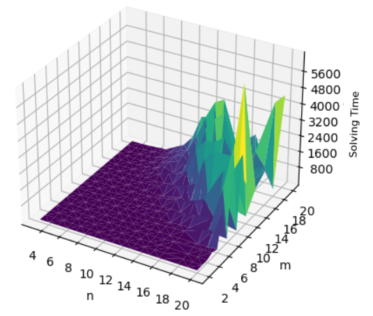
In this section, we analyze the performance of the models on the different topologies in terms of number of solved instances and average solving time per graph size. The results obtained for ring and star graphs are presented respectively in Tables 5 and 7, with respect to the graph sizes, the analyzed property, and the considered model. Due to the lack of space, the results obtained for chain graphs have been moved to the appendix (refer to Table 6). The results indicate that the initial model manages to solve most of the instances but it clearly encounters increasing difficulties with increasing graph sizes, particularly for the star and ring topologies. It thus manages to solve 329 (resp. 321) instances out of 342 for the convergence (resp. divergence) check on rings and 58 (resp. 59) instances out of 72 for the convergence (resp. divergence) check on stars. For chains, all instances were solved for convergence with the initial model whereas 328 out of 342 were solved for divergence. This behavior is not surprising especially for stars, since the star topology has a maximum degree , which leads to a combinatorial explosion in the number of clauses generated by the constraint (3). Indeed, it increases with a complexity of the order , which explains the model’s difficulty in handling larger instances. Figures 6 (resp. 7) illustrates the evolution of the solving time of instances generated for convergence (resp. divergence) verification for the initial model, as a function of graph size and period , for ring, chain and star topologies. These curves highlight a progressive increase in resolution time as these two parameters increase. We observe in particular that, in the case of star graphs, this increase is much more pronounced for relatively smaller values of and compared to the other topologies. This trend, which remains similar both for convergence and divergence corroborates our previous observations and confirms the increased complexity of the model for topologies whose maximal node degree is high.
Next, we focus on comparing the initial convergence model (INICNV) with its counterparts augmented with the constraint, specifically and , across ring, star, and chain topologies. In the ring topology (Table 5), consistently outperforms and INICNV in larger instances, achieving the lowest solving times (-10,21% w.r.t INICNV) and highest number of solved instances (+3 w.r.t INICNV). For the star topology (Table 6), although convergence times are higher overall, still shows better performance than in mid-sized to larger instances. In the chain topology (Table 7), also stands out as it achieves the lowest convergence times (-5,97% w.r.t ). Overall, added on top of the initial model emerges as the most effective in convergence detection, balancing low solving times with a higher number of solved instances.
Finally, we study the formulations augmented by the constraints eliminating the initial configurations. As illustrated in Tables 5 and 6, the comparison with the initial models highlights the relevance of introducing these constraints, particularly for the divergence analysis. The results show a significant reduction in solving time for ring and star topologies thanks to rotation elimination (RE) and lexicographic order (LO), particularly when they are combined with Iterative Convergence (IC) constraints. More specifically, for ring graphs, the ER and ICX combination model achieves the best overall performance, with an average solving time of 324.10s for convergence. For divergence, RE achieves better performance with respect to the initial model with an average solving time of 596.52s, across all graph sizes tested. Compared to the initial model, ER + ICX thus reduces the total solving time by 10,5% with a higher number of solved instances (+4 w.r.t INICNV) for convergence and ER reduces it by 55,14% for divergence while solving 15 additional instance with respect to INIDIV. These results demonstrate the positive impact of the symmetry-breaking constraints on the analysis of synchronous unison behavior. The star graph reveals a better dynamic with LO which demonstrates a significant improvement in the divergence time with an average of 15,80s, a reduction of 81.5% compared to the initial model (59,29s) with a higher number of solved instances (+1 w.r.t INIDIV). On the other hand, LO + ICP presents a significant reduction in solving time for convergence with a total of 215,23s, a reduction of 90,71% compared to the initial model (1631,35s) and a higher number of solved instances (+2 w.r.t INICNV). These observations are also confirmed by Table 6 and highlight the relevance of this optimization in structures where interactions are highly centralized around a central node.
5 Conclusion
In this paper, we presented a formal approach based on propositional satisfiability to analyze the behavior of the self-stabilizing synchronous unison algorithm proposed by Arora et al. [4]. Specifically, we focused on detecting cases where this algorithm converges or diverges. By representing the problem states and its execution as logical constraints, we showed how SAT solvers can be used to prove the self-stabilization of a distributed system or, conversely, to produce a counterexample proving its divergence. This framework allowed us to rigorously study the self-stabilization of the algorithm in various topologies such as chains, rings and stars, while taking into account different periods. Furthermore, we optimized the analysis by proposing specific constraints to eliminate redundant initial configurations, which accelerated model evaluation and ensured more efficient results. Our models also exhibited specific behaviors, notably divergence in the case of stars when .
Several avenues of research remain open. First, extending our analysis to other types of graphs, such as grids, tori, or binary trees, would allow for a more comprehensive and detailed examination of the impact of the topology on the algorithm’s self-stabilization. It could be also relevant to consider refining the choice of the maximum number of allowed configurations relative to the topology studied. Another interesting perspective involves considering symmetries for the detection of divergent cycles. These perspectives pave the way for a better understanding of synchronization dynamics in complex distributed systems and for the development of new, more efficient and optimized methods to address a wider range of application cases. Our work could thus facilitate not only the analysis of synchronous unison, but more generally that of self-stabilizing algorithms in broader and more diverse contexts including the asynchronous case [16, 17], variants of self-stabilization [11, 12], reactive tasks [1, 24] and the possibility of topological change [21, 2].
References
- [1] Karine Altisen, Stéphane Devismes, and Anaïs Durand. Concurrency in snap-stabilizing local resource allocation. Journal Of Parallel and Distributed Computing, 102:42–56, 2017. doi:10.1016/J.JPDC.2016.11.004.
- [2] Karine Altisen, Stéphane Devismes, Anaïs Durand, Colette Johnen, and Franck Petit. Self-stabilizing systems in spite of high dynamics. Theor. Comput. Sci., 964:113966, 2023. doi:10.1016/J.TCS.2023.113966.
- [3] Karine Altisen, Stéphane Devismes, Swan Dubois, and Franck Petit. Introduction to Distributed Self-Stabilizing Algorithms. Synthesis Lectures on Distributed Computing Theory. Morgan & Claypool, 2019.
- [4] Anish Arora, Shlomi Dolev, and Mohamed G. Gouda. Maintaining digital clocks in step. Parallel Processing Letters, 1:11–18, 1991. doi:10.1007/bfb0022438.
- [5] Roberto Asín, Robert Nieuwenhuis, Albert Oliveras, and Enric Rodríguez-Carbonell. Cardinality networks and their applications. In Oliver Kullmann, editor, Theory and Applications of Satisfiability Testing – SAT 2009, 12th International Conference, SAT 2009, Swansea, UK, June 30 – July 3, 2009. Proceedings, volume 5584 of Lecture Notes in Computer Science, pages 167–180. Springer, 2009. doi:10.1007/978-3-642-02777-2_18.
- [6] Armin Biere. Handbook of satisfiability. In Frontiers in Artificial Intelligence and Applications, pages 75–98. IOS Press, 2009. doi:10.3233/978-1-58603-929-5-75.
- [7] Armin Biere. Bounded model checking. In Armin Biere, Marijn Heule, Hans van Maaren, and Toby Walsh, editors, Handbook of Satisfiability – Second Edition, volume 336 of Frontiers in Artificial Intelligence and Applications, pages 739–764. IOS Press, 2021. doi:10.3233/FAIA201002.
- [8] Armin Biere et al. Symbolic model checking without bdds. In Proceedings of the International Conference on Tools and Algorithms for the Construction and Analysis of Systems (TACAS), pages 193–207, 1999.
- [9] Armin Biere, Tobias Faller, Katalin Fazekas, Mathias Fleury, Nils Froleyks, and Florian Pollitt. Cadical 2.0. In Arie Gurfinkel and Vijay Ganesh, editors, Computer Aided Verification – 36th International Conference, CAV 2024, Montreal, QC, Canada, July 24-27, 2024, Proceedings, Part I, volume 14681 of Lecture Notes in Computer Science, pages 133–152. Springer, 2024. doi:10.1007/978-3-031-65627-9_7.
- [10] Armin Biere, Marijn Heule, and Hans van Maaren. Handbook of Satisfiability: Second Edition. Frontiers in Artificial Intelligence and Applications. IOS Press, 2021. URL: https://books.google.fr/books?id=dUAvEAAAQBAJ.
- [11] James E. Burns, Mohamed G. Gouda, and Raymond E. Miller. Stabilization and pseudo-stabilization. Distributed Computing, 7(1):35–42, 1993. doi:10.1007/BF02278854.
- [12] Fabienne Carrier, Ajoy Kumar Datta, Stéphane Devismes, Lawrence L. Larmore, and Yvan Rivierre. Self-stabilizing (f, g)-alliances with safe convergence. J. Parallel Distributed Comput., 81-82:11–23, 2015. doi:10.1016/J.JPDC.2015.02.001.
- [13] Jingshu Chen and Sandeep S. Kulkarni. Smt-based model checking for stabilizing programs. In Davide Frey, Michel Raynal, Saswati Sarkar, Rudrapatna K. Shyamasundar, and Prasun Sinha, editors, Distributed Computing and Networking, 14th International Conference, ICDCN 2013, Mumbai, India, January 3-6, 2013. Proceedings, volume 7730 of Lecture Notes in Computer Science, pages 393–407. Springer, 2013. doi:10.1007/978-3-642-35668-1_27.
- [14] Edmund M. Clarke and E. Allen Emerson. Design and synthesis of synchronization skeletons using branching-time temporal logic. In Dexter Kozen, editor, Logics of Programs, Workshop, Yorktown Heights, New York, USA, May 1981, volume 131 of Lecture Notes in Computer Science, pages 52–71. Springer, 1981. doi:10.1007/BFB0025774.
- [15] Stephen A. Cook. The complexity of theorem-proving procedures. Proceedings of the Third Annual ACM Symposium on Theory of Computing (STOC), pages 151–158, 1971. doi:10.1145/800157.805047.
- [16] J.-M. Couvreur, N. Francez, and M. G. Gouda. Asynchronous unison (extended abstract). In 12th International Conference on Distributed Computing Systems, (ICDCS’92), pages 486–493. IEEE Computer Society, 1992. doi:10.1109/ICDCS.1992.235005.
- [17] Stéphane Devismes, David Ilcinkas, Colette Johnen, and Frédéric Mazoit. Being efficient in time, space, and workload: a self-stabilizing unison and its consequences. In Olaf Beyersdorff, Michal Pilipczuk, Elaine Pimentel, and Kim Thang Nguyen, editors, 42nd International Symposium on Theoretical Aspects of Computer Science, STACS 2025, March 4-7, 2025, Jena, Germany, volume 327 of LIPIcs, pages 30:1–30:18. Schloss Dagstuhl – Leibniz-Zentrum für Informatik, 2025. doi:10.4230/LIPICS.STACS.2025.30.
- [18] Edsger W. Dijkstra. Self-stabilizing systems in spite of distributed control. Commun. ACM, 17(11):643–644, 1974. doi:10.1145/361179.361202.
- [19] Danny Dolev, Keijo Heljanko, Matti Järvisalo, Janne H. Korhonen, Christoph Lenzen, Joel Rybicki, Jukka Suomela, and Siert Wieringa. Synchronous counting and computational algorithm design. J. Comput. Syst. Sci., 82(2):310–332, 2016. doi:10.1016/J.JCSS.2015.09.002.
- [20] Danny Dolev and Dahlia Malkhi. Consensus: Perspectives and challenges. In Proceedings of the Tenth International Workshop on Distributed Algorithms (WDAG), pages 1–12, 1995. doi:10.1007/3-540-60220-8_1.
- [21] Shlomi Dolev and Ted Herman. Superstabilizing protocols for dynamic distributed systems. Chicago Journal of Theoretical Computer Science, 1995.
- [22] Shlomi Dolev, Amos Israeli, and Shlomo Moran. Self-stabilization of dynamic systems assuming only read/write atomicity. Distrib. Comput., 7(1):3–16, November 1993. doi:10.1007/BF02278851.
- [23] Stéphane Grumbach and Zhilin Wu. Logical locality entails frugal distributed computation over graphs (extended abstract). In Christophe Paul and Michel Habib, editors, WG, volume 5911 of Lecture Notes in Computer Science, pages 154–165, 2009. doi:10.1007/978-3-642-11409-0_14.
- [24] Rachid Hadid. A stabilising optimal k-out-of- resources allocation algorithm. Int. J. Knowl. Eng. Data Min., 5(3):173–194, 2018. doi:10.1504/IJKEDM.2018.10014813.
- [25] Alexey Ignatiev, António Morgado, and João Marques-Silva. Pysat: A python toolkit for prototyping with SAT oracles. In Olaf Beyersdorff and Christoph M. Wintersteiger, editors, Theory and Applications of Satisfiability Testing – SAT 2018 – 21st International Conference, Oxford, UK, July 9-12, 2018, Proceedings, volume 10929 of Lecture Notes in Computer Science, pages 428–437. Springer, 2018. doi:10.1007/978-3-319-94144-8_26.
- [26] Asma Khoualdia, Sami Cherif, Stéphane Devismes, and Léo Robert. SAT_for_UNISON. Software, swhId: swh:1:dir:4bc78d189155024f85110cb2dc9ae4aeb470d8bf (visited on 2025-07-16). URL: https://github.com/asmakhoualdia98/SU_SAT_Exec, doi:10.4230/artifacts.23375.
- [27] Yassine Lakhnech and Michael Siegel. Deductive verification of stabilizing systems. In Sukumar Ghosh and Ted Herman, editors, 3rd Workshop on Self-stabilizing Systems, Santa Barbara, California, USA, August, 1997, Proceedings, pages 201–216. Carleton University Press, 1997.
- [28] Jia Hui Liang, Vijay Ganesh, Pascal Poupart, and Krzysztof Czarnecki. Learning rate based branching heuristic for SAT solvers. In Nadia Creignou and Daniel Le Berre, editors, Theory and Applications of Satisfiability Testing – SAT 2016 – 19th International Conference, Bordeaux, France, July 5-8, 2016, Proceedings, volume 9710 of Lecture Notes in Computer Science, pages 123–140. Springer, 2016. doi:10.1007/978-3-319-40970-2_9.
- [29] Nathan Linial. Distributive graph algorithms-global solutions from local data. In 28th Annual Symposium on Foundations of Computer Science, Los Angeles, California, USA, 27-29 October 1987, pages 331–335. IEEE Computer Society, 1987. doi:10.1109/SFCS.1987.20.
- [30] João P. Marques-Silva and Karem A. Sakallah. Grasp: A search algorithm for propositional satisfiability. IEEE Transactions on Computers, 48(5):506–521, 1999. doi:10.1109/12.769433.
- [31] Steven D. Prestwich. CNF encodings. In Armin Biere, Marijn Heule, Hans van Maaren, and Toby Walsh, editors, Handbook of Satisfiability – Second Edition, volume 336 of Frontiers in Artificial Intelligence and Applications, pages 75–100. IOS Press, 2021. doi:10.3233/FAIA200985.
- [32] Olivier Roussel and Vasco Manquinho. Pseudo-boolean and cardinality constraints. In Armin Biere, Marijn Heule, Hans van Maaren, and Toby Walsh, editors, Handbook of Satisfiability – Second Edition, volume 336 of Frontiers in Artificial Intelligence and Applications, pages 1087–1129. IOS Press, 2021. doi:10.3233/FAIA201012.
- [33] Michael Siegel. Formal verification of stabilizing systems. In Anders P. Ravn and Hans Rischel, editors, Formal Techniques in Real-Time and Fault-Tolerant Systems, 5th International Symposium, FTRTFT’98, Lyngby, Denmark, September 14-18, 1998, Proceedings, volume 1486 of Lecture Notes in Computer Science, pages 158–172. Springer, 1998. doi:10.1007/BFB0055345.
- [34] Gerard Tel. Introduction to Distributed Algorithms. Cambridge University Press, 2nd edition, 2000.
Appendix A Further Experimental Results
| CONVERGENCE | DIVERGENCE | |||
|---|---|---|---|---|
| INICNV | ICP | ICX | INIDIV | |
| 3 | 0.04 | 0.043 | 0.030 | 0.13 |
| 4 | 0.50 | 0.49 | 0.43 | 1.58 |
| 5 | 2.14 | 2.00 | 2.04 | 5.26 |
| 6 | 6.26 | 6.32 | 5.88 | 15.45 |
| 7 | 15.73 | 14.84 | 14.27 | 29.99 |
| 8 | 36.34 | 39.42 | 34.33 | 77.61 |
| 9 | 68.83 | 65.79 | 62.28 | 136.50 |
| 10 | 110.36 | 110.56 | 117.65 | 203.64 |
| 11 | 140.07 | 125.27 | 123.88 | 332.38 |
| 12 | 22.22 | 31.38 | 20.07 | 374.40 |
| 13 | 25.44 | 48.88 | 26.86 | 579.32 |
| 14 | 48.96 | 28.80 | 29.68 | 693.87 |
| 15 | 67.21 | 89.78 | 66.52 | 733.70 [18] |
| 16 | 73.89 | 91.88 | 79.18 | 961.18 [18] |
| 17 | 189.63 | 109.90 | 89.17 | 895.57 [17] |
| 18 | 199.90 | 96.98 | 86.50 | 646.86 [16] |
| 19 | 214.00 | 142.18 | 105.24 | 1292.26 [16] |
| 20 | 185.48 | 209.33 | 138.50 | 1180.25 [15] |
| CONV | DIV | |||
|---|---|---|---|---|
| Cadical | MapleSAT | Cadical | MapleSAT | |
| 3 | 0.042 | 0.045 | 0.13 | 0.15 |
| 4 | 0.50 | 0.58 | 1.58 | 1.44 |
| 5 | 2.14 | 2.35 | 5.26 | 4.65 |
| 6 | 6.26 | 7.11 | 15.45 | 13.96 |
| 7 | 15.73 | 20.93 | 29.99 | 56.89 |
| 8 | 36.34 | 49.46 | 77.61 | 178.70 |
| 9 | 68.83 | 109.96 | 136.50 | 274.05[18] |
| 10 | 110.36 | 234.97 | 203.64 | 993.92 |
| 11 | 140.07 | 377.84 | 332.38 | 584.39 [17] |
| 12 | 22.22 | 405.42 | 374.40 | 668.67 [17] |
| 13 | 25.44 | 369.56 | 579.32 | 1265.57 [17] |
| 14 | 48.96 | 958.41 | 693.87 | 1145.67 [15] |
| 15 | 67.21 | 319.76 [16] | 733.70 [18] | 682.19 [13] |
| 16 | 73.89 | 688.95 | 961.18 [18] | 1185.94 [13] |
| 17 | 189.63 | 432.39 [16] | 895.57 [17] | 1193.92 [12] |
| 18 | 199.90 | 826.68 [16] | 646.86 [16] | 1036.81 [11] |
| 19 | 214.00 | 379.40 [14] | 1292.26 [16] | 737.62 [10] |
| 20 | 185.48 | 459.89 [15] | 1180.25 [15] | 1001.62 [10] |
| CONV | DIV | |||
|---|---|---|---|---|
| Cadical | MapleSat | Cadical | MapleSat | |
| 3 | 0.025 | 0.018 | 0.05 | 0.06 |
| 4 | 0.69 | 0.71 | 1.48 | 1.78 |
| 5 | 1.97 | 1.74 | 2.33 | 3.18 |
| 6 | 7.34 | 8.31 | 9.46 | 16.58 |
| 7 | 11.58 | 22.32 | 15.00 | 44.11 |
| 8 | 36.25 | 75.15 | 48.89 | 220.96 |
| 9 | 55.56 | 222.82 | 68.76 | 554.39 |
| 10 | 109.10 | 527.96 | 141.30 | 810.69 [18] |
| 11 | 187.26 | 592.69 [18] | 231.78 | 703.10 [16] |
| 12 | 331.62 | 601.80 [17] | 427.35 | 605.34 [15] |
| 13 | 420.22 | 1240.20 [17] | 503.95 | 901.28 [15] |
| 14 | 658.15 | 691.24 [15] | 844.47 | 636.14 [13] |
| 15 | 858.95 | 647.02 [14] | 1172.70 | 1005.36 [13] |
| 16 | 1500.84 | 183.36 [13] | 852.05 [16] | 988.76 [13] |
| 17 | 819.73 [16] | 177.51 [13] | 1196.05 [16] | 1096.93 [12] |
| 18 | 73.47 [15] | 661.29 [15] | 560.75 [15] | 1491.43 [13] |
| 19 | 44.35 [15] | 731.77 [15] | 1164.60 [14] | 952.23 [12] |
| 20 | 166.89 [17] | 833.91 [15] | 502.73 [13] | 711.09 [10] |
| CONV | DIV | |||
|---|---|---|---|---|
| Cadical | MapleSat | Cadical | MapleSat | |
| 3 | 0.007 | 0.003 | 0.01 | 0.0129 |
| 4 | 0.04 | 0.05 | 0.09 | 0.10 |
| 5 | 1.00 | 0.59 | 0.90 | 0.40 |
| 6 | 27.38 | 17.82 | 6.97 | 5.50 |
| 7 | 862.27 | 701.20 | 76.61 | 75.41 |
| 8 | 553.70 [6] | 321.57 [6] | 146.91 [6] | 67.39 [6] |
| 9 | 119.25 [4] | 1302.39 [5] | 166.68 [5] | 205.43 [5] |
| 10 | 67.71 [3] | 94.48 [3] | 76.16 [3] | 1537.67 [4] |