Aircraft Resource-Constrained Assembly Line Balancing with Learning Effect: A Constraint Programming Approach

Le, Duc Anh; Roussel, Stéphanie; Lecoutre, Christophe

doi:10.4230/LIPIcs.CP.2025.25

Aircraft Resource-Constrained Assembly Line Balancing with Learning Effect: A Constraint Programming Approach

Duc Anh Le¹¹1Corresponding author

DTIS, ONERA, Université de Toulouse, France Stéphanie Roussel

DTIS, ONERA, Université de Toulouse, France Christophe Lecoutre

CRIL, Université d’Artois & CNRS, France

Abstract

Balancing aeronautical assembly lines is a major challenge in modern aerospace manufacturing. Aircraft manufacturing plants typically have a predetermined production rate, but the production system requires a period of adaptation at start-up. This phenomenon, known as the learning effect, refers to the gradual improvement in efficiency through task repetition, thereby reducing task duration. However, the stability of an assembly line is also a critical factor, as any change in the production process incurs costs. In this study, Constraint Programming (CP) is used to optimise assembly line balancing, taking into account the learning effect to address the trade-off between achieving target production rates and minimising adjustments to the line.

Keywords and phrases:

Assembly Line Balancing, Resource-Constrained, Learning Effect, Ramp-Up, Aeronautic, Constraint Programming, Dominance-Breaking

Funding:

Stéphanie Roussel: This work has benefitted from the AI Interdisciplinary Institute ANITI. ANITI is funded by the French “Investing for the Future – PIA3” program under the Grant agreement n°ANR-23-IACL-0002.

Christophe Lecoutre: This work has benefited from the support of the National Research Agency under France 2030, MAIA Project ANR-22-EXES-0009.

Copyright and License:

2012 ACM Subject Classification:

Applied computing

\rightarrow

Decision analysis

Editors:

Maria Garcia de la Banda

Series and Publisher:

Leibniz International Proceedings in Informatics, Schloss Dagstuhl – Leibniz-Zentrum für Informatik

1 Introduction

The Assembly Line Balancing Problem (ALBP) is a fundamental optimisation challenge in manufacturing, focused on efficiently assigning tasks to workstations along an assembly line. The goal is to balance workloads across stations while minimising idle time and ensuring that the production rate meets demand. Assembly lines are categorised into three types: single-model, mixed-model, and multi-model, depending on the number of different products that can be fabricated at the same time on the line. There are different layouts of assembly lines, including straight lines, U-shaped lines, lines with parallel workstations, and two-sided lines, but the most common is the straight one. The production rate of an assembly line is represented by its cycle time, which is the time between the completion of two consecutive assembled units. Without parallel workstations, the cycle time is also the time required for all workstations to complete their assigned tasks before passing the unit to the next station. Simple aeronautical assembly lines are usually single-model, straight-line systems, where the aircraft being assembled enter the assembly line, one by one, at the first workstation, and pass successively through each station until they reach the last, where they are completed and leave the line (Figure 2). Given the complexity of assembling aircraft components, aerospace companies must carefully distribute and organise workloads to maximise the production rate and resource utilisation, reduce costs, and ensure the stability of the production system while maintaining quality standards. Effective line balancing ensures a smooth workflow, prevents bottlenecks, and maximises resource utilisation. By continually refining assembly processes, aerospace companies can improve productivity, meet the industry’s demanding deadlines and remain competitive in the marketplace.

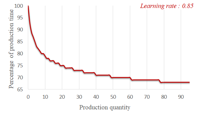
Refer to caption — Figure 1: A straight single-model aircraft assembly line with three workstations. $i+1$ , $i$ , and $i-1$ are successive units being assembled.

Aircraft manufacturing plants are designed to produce at a certain rate. However, once production begins, it takes time for the system to reach this production rate. Workers need to gain experience, improve their skills, improve the supply chain management and optimise the production process. Therefore, the initial production rate of plants is always lower than the target rate, and the difference between the two can be significant. As production progresses, continuous improvements in workflow optimisation, automation integration and experience help to narrow this gap. This phenomenon, known as the learning effect, refers to the gradual improvement in production system efficiency through task repetition, resulting in reduced task durations [38]. The variation in duration based on the repetition of the same task is called a learning curve (Figure 2), and the period in which the task duration continuously improves until it reaches a steady state is referred to as the learning stage. The phase required for the production system to reach the target production rate is called the ramp-up stage, which is currently a challenging topic of great interest in manufacturing [12, 21].

Since the time required to perform a task in a manufacturing environment usually fluctuates over time due to the learning effect, the design of the assembly line and the assembly process is continually refined. However, the stability of an assembly line is also a critical factor, as any change in the production process incurs costs. There are a number of potential causes for this issue, including the time taken to install or deinstall the heavy machines between workstations, errors made by workers when the assembly process changes and becomes unfamiliar, or changes in inventory management and the supply chain, etc. This creates a clear trade-off decision for aircraft manufacturers: pursuit of a continuously optimised assembly line must be weighed against the cost of making changes to the production process. Indeed, if the assembly line is continuously optimised, the production time will consistently decrease, allowing the system to reach the desired production rate more quickly. However, this process also carries an increased risk and higher associated costs due to the greater number of changes being implemented on the line.

In this work, we investigate the use of Constraint Programming (CP) to address the Resource-Constrained Assembly Line Balancing Problem considering the learning effect. We denote this problem as RC-ALBP/L. The decision, made under resource-constrained conditions, involves a trade-off between the ramp-up time – the time required to reach the target production rate or cycle time – and the number of adjustments to the line. This decision includes determining the task and resource allocation to each workstation, as well as setting the cycle time for each production period. Note that while industrial partners have shown strong interest in the challenge of ramping up production on an assembly line, this research has been conducted in an academic setting. Meetings are planned with industrial partners in the near future on this topic.

The paper is structured as follows. After presenting some related works in Section 2, RC-ALBP/L and its encoding in Optimization Programming Language (OPL) [36] are formally introduced in Section 3 and Section 4. The results of the experiments we have performed are presented in Section 5. Finally, we conclude and discuss some perspectives in Section 6.

2 Related Works

The Assembly Line Balancing Problem (ALBP) is a well-known problem in the literature. Starting from the Simple ALBP (SALBP) [20], numerous extensions have been proposed over the years to address its various dimensions [7, 8, 10]. In this study, we specifically focus on Resource-Constrained ALBP (RC-ALBP), scheduling in the presence of the learning effect, and ALBP with the learning effect.

Resource-Constrained ALBP.

This issue has been referred to by a number of names in the past [11, 37], but it was not formally defined until 2005 in [2]. The definition of RC-ALBP was further refined in [16], where the authors pointed out that the resources required by tasks can be simple or multiple, alternative and/or concurrent. The complexity of RC-ALBP has been proven to be strongly NP-hard in [29], even without considering scheduling aspects. When task parallelism is allowed at the workstation level, the decision making process extends beyond task and resource allocation to include the determination of task start times. This particular variant of RC-ALBP has been widely studied under the name Multi-Manned ALBP, which was first introduced in [17]. However, most of these studies still did not consider cumulative resource scheduling, treating each worker as a separate capacity-one resource, and assuming that each task required only one worker. A number of solution approaches have been developed to tackle RC-ALBP, both with and without scheduling considerations, including techniques based on CP [3, 14, 18, 33, 34, 35, 40]. In [14, 35, 40], the authors compared the performance of CP with that of Mixed-Integer Linear Programming (MILP) and some incomplete solution approaches (e.g. Simulated Annealing, Genetic Algorithms). The results showed that CP outperforms the other approaches in this context.

Learning Effect and Scheduling.

The learning effect was first documented in [38], where the author introduced a log-linear learning curve (Figure 2) that we incorporate in our experiments. Since then, numerous types of learning curves have been developed. A historical review and a meta-analysis of various learning curves are available in [19] and [39]. In scheduling environments, learning can be approached in two ways: (a) the position-based approach, where the extent of learning depends on the number of times a task has been carried out; and (b) the sum-of-processing-time approach, which accounts for the total processing time of all similar tasks completed up to that point [9]. There are notable works on the scheduling problem that consider the learning effect. The multi-mode Resource-Constrained Project Scheduling Problem (RCPSP) with learning effect is addressed in [31, 32], where the duration of each task depends on the amount of resources performed on it. In [22], four CP formulations for the RCPSP with the learning effect are introduced, along with an empirical comparison of their scheduling and lower bounding performance. In [26], the authors consider the learning effect in the high-multiplicity RCPSP, where multiple repetitive projects need to be scheduled, using CP and prove the existence of symmetrical solutions in this problem.

ALBP with Learning Effect.

Although ALBP has been widely studied with many extensions, only a few have considered the learning effect and most of them apply the position-based approach. A review of works conducted before 2023 that account for the learning effect in ALBP can be found in [1]. A relaxed version of SALBP with a learning effect (SALBP/L) was first addressed in [15]. The authors proved that the optimal task allocation, while minimising the throughput time of a batch product, is imbalanced in the presence of homogeneous learning. This work has been extended to SALBP/L in [23]. In [30], a modified branch-and-bound algorithm and a fast heuristic based on a task priority rule for SALBP/L, while minimising the number of workstations and the learning stage duration, have been proposed. However, the learning effect is relaxed since the line is considered pre-filled, all tasks have the same number of repetitions in each cycle, and the cycle time can only be changed in predetermined periods. Integer Linear Programming (ILP) and a matheuristic approach, which is based on variable neighborhood search and dynamic programming, have been used to address the same problem in [6]. In [27], the authors provided two rebalancing procedure for SALBP/L to reduce the number of workstations on the line. Nevertheless, this work still considers a relaxed view of the learning effect when counting the number of task repetitions for the position-based learning approach. In fact, a task from a later-entered unit can be processed earlier than one from an earlier unit, and more than one instance of the same task might be processed simultaneously for different units. More recently, mixed-model ALBP incorporating the learning effect has been addressed using ILP and matheuristic approaches, further expanding research in this area [4, 28].

To the best of our knowledge, no work in the literature simultaneously addresses RC-ALBP considering scheduling aspects with task durations dependent on the learning effect. As this is a novel problem, we adopt a complete approach (i.e. an approach able to prove optimality and to provide optimality gaps) in order to establish a baseline. In the literature, it has been shown that CP outperforms MILP in similar problem contexts, which motivates our choice for CP. Our contributions through this work are:

$\blacksquare$

Formally define RC-ALBP/L with an individual learning curve associated with each task.
$\blacksquare$

Propose an OPL encoding for RC-ALBP/L.
$\blacksquare$

Introduce a dominance-breaking method, while proving its correctness.
$\blacksquare$

Identify three solving approaches based on the constraint programming model.
$\blacksquare$

Conduct an experiment on industrial aircraft assembly line benchmarks, allowing us to compare CP-based solving approaches, along with an ILP approach.

3 Problem Description

The assembly line under consideration is single-model and straight. Moreover, due to the nature of the aircraft assembly line, we have included the notion of a zone that represents a subpart of the aircraft in which assembly tasks are performed. Each workstation contains the same set of different zones, either inside or outside the aircraft. Each zone has a capacity and can be treated as a cumulative, renewable resource for task execution. Furthermore, for safety reasons, certain tasks may disable specific zones during their execution. When a zone is disabled, any task that requires it will be unable to proceed. However, tasks that disable the same zone can run simultaneously. In this section, we formally describe the components required to define an instance of the problem we consider, namely RC-ALBP/L, aiming to minimise the ramp-up time and the number of adjustments to the line. We do not consider rebalancing or dynamic task allocation in this work.

3.1 Problem Inputs

An instance of RC-ALBP/L is defined by a tuple consisting of the following elements.

$\blacksquare$

The target cycle time $c_{\mathit{tgt}}$ , which is the cycle time we want to reach.
$\blacksquare$

The maximum value of cycle time $c_{\mathit{max}}$ , which is the longest allowable time between the completion of two consecutive assembled units.
$\blacksquare$

The number of workstations $W$ . We denote $\mathcal{W}=\{1,\dots,W\}$ , or equivalently $\llbracket 1,W\rrbracket$ , as the set of workstations. Workstations are ordered from 1 to $W$ on the line.
$\blacksquare$

The number of periods $P$ . A period is the time interval during which a unit stays at a workstation, and the cycle time in each period corresponds to the duration of this interval. We denote $\mathcal{P}=\llbracket 1,P\rrbracket$ as the set of periods.
$\blacksquare$

The set of tasks $\mathcal{T}$ ( $|\mathcal{T}|=T$ ), with for each task $t\in\mathcal{T}$ , a monotonically decreasing duration function, denoted as $\mathit{dur}_{t}:\mathbb{Z}\to\mathbb{N}$ , which returns the duration of the task based on the number of times it has been completely executed before, or zero if the input is negative. Note that in period number $p$ , the number of complete executions of a task allocated to station number $w$ is $p-w$ . For instance, the duration of a task $t$ allocated to workstation 3 in period 2 is $\mathit{dur}_{t}(2-3)=\mathit{dur}_{t}(-1)=0$ , since workstation 3 is not yet in service during period 2. During period 5, its duration will be $\mathit{dur}_{t}(5-3)=\mathit{dur}_{t}(2)$ , because $t$ has already been executed twice (in periods 3 and 4).
$\blacksquare$

The graph $\mathcal{G}=(\mathcal{T},\mathcal{A})$ represents the precedence relationship between tasks in $\mathcal{T}$ . An arc $(t,u)\in\mathcal{A}$ indicates that task $t$ must be finished before the start of task $u$ .
$\blacksquare$

The set of resources $\mathcal{R}$ , where, for each resource $r\in\mathcal{R}$ , $\mathit{capa}_{r}$ denotes the capacity of $r$ , and $\mathit{cons}_{r,t}$ denotes the amount of resource $r$ consumed by task $t\in\mathcal{T}$ . Resources can typically represent a set of machines or a set of workers that are assigned to a workstation for performing tasks in this workstation.
$\blacksquare$

The set of zones $\mathcal{Z}$ , where, for each zone $z\in\mathcal{Z}$ , $\mathit{capa}_{z}$ denotes the capacity of $z$ , $\mathit{cons}_{z,t}$ denotes the share of zone $z$ occupied by task $t\in\mathcal{T}$ , and $\mathcal{D}_{t}\subseteq\mathcal{Z}$ is the set of zones that are disabled during the execution of task $t$ .
$\blacksquare$

The workstation-relative time horizon, for each task during each period $\mathcal{H}=\llbracket 0,c_{\mathit{max}}\rrbracket$ .

Assumptions.

An instance of RC-ALBP/L is said to be well-formed if and only if the following assumptions hold. Note that unless said otherwise, all instances considered in the paper are supposed to be well-formed.

1.
The number of periods $P$ is greater than the number of workstations $W$ . Under this assumption, the set of periods $\mathcal{P}$ can be partitioned into two subsets:
- $\blacksquare$
  
  $\mathcal{P}^{U}=\llbracket 1,W\rrbracket$ representing the periods when the line is being filled, called unstable periods.
- $\blacksquare$
  
  $\mathcal{P}^{S}=\llbracket W+1,P\rrbracket$ the stable periods.
2.

The cycle time cannot be changed during the unstable fill-up periods (the first $W$ periods). This assumption is made to prevent an increase in cycle time during these periods, particularly when more tasks are assigned to a downstream workstation. Under this assumption, the cycle time during these periods is equal to the maximum cycle time among them.
3.

The cycle time of the unstable periods is greater than the target cycle time.
4.

Any task can be allocated to any workstation. The allocation of a task is the same for all periods (no dynamic task allocation or rebalancing allowed).
5.

A task cannot be split among workstations (non-preemptive tasks).
6.

In each period, all tasks must be completed.
7.

The precedence graph $\mathcal{G}$ is acyclic.
8.

Any resource can be allocated to any workstation. The amount of each resource allocated to each workstation is the same for all periods (no dynamic resource allocation allowed).

Example 1.

We consider a toy example, instance of RC-ALBP/L, consisting of 2 workstations, 2 resources $\{r_{1},r_{2}\}$ , each with a capacity of 6, and a zone $z$ with a capacity of 1. The target cycle time is 12 and the maximum number of periods for the ramp-up is 6. The maximum value for the cycle time is 20. There are 6 tasks, each with an individual learning curve, i.e. durations based on the number of complete executions of the task. The consumption of resources and zone by each task is represented in Figure 3(a). Task $c$ is the only one that disables zone $z$ during its execution. The precedence relationship graph between tasks is represented in Figure 3(b).

Task	Consume			Disable	Duration after $n$ complete executions
	$r_{1}$	$r_{2}$	$z$		$0$	1	2	3	4	5
a	3	1	1	–	9	8	7	6	5	5
b	2	2	1	–	10	7	4	4	4	4
c	1	1	0	$z$	4	4	4	4	4	4
d	0	3	0	–	8	5	3	3	2	2
e	2	1	1	–	7	6	6	5	5	5
f	1	2	0	–	5	5	4	4	3	3

(a) Tasks involved in the toy example.

(b) Precedence relationship.

Figure 3: Tasks features (a) and precedence relationship (b) for the toy example.

3.2 Assignment, Solution and Optimality

Assignment.

An assignment (i.e. a solution attempt) of a RC-ALBP/L instance is defined by a tuple $(\mathit{wks}{},\mathit{raw}{},\mathit{start}{},\mathit{cyc}{})$ , where:

$\blacksquare$

$\mathit{wks}{}:\mathcal{T}\to\mathcal{W}$ is a function that maps, for each task $t\in\mathcal{T}$ , the workstation $w\in\mathcal{W}$ to which it is allocated;
$\blacksquare$

$\mathit{raw}{}:\mathcal{R}{}\times\mathcal{W}\to\mathbb{N}$ is a function that maps, for each pair composed of a resource $r\in\mathcal{R}{}$ and a workstation $w\in\mathcal{W}$ , the amount of resource $r$ allocated to workstation $w$ ;
$\blacksquare$

$\mathit{start}{}:\mathcal{T}\times\mathcal{P}\to\mathbb{N}$ is a function that maps, for each task $t\in\mathcal{T}$ and each period $p\in\mathcal{P}$ , the start time of $t$ in the workstation to which $t$ is allocated during that period $p$ ;
$\blacksquare$

$\mathit{cyc}{}:\mathcal{P}\to\mathbb{N}$ is a function that maps, for each period $p\in\mathcal{P}$ , its cycle time.

We define an additional function $\mathit{end}{}:\mathcal{T}\times\mathcal{P}\to\mathbb{N}$ that maps, for each task and each period, the end time in the workstation to which the task is allocated during that period. For each task $t\in\mathcal{T}$ and each period $p\in\mathcal{P}$ , the value of this function can be calculated as follows:

\displaystyle\mathit{end}{(t,p)}=\mathit{start}{(t,p)}+\mathit{dur}_{t}(p-% \mathit{wks}{(t)})

We also have $\mathcal{E}_{t,p}=\llbracket\mathit{start}{(t,p)},\mathit{end}{(t,p)}\llbracket$ representing the time interval during which the task $t$ is executed in period $p$ .

Solution.

An assignment to a RC-ALBP/L instance is a solution if and only if: it satisfies the precedence constraints (Equations 1 and 2); respects the resources’ capacity (Equations 3 and 4); respects the zones’ capacity (Equation 5); satisfies the zone disabling constraints (Equation 6); and respects the characteristics of the cycle time (Equations 7 and 8).

$\displaystyle\forall(t,u)\in\mathcal{A},$	$\displaystyle\mathit{wks}{(t)}\leq\mathit{wks}{(u)}$	(1)
$\displaystyle\forall(t,u)\in\mathcal{A},\forall p\in\mathcal{P},$	$\displaystyle\bigl{(}\mathit{wks}{(t)}=\mathit{wks}{(u)}\bigr{)}\Rightarrow% \bigl{(}\mathit{end}{(t,p)}\leq\mathit{start}{(u,p)}\bigr{)}$	(2)
$\displaystyle\forall r\in\mathcal{R}{},$	$\displaystyle\sum_{w\in\mathcal{W}}\mathit{raw}{(r,w)}\leq\mathit{capa}_{r}$	(3)
$\displaystyle\forall r\in\mathcal{R}{},\forall w\in\mathcal{W},\forall p\in% \mathcal{P},\forall\tau\in\mathcal{H},$	$\displaystyle\sum_{\begin{subarray}{c}t\in\mathcal{T}:\mathit{wks}{(t)}=w% \wedge\tau\in\mathcal{E}_{t,p}\end{subarray}}\mathit{cons}_{r,t}\leq\mathit{% raw}{(r,w)}$	(4)
$\displaystyle\forall z\in\mathcal{Z},\forall w\in\mathcal{W},\forall p\in% \mathcal{P},\forall\tau\in\mathcal{H},$	$\displaystyle\sum_{\begin{subarray}{c}t\in\mathcal{T}:\mathit{wks}{(t)}=w% \wedge\tau\in\mathcal{E}_{t,p}\end{subarray}}\mathit{cons}_{z,t}\leq\mathit{% capa}_{z}$	(5)
$\displaystyle\forall t\in\mathcal{T},\forall p\in\mathcal{P},\forall\tau\in% \mathcal{H},$	$\displaystyle(\tau\in\mathcal{E}_{t,p})\Rightarrow(\mathcal{O}_{u,\tau}=\emptyset)$	(6)
	$\displaystyle\text{with }\mathcal{O}_{u,\tau}=\{u\in\mathcal{T}\setminus\{t\}% \mid\mathit{wks}{(u)}=\mathit{wks}{(t)},\tau\in\mathcal{E}_{u,p},\exists z\in% \mathcal{D}_{t}:\mathit{cons}_{z,u}>0\}$
$\displaystyle\forall p\in\mathcal{P},$	$\displaystyle\max_{t\in\mathcal{T}}(\mathit{end}{(t,p)})\leq\mathit{cyc}{(p)}$	(7)
$\displaystyle\forall p\in\mathcal{P},$	$\displaystyle c_{\mathit{tgt}}\leq\mathit{cyc}{(p)}\leq c_{\mathit{max}}$	(8)

Optimality.

A solution to a RC-ALBP/L instance is said to be optimal (or Pareto-optimal) if and only if no other solution improves one of the following two optimization criteria without worsening the other: (i) the ramp-up duration (Equation 9), and (ii) the number of adjustments to the line (Equation 10). In this work, we consider that an adjustment to the line is a modification of the cycle time.

	$\displaystyle\sum_{p\in\mathcal{P}:c_{\mathit{tgt}}<\mathit{cyc}{(p)}}\mathit{% cyc}{(p)}$		(9)
	$\displaystyle\sum_{p\in\mathcal{P}^{S}}\bigl{(}\mathit{cyc}{(p-1)}\neq\mathit{% cyc}{(p)}\bigr{)}$		(10)

Example 2.

An optimal solution for the example previously introduced is shown in Figure 4. Tasks $\{a,b\}$ are allocated to workstation 1, while tasks $\{c,d,e,f\}$ are allocated to workstation 2. In workstation 1, the order of tasks remains unchanged throughout the production process. In workstation 2, during period 1, no tasks are performed as the first assembled unit is still in workstation 1. There is no adjustment during period 2 due to Assumption 2 (i.e. no adjustment in unstable periods). The production rate adjustments are made in periods 3 and 5. In period 3, the task schedule (or the task execution order) remains the same as in period 2, but a decision is made to reduce the cycle time, since the station time during this period is reduced due to the learning effect. In period 5, a decision is made to change the order of the tasks and further reduce the cycle time to the target cycle time. The ramp-up time in this example is $(19\times 2)+(15\times 2)=68$ and the number of adjustments to the line is 2.
The complete resource profile for this example is available in the Appendix A (Table 4). Note that in this example the available amount of resource $r_{1}$ is 6, but only a total of 5 is allocated to both workstations. The reason for this is that the unavailability of zone $z$ (either in use or disabled) has prevented the tasks from running in parallel.

Figure 4: Allocation and scheduling of tasks for the toy example.

4 Encoding RC-ALBP/L in OPL

In this section, we transcribe in OPL the general mathematical model given in Subsection 3.2 for RC-ALBP/L, and identify some dominance-breaking constraints.

4.1 A Base Model for RC-ALBP/L

To start, we propose a base model for RC-ALBP/L. The construction of this model involves both interval variables and state functions from OPL. An interval variable represents a period of time during which a task is carried out, including the start and end times, its duration, and its nature (mandatory or optional). An optional task may be omitted in the computed solution to the problem. Note that although there are no optional tasks in RC-ALBP/L, this feature is still used in the modelling step. The start time, end time and duration of an interval variable are respectively accessible through functions $\mathsf{startOf}$ , $\mathsf{endOf}$ and $\mathsf{lengthOf}$ . A state function is a function describing the evolution of a given feature of the environment. In scheduling context, this function can be used to describe the status of a specific resource (in this case, the status of a zone). The possible evolution of this function is constrained by interval variables of the problem using OPL functions (e.g. $\mathsf{alwaysEqual}$ ).

In order to encode in OPL the general mathematical model described in Subsection 3.2, we define the corresponding decision variables for each of the assignment functions as follows:

$\blacksquare$

for each task $t\in\mathcal{T}$ , $\mathit{wks}{(t)}$ is represented by an integer variable $\mathbf{wks}_{t}\in\mathcal{W}$ , which indicates the workstation to which $t$ is allocated.
$\blacksquare$

for each allocated resource $r\in\mathcal{R}{}$ and each workstation $w\in\mathcal{W}$ , $\mathit{raw}{(r,w)}$ is represented by an integer variable $\mathbf{raw}_{r,w}\in\llbracket 0,\mathit{capa}_{r}\rrbracket$ , which indicates the amount of $r$ allocated to $w$ .
$\blacksquare$

for each task $t\in\mathcal{T}$ , each period $p\in\mathcal{P}$ , and each workstation $w\in\mathcal{W}$ , the optional interval variable $\mathbf{itv}_{t,p,w}\in\mathcal{H}$ represents the execution of task $t$ during period $p$ at workstation $w$ . This variable is present only if $t$ is assigned to $w$ , in which case it can express the value returned by $\mathit{start}{(t,p)}$ .
$\blacksquare$

for each period $p\in\mathcal{P}$ , $\mathit{cyc}{(p)}$ is represented by an integer variable $\mathbf{cyc}^{\mathbf{dec}}_{p}\in\llbracket c_{\mathit{tgt}},c_{\mathit{max}}\rrbracket$ , which indicates the decided cycle time value of $p$ .

In addition, we also introduce the following additional variables that are useful for stating some constraints:

$\blacksquare$

for each period $p\in\mathcal{P}$ , the integer variable $\mathbf{cyc}^{\mathbf{req}}_{p}\in\mathcal{H}$ represents the minimum required cycle time value of $p$ (or the maximum end time among tasks during $p$ ). The value of this variable is always less than or equal to $\mathbf{cyc}^{\mathbf{dec}}_{p}$ .
$\blacksquare$

for each period $p\in\mathcal{P}$ , the integer variable $\mathbf{cost}_{p}\in\mathcal{H}$ represents the amount of time contributed by $p$ to the ramp-up duration minimisation objective. This variable has the same value as $\mathbf{cyc}^{\mathbf{dec}}_{p}$ if $\mathbf{cyc}^{\mathbf{dec}}_{p}>c_{\mathit{tgt}}$ , and $0$ otherwise.

There are some other additional variables used to encode the zone constraints (or, more specifically, the state function that evolves the status of each zone over time), but these are not described in this section (because they are not related to our main purpose here, which is to express ramp-up cycle time constraints and to express dominance constraints). A complete description of the model in OPL is provided in the Appendix B. The criteria to be minimised are encoded as follows:

		$\displaystyle\sum_{p\in\mathcal{P}}\mathbf{cost}_{p}$		(11)
		$\displaystyle\sum_{p\in\mathcal{P}^{S}}(\mathbf{cost}_{p-1}\neq\mathbf{cost}_{% p})$		(12)

The first objective (Equation 11) is to minimise the time required for the assembly line to reach the target cycle time (or the ramp-up duration). The second objective (Equation 12) is to minimise the number of adjustments to the cycle time. The addressed problem involves a trade-off: to achieve the target cycle time more rapidly, it is necessary to reduce the cycle time of the line as quickly and as extensively as possible, which results in an increase in the number of adjustments to the cycle time.

In this section, we do not elaborate on how each constraint is encoded using the decision variables mentioned earlier. In fact, most of these constraints are quite standard in scheduling problems or have already been discussed in the literature on assembly lines with CP [26, 33, 34]. However, we provide the constraints associated with the ramp-up cycle time variables, which are novel in this work.

$\displaystyle\qquad\forall p\in\mathcal{P},$	$\displaystyle\mathbf{cyc}^{\mathbf{req}}_{p}=\max_{t\in\mathcal{T},w\in% \mathcal{W}}\mathsf{endOf}(\mathbf{itv}_{t,p,w},0)$	(13)
$\displaystyle\forall p\in\mathcal{P}^{U},$	$\displaystyle\mathbf{cyc}^{\mathbf{dec}}_{p}=\max_{q\in\mathcal{P}^{U}}\mathbf% {cyc}^{\mathbf{req}}_{q}$	(14)
$\displaystyle\forall p\in\mathcal{P}^{S},$	$\displaystyle\mathbf{cyc}^{\mathbf{dec}}_{p}\geq\mathbf{cyc}^{\mathbf{req}}_{p}$	(15)
$\displaystyle\qquad\forall p\in\mathcal{P}^{U},$	$\displaystyle\mathbf{cost}_{p}=\mathbf{cyc}^{\mathbf{dec}}_{p}$	(16)
$\displaystyle\forall p\in\mathcal{P}^{S},$	$\displaystyle(\mathbf{cyc}^{\mathbf{dec}}_{p}>c_{\mathit{tgt}})\Longrightarrow% (\mathbf{cost}_{p}=\mathbf{cyc}^{\mathbf{dec}}_{p})$	(17)
$\displaystyle\forall p\in\mathcal{P}^{S},$	$\displaystyle(\mathbf{cyc}^{\mathbf{dec}}_{p}=c_{\mathit{tgt}})\Longrightarrow% (\mathbf{cost}_{p}=0)$	(18)

The constraints (13) compute the required cycle time for each period. Constraints (14) ensure that the decided cycle time during the unstable periods is equal to the maximum required cycle time among them and cannot be altered during these periods. Constraints (15) express that the decided cycle time during the stable periods is greater than or equal to the required cycle time. Next, the constraints (16), (17) and (18) calculate, for each period, the time contributed to the ramp-up stage. A comprehensive description of this base model with all the constraints is provided in the Appendix B.

4.2 Dominance-Breaking Constraints

We now introduce some dominance-breaking constraints [13] for RC-ALBP/L. With $\mathcal{S}$ representing the solution space of RC-ALBP/L, we can define two functions $\mathit{obj}_{\mathit{ru}}{}:\mathcal{S}\rightarrow\mathbb{N}$ and $\mathit{obj}_{\mathit{na}}{}:\mathcal{S}\rightarrow\mathbb{N}$ that return the value of the objective calculated by Equation 9 and Equation 10, respectively.

Definition 3 (Dominance relation).

For any two solutions $\sigma$ and $\pi$ , a dominance relation $\preceq$ is an incomplete, reflexive and transitive relation between $\sigma$ and $\pi$ , which expresses the following conditions:

\pi\preceq\sigma\Longleftrightarrow(\mathit{obj}_{\mathit{ru}}{(\pi)}\leq% \mathit{obj}_{\mathit{ru}}{(\sigma)})\land(\mathit{obj}_{\mathit{na}}{(\pi)}% \leq\mathit{obj}_{\mathit{na}}{(\sigma)})

The aim of the dominance-breaking constraints is to reduce the solution space from $\mathcal{S}$ to a solution space $\mathcal{S}^{\mathit{dom}}\subseteq\mathcal{S}$ without changing the quality of the optimal solutions. In brief, for every solution $\sigma$ removed by the dominance-breaking constraints, there exists a solution $\pi$ remaining that is at least as good as $\sigma$ in terms of both objectives. Formally:

\forall\sigma\in\mathcal{S}\setminus\mathcal{S}^{\mathit{dom}},\exists\pi\in% \mathcal{S}^{\mathit{dom}}:\pi\preceq\sigma

Next, we provide a detailed description of each dominance-breaking constraint. For convenience, in the remainder of this paper, for any assignment $\sigma$ (see Subsection 3.2) we denote by $\mathit{x}(\sigma)$ the value of a decision variable $\mathit{x}$ corresponding to $\sigma$ (e.g. $\mathbf{cyc}^{\mathbf{dec}}_{p}(\sigma)$ ). Similarly, we denote by $\mathit{f}_{\sigma}$ the value returned by an assignment function $\mathit{f}$ corresponding to $\sigma$ (e.g. $\mathit{start}_{\sigma}{(t,p)}$ ).

Definition 4 ( $p$ -excluded equivalence).

For any two assignments $\sigma$ and $\pi$ , for any period $p\in\mathcal{P}$ , a $p$ -excluded equivalence (noted $\stackrel{{\scriptstyle p}}{{\sim}}$ ) is a symmetrical, reflexive and transitive relation between $\sigma$ and $\pi$ such that all of the following conditions are satisfied:

$\blacksquare$

$\forall t\in\mathcal{T},\;\mathit{wks}_{\pi}{(t)}=\mathit{wks}_{\sigma}{(t)}$ ;
$\blacksquare$

$\forall r\in\mathcal{R}{},\;\forall w\in\mathcal{W},\;\mathit{raw}_{\pi}{(r,w)% }=\mathit{raw}_{\sigma}{(r,w)}$ ;
$\blacksquare$

$\forall t\in\mathcal{T},\;\forall q\in\mathcal{P}\setminus\{p\},\;\mathit{% start}_{\pi}{(t,q)}=\mathit{start}_{\sigma}{(t,q)}$ ;
$\blacksquare$

$\forall q\in\mathcal{P}\setminus\{p\},\;\mathit{cyc}_{\pi}{(q)}=\mathit{cyc}_{% \sigma}{(q)}$ .

Put simply, Definition 4 means that if $\sigma\stackrel{{\scriptstyle p}}{{\sim}}\pi$ , then the only decisions that may differ between $\sigma$ and $\pi$ are the tasks schedule during period $p$ and the cycle time of $p$ . In the following of this section, we focus on creating dominance-breaking rules that enforce $\mathit{cyc}{}$ to become a monotonically decreasing function, which is not necessarily the case for non-optimal solutions.

Lemma 5.

Let $\sigma$ be a solution and $p$ a period in $\mathcal{P}^{S}$ such that $\mathbf{cyc}^{\mathbf{req}}_{p-1}(\sigma{})<\mathbf{cyc}^{\mathbf{req}}_{p}(% \sigma{})$ . There exists a solution $\pi\preceq\sigma$ such that $\mathbf{cyc}^{\mathbf{req}}_{p-1}(\pi)\geq\mathbf{cyc}^{\mathbf{req}}_{p}(\pi)$ .

Proof.

Let $\pi$ an assignment such that $\sigma\stackrel{{\scriptstyle p}}{{\sim}}\pi$ and for any task $t\in\mathcal{T}$ , $\mathit{start}_{\pi}{(t,p-1)}=\mathit{start}_{\pi}{(t,p)}$ . As $\mathit{dur}_{t}(p-1)\geq\mathit{dur}_{t}(p)$ (remember that $\mathit{dur}_{t}$ is a monotonically decreasing function), then $\mathit{end}_{\pi}{(t,p-1)}\geq\mathit{end}_{\pi}{(t,p)}$ and thus $\mathbf{cyc}^{\mathbf{req}}_{p-1}(\pi)\geq\mathbf{cyc}^{\mathbf{req}}_{p}(\pi)$ (see Figure 5). Since $\sigma$ is a solution and $\sigma\stackrel{{\scriptstyle p}}{{\sim}}\pi$ , then all constraints are satisfied in $\pi$ for periods in $\mathcal{P}\setminus\{p\}$ . As i) the start times of tasks during period $p$ in $\pi$ remain the same as during $p-1$ , and ii) the tasks during $p$ are finished earlier than during $p-1$ , then all precedence, resource and zone constraints will be naturally satisfied (they are relaxed).
Since $\mathbf{cyc}^{\mathbf{req}}_{p}(\pi)\leq\mathbf{cyc}^{\mathbf{req}}_{p-1}(\pi)% =\mathbf{cyc}^{\mathbf{req}}_{p-1}(\sigma{})<\mathbf{cyc}^{\mathbf{req}}_{p}(% \sigma{})\leq\mathbf{cyc}^{\mathbf{dec}}_{p}(\sigma)$ , then we can select $\mathbf{cyc}^{\mathbf{dec}}_{p}(\pi)$ such that $\mathbf{cyc}^{\mathbf{dec}}_{p}(\pi)\leq\mathbf{cyc}^{\mathbf{dec}}_{p}(\sigma% )\leq c_{\mathit{max}}$ , which satisfies the cycle time characteristics and makes $\pi$ a solution. As $\sigma\stackrel{{\scriptstyle p}}{{\sim}}\pi$ , we have $\mathbf{cyc}^{\mathbf{dec}}_{q}(\pi)=\mathbf{cyc}^{\mathbf{dec}}_{q}(\sigma)$ for all $q\in\mathcal{P}\setminus\{p\}$ . Two possibilities exist:

$\blacksquare$

if $p$ is not an adjustment period in $\sigma$ , then simply selecting $\mathbf{cyc}^{\mathbf{dec}}_{p}(\pi)=\mathbf{cyc}^{\mathbf{dec}}_{p}(\sigma)$ will make $\pi\preceq\sigma$ .
$\blacksquare$

if $p$ is an adjustment period in $\sigma$ , then any possible value of $\mathbf{cyc}^{\mathbf{dec}}_{p}(\pi)$ such that $\mathbf{cyc}^{\mathbf{dec}}_{p}(\pi)<\mathbf{cyc}^{\mathbf{dec}}_{p}(\sigma)$ will make $\pi\preceq\sigma$ .

We have $\pi\preceq\sigma$ in both cases. Hence, the lemma is proved. $\hfill\blacktriangleleft$

Figure 5: Illustration of Lemma 5’s proof: the task intervals during period

p

in

\pi

are covered by those of period

p-1

.

Lemma 6.

Let $\sigma$ be a solution and $p$ an adjustment period in $\mathcal{P}^{S}$ such that $\mathbf{cyc}^{\mathbf{dec}}_{p-1}(\sigma)<\mathbf{cyc}^{\mathbf{dec}}_{p}(\sigma)$ . There exists a solution $\pi\preceq\sigma$ such that $\mathbf{cyc}^{\mathbf{dec}}_{p-1}(\pi)\geq\mathbf{cyc}^{\mathbf{dec}}_{p}(\pi)$ .

Proof.

There are two possible cases: (a) $\mathbf{cyc}^{\mathbf{req}}_{p-1}(\sigma{})\geq\mathbf{cyc}^{\mathbf{req}}_{p}% (\sigma{})$ ; and (b) $\mathbf{cyc}^{\mathbf{req}}_{p-1}(\sigma{})<\mathbf{cyc}^{\mathbf{req}}_{p}(% \sigma{})$ .
In case (a), since $\mathbf{cyc}^{\mathbf{req}}_{p}(\sigma{})\leq\mathbf{cyc}^{\mathbf{req}}_{p-1}% (\sigma{})\leq\mathbf{cyc}^{\mathbf{dec}}_{p-1}(\sigma)$ , we can construct a solution $\pi$ from $\sigma$ by simply selecting any possible value of $\mathbf{cyc}^{\mathbf{dec}}_{p}(\pi)$ within the interval $\llbracket\mathbf{cyc}^{\mathbf{req}}_{p}(\sigma{}),\mathbf{cyc}^{\mathbf{dec}% }_{p-1}(\sigma)\rrbracket$ , while keeping all other decisions from $\sigma$ unchanged. The solution $\pi$ obtained satisfies $\pi\preceq\sigma$ .
In case (b), based on Lemma 5 proved above, we can construct a solution $\sigma^{\prime}$ such that $\mathbf{cyc}^{\mathbf{req}}_{p-1}(\sigma{{}^{\prime}})\geq\mathbf{cyc}^{% \mathbf{req}}_{p}(\sigma{{}^{\prime}})$ and $\sigma^{\prime}\preceq\sigma$ . From here, the situation reverts back to case (a) mentioned earlier. We follow the procedure in case (a) and construct a solution $\pi$ such that $\pi\preceq\sigma^{\prime}$ , and therefore $\pi\preceq\sigma$ .
In both cases, we can construct a solution $\pi\preceq\sigma$ . Hence, the lemma is proved. $\hfill\blacktriangleleft$

With Lemma 5 and Lemma 6 provided above, we can solely consider solutions where $\mathit{cyc}{}$ is monotonically decreasing. We conclude this section with another dominance-breaking rule, which ensures that the minimum possible cycle time is selected in each adjustment period.

Lemma 7.

Let $\sigma$ be a solution and $p$ an adjustment period in $\mathcal{P}^{S}$ such that $\mathbf{cyc}^{\mathbf{dec}}_{p-1}(\sigma)>\mathbf{cyc}^{\mathbf{dec}}_{p}(\sigma)$ and $\mathbf{cyc}^{\mathbf{dec}}_{p}(\sigma)>\mathbf{cyc}^{\mathbf{req}}_{p}(\sigma% {})$ . There exists a solution $\pi\preceq\sigma$ such that $\mathbf{cyc}^{\mathbf{dec}}_{p}(\pi)=\mathbf{cyc}^{\mathbf{req}}_{p}(\pi)$ .

Proof.

Since $\mathbf{cyc}^{\mathbf{dec}}_{p}(\sigma)>\mathbf{cyc}^{\mathbf{req}}_{p}(\sigma% {})$ , we can construct a solution $\pi$ from $\sigma$ by simply selecting the value of $\mathbf{cyc}^{\mathbf{dec}}_{p}(\pi)=\mathbf{cyc}^{\mathbf{req}}_{p}(\sigma{})$ , while keeping all other decisions from $\sigma$ unchanged. As the ramp-up time in $\pi$ is reduced, we have $\pi\preceq\sigma$ . $\hfill\blacktriangleleft$

From all the proved lemma above, we can safely introduce the following dominance-breaking constraints for RC-ALBP/L:

\halign to=0.0pt{\relax\global\advance\@IEEEeqncolcnt by 1\relax\begingroup% \csname @IEEEeqnarraycolPREr\endcsname#\relax\relax\relax\relax\relax\relax% \relax\relax\relax\relax\csname @IEEEeqnarraycolPOSTr\endcsname\relax\relax% \relax\relax\relax\relax\relax\relax\relax\relax\endgroup&\relax\global% \advance\@IEEEeqncolcnt by 1\relax\begingroup\csname @IEEEeqnarraycolPREc% \endcsname#\relax\relax\relax\relax\relax\relax\relax\relax\relax\relax\csname @IEEEeqnarraycolPOSTc% \endcsname\relax\relax\relax\relax\relax\relax\relax\relax\relax\relax% \endgroup&\relax\global\advance\@IEEEeqncolcnt by 1\relax\begingroup\csname @IEEEeqnarraycolPREc% \endcsname#\relax\relax\relax\relax\relax\relax\relax\relax\relax\relax\csname @IEEEeqnarraycolPOSTc% \endcsname\relax\relax\relax\relax\relax\relax\relax\relax\relax\relax% \endgroup&\global\advance\@IEEEeqncolcnt by 1\relax\bgroup#\egroup&\global% \advance\@IEEEeqncolcnt by 1\relax\hbox to\z@\bgroup\hss#\egroup\cr\hfil$% \displaystyle\forall p \in\mathcal{P}^{S}, $&\hfil$\displaystyle$\hfil&\hfil$% \displaystyle\mathbf{cyc}^{\mathbf{req}}_{p-1} \geq\mathbf{cyc}^{\mathbf{req}}% _{p} $\hfil&{{}\vrule width=0.0pt,height=0.0pt,depth=0.0pt}&0.0pt{\hss(19)}\cr% \penalty 100\vskip 3.0pt\vskip 0.0pt\cr\hfil$\displaystyle\forall p \in% \mathcal{P}^{S}, $&\hfil$\displaystyle$\hfil&\hfil$\displaystyle\mathbf{cyc}^{% \mathbf{dec}}_{p-1} \geq\mathbf{cyc}^{\mathbf{dec}}_{p} $\hfil&{{}\vrule width% =0.0pt,height=0.0pt,depth=0.0pt}&0.0pt{\hss(20)}\cr\penalty 100\vskip 3.0pt% \vskip 0.0pt\cr\hfil$\displaystyle\forall p \in\mathcal{P}^{S}, $&\hfil$% \displaystyle\qquad$\hfil&\hfil$\displaystyle(\mathbf{cyc}^{\mathbf{dec}}_{p-1% } > \mathbf{cyc}^{\mathbf{dec}}_{p}) \Longrightarrow(\mathbf{cyc}^{\mathbf{dec% }}_{p}= \mathbf{cyc}^{\mathbf{req}}_{p}) $\hfil&{\vrule width=0.0pt,height=0.0pt,depth=0.0pt}&0.0pt{\hss(21)}\cr}

The constraints (4.2) and (4.2) ensure that both the required and decided cycle times are never increasing during the stable periods, according to Lemma 5 and 6. Finally, constraints (4.2) guarantee that whenever an adjustment is made, the smallest possible value is selected for the decided cycle time according to Lemma 7.

5 Experimentation

In this section, we present the results of experiments conducted on real-world benchmarks. The details of the benchmarks are provided first, followed by an analysis of the results.

5.1 Benchmarks

Learning Curves.

In this work, we use the log-linear learning curve with a steady learning state [38, 39, 19]. Such a log-linear curve is the classical model used in the aeronautical industry. We define for each task $t\in\mathcal{T}$ : (a) the duration for the first execution $\mathit{dur}_{t}^{0}=\mathit{dur}_{t}(0)$ ; (b) the duration when the learning effect reaches its steady state $\mathit{dur}_{t}^{\infty}$ ; and (c) the learning rate $l_{t}\in\;]0,1]$ which is a parameter that determines the slope of the learning curve. The duration function, based on the number of complete executions $n$ for each task $t$ , is given by the following formula:

\displaystyle\mathit{dur}_{t}(n)=\mathit{dur}_{t}^{\infty}+\bigl{\lceil}(% \mathit{dur}_{t}^{0}-\mathit{dur}_{t}^{\infty})\cdot(n+1)^{\texttt{log}_{2}l_{% t}}\bigr{\rceil},\quad\forall n\in\mathbb{N}

In our experiments, the ratio $\nicefrac{{\mathit{dur}_{t}^{0}}}{{\mathit{dur}_{t}^{\infty}}}$ lies between 2 and 10.

Dataset.

The experiments are conducted on three different datasets that come from real aircraft assembly lines [34]. We have adapted these datasets to account for the learning effect (they are also made available online for further research at [25]). Each dataset consists of 187, 199, and 795 tasks, respectively. The learning rate for each task is randomly selected from the interval $[0.45,1]$ , which is considered a realistic range. Note that using the actual values would not affect the applicability of our approach. For each dataset, we create two instances by varying the number of workstations, the number of periods and the cycle time features as showed in Table 1. A total of six instances were considered. In the remainder of this section, we denote by T-W-P the instance consisting of $T$ tasks, $W$ workstations and $P$ periods (e.g. 199-2-26).

Table 1: Features of data instances: number of tasks, number of workstations, number of periods, target cycle time, maximum value of cycle time, number of resources, capacity of resources, number of zones, capacity of zones, and learning rate.

Solving Approaches.

Due to Assumption 2, the value returned by $\mathit{obj}_{\mathit{na}}{}$ (see Subsection 4.2) for an instance consisting of $W$ workstations and $P$ periods lies in $\llbracket 1,P-W\rrbracket$ . According to Lemma 6, we do not consider an increase in cycle time as part of a possible adjustment to the line, as every solution exhibiting this behaviour is always dominated by a solution with monotonically decreasing cycle time. Therefore, we can transform the original bi-objectives problem into a series of $P-W$ mono-objective sub-problems. For each $m\in\llbracket 1,P-W\rrbracket$ , there is such a sub-problem with constraint (22) and the ramp-up objective (Equation 11).

\displaystyle\sum_{p\in\mathcal{P}^{S}}(\mathbf{cost}_{p-1}>\mathbf{cost}_{p})\leq m

(22)

Such constraints express that the maximum number of adjustments to the cycle time, until the target cycle time is reached, is equal to $m$ . In the experiments, we perform a series of solving attempts (called runs) of the above mono-objective sub-problems using three different solving approaches. Each run is defined by a triplet $(\mathit{I},m,\mathit{A})$ , where $\mathit{I}$ is an instance from the datasets, $m\in\llbracket 1,P-W\rrbracket$ , and $\mathit{A}$ is one of the three following possible solving approaches:

1.

$\mathsf{CPO}$ (baseline solving approach): the base model, as described in Subsection 4.1, is used.
2.

$\mathsf{CPO}^{\mathsf{DB}}$ (dominance-breaking solving approach): the enriched model, which corresponds to the base model together with the dominance-breaking constraints (Equation 4.2, Equation 4.2 and Equation 4.2), is used.
3.

$\mathsf{CPO}^{\mathsf{WS}}$ (warm-start solving approach): the enriched model is used (as for $\mathsf{CPO}^{\mathsf{DB}}$ ), but the solving process involves a kind of incremental mechanism. The aim of $\mathsf{CPO}^{\mathsf{WS}}$ is to directly generate a set of Pareto-optimal solutions. Actually, it can be easily proved that any solution to an instance $\mathit{I}$ with the upper-bound value $m-1$ is also a solution for $\mathit{I}$ with the upper-bound value $m$ . Formally, for all $m>1$ , the final solution returned by ( $\mathit{I},m-1,$ $\mathsf{CPO}^{\mathsf{WS}}$ ) is used to warm-start ( $\mathit{I},m,$ $\mathsf{CPO}^{\mathsf{WS}}$ ), which means that $\mathsf{CPO}^{\mathsf{WS}}$ can only improve the value of the ramp-up objective $\mathit{obj}_{\mathit{ru}}{}$ when $m$ increases.

The numbers of variables and constraints considered in the base model are given in Table 2. As the number of tasks increases, the numbers of variables and constraints both grow at an approximately proportional rate. The same phenomenon occurs when we increase the number of workstations and periods (doubling them results in nearly quadrupling the number of variables and constraints).

Table 2: Number of variables and constraints in the base model (

\mathsf{CPO}

) for each instance.

Instances	187-2-26	199-2-26	795-2-26	187-4-50	199-4-50	795-4-50
# Variables	$12,497$	$13,133$	$44,721$	$47,361$	$49,773$	$169,569$
# Constraints	$61,176$	$75,524$	$235,839$	$234,328$	$288,932$	$901,831$

For comparison purposes, we also evaluated an ILP approach. The chosen ILP formulation is a discrete-time, time-indexed variable encoding. Other MILP encodings exist in the context of resource-constrained scheduling, using sequencing or event-based variables [5]. However, in presence of learning effect, task durations become variables, making those encodings non-linear (they require multiplying decision variables by task durations). Our ILP approach is not described in the main paper because of its poor performance. In fact, due to the explosion in the number of variables and constraints (e.g., 560 million variables and 80 million constraints for the smallest instance, 187-2-26; see Table 5 in the Appendix for other instances), the ILP approach cannot build a relaxed version of the model after running for 2 hours, and even causes the test computer to run out of memory. Details of this approach are provided in the Appendix C.

Test Setup.

The tests have been launched using IBM CP Optimizer 22.1.2 for the CP-based approaches and IBM CPLEX 22.1.2 for the ILP approach [24] through the DOcplex API, on Intel^® Xeon^® CPU E5-2660v3 2.60-3.30 GHz with 62 GB of RAM. We tried several search strategies for all CP-based approaches (e.g., priority branching on cycle time variables, selecting values of variable domains in increasing order, etc.), however, the results obtained were worse than those of the default strategy. Therefore, we chose to retain the default setting. As the number of variables and constraints increases significantly with the number of workstations and periods, the timeout for each run of a 2-workstation instance was set to $900$ seconds (15 minutes), and for a 4-workstation instance, it was set to $7,200$ seconds (2 hours).

5.2 Results

[Uncaptioned image] — Table 3: Comparison between the results of all solving approaches (circle $\bullet$ for $\mathsf{CPO}$ , triangle $\blacktriangledown$ for $\mathsf{CPO}^{\mathsf{DB}}$ , and star $\bigstar$ for $\mathsf{CPO}^{\mathsf{WS}}$ ). Each bigger coloured point represents a non-dominated solution, whereas each small black point corresponds to a dominated one. The vertical axis represents the ramp-up duration, and the horizontal axis represents the actual number of cycle time adjustments.

The results are presented in Table 3. More precisely, for each instance $\mathit{I}$ , we provide a figure representing the results of runs $(\mathit{I},m,\mathit{A})$ , for all $m\in\llbracket 1,P-W\rrbracket$ and for all approaches $A$ . In such figures, each point (circle $\bullet$ for $\mathsf{CPO}$ , triangle $\blacktriangledown$ for $\mathsf{CPO}^{\mathsf{DB}}$ , and star $\bigstar$ for $\mathsf{CPO}^{\mathsf{WS}}$ ) corresponds to a solution for which the vertical axis represents the ramp-up duration (objective $\mathit{obj}_{\mathit{ru}}{}$ ) and the horizontal axis represents the actual number of cycle time adjustments (objective $\mathit{obj}_{\mathit{na}}{}$ ). Note that it is possible to have multiple ramp-up duration values for a given number of adjustments. This means that several values of $m$ (upper bound for objective $\mathit{obj}_{\mathit{na}}{}$ ) have permitted to reach the same value of $\mathit{obj}_{\mathit{na}}{}$ . Non-dominated and dominated solutions (defined relative to each solving approach) are respectively represented with big-coloured and small-black points. Note that solutions which are non-dominated within a given approach may become dominated in a competitive cross-approach comparison.

We begin our analysis by comparing $\mathsf{CPO}$ and $\mathsf{CPO}^{\mathsf{DB}}$ , and we discuss next the results obtained with $\mathsf{CPO}^{\mathsf{WS}}$ .

5.2.1 Comparison Between CPO and CPO^DB

The results corresponding to the solving approaches $\mathsf{CPO}$ and $\mathsf{CPO}^{\mathsf{DB}}$ are represented by circle $\bullet$ and triangle $\blacktriangledown$ in Table 3. There is no clear difference between $\mathsf{CPO}$ and $\mathsf{CPO}^{\mathsf{DB}}$ in terms of solution quality. Both yield a GAP²²2The difference between the objective value of a given solution $\sigma$ and a lower bound LB computed by the solver, typically expressed as a percentage. GAP $(\sigma)$ = $\nicefrac{{(\mathit{obj}_{\mathit{ru}}{}(\sigma)-\mathit{LB})}}{{\mathit{obj}_% {\mathit{ru}}{}(\sigma)}}$ value that exceed 60% in the majority of runs. The figures (embedded in the cells of the table) show that, with these two solving approaches, a greater upper bound for the number of cycle time adjustments (objective $\mathit{obj}_{\mathit{na}}{}$ ) does not guarantee to get a better ramp-up value (objective $\mathit{obj}_{\mathit{ru}}{}$ ) within the given timeouts, except for instance 187-4-50.

Note that optimality was proved for both solving approaches on some runs concerning the instance 187-4-50, using a very small effective tolerance ( $\mathsf{CPO}$ yielding a slightly greater number of proved optimal solutions, yet). In most cases, $\mathsf{CPO}$ and $\mathsf{CPO}^{\mathsf{DB}}$ yields a similar number of competitive non-dominated solutions. However, an exception is observed for the 795-tasks dataset, particularly for the instance 795-2-26, where $\mathsf{CPO}$ significantly outperforms $\mathsf{CPO}^{\mathsf{DB}}$ . Unfortunately, it is worthwhile to note that some solutions produced by $\mathsf{CPO}$ within the allotted time violate Lemma 6, i.e. there are some periods $p$ for which $\mathbf{cyc}^{\mathbf{dec}}_{p-1}<\mathbf{cyc}^{\mathbf{dec}}_{p}$ . As such solutions would not be acceptable in an industrial setting, it means that $\mathsf{CPO}$ would require a post-processing phase in order to satisfy Lemma 6, whereas $\mathsf{CPO}^{\mathsf{DB}}$ provides directly acceptable solutions, even with short timeout values.

5.2.2 Results Obtained with CPO^WS

We recall that the aim of the solving approach $\mathsf{CPO}^{\mathsf{WS}}$ is to directly generate a Pareto-front, as neither $\mathsf{CPO}$ nor $\mathsf{CPO}^{\mathsf{DB}}$ are suited to do so within the specified timeouts except for instances 187-4-50 and 795-2-26.

The results show that $\mathsf{CPO}^{\mathsf{WS}}$ (represented by star $\bigstar$ in Table 3) is actually capable of generating such a Pareto-front for most instances. Moreover, the Pareto-front obtained with $\mathsf{CPO}^{\mathsf{WS}}$ contains more points than the other solving approaches, which allows a finer analysis of the results. For example, for instance 187-4-50, $\mathsf{CPO}^{\mathsf{WS}}$ allows us to evaluate the gain of each additional cycle time adjustment for $m\in\llbracket 1,6\rrbracket$ , whereas solutions computed with $\mathsf{CPO}$ for $m=4$ or $m=6$ are dominated. The optimal ramp-up time is also proved only for this instance, under a very small effective tolerance. $\mathsf{CPO}^{\mathsf{WS}}$ also yields a lower average GAP value compared to the other solving approaches.

That said, $\mathsf{CPO}^{\mathsf{WS}}$ has some drawbacks. First, warm-starting from the solution of the previous run might guide the solver into a part of the search space with lower quality solutions. This is for example the case for instance 795-2-26 where better solutions are found by $\mathsf{CPO}$ and $\mathsf{CPO}^{\mathsf{DB}}$ for low values of $m$ . Another drawback of $\mathsf{CPO}^{\mathsf{WS}}$ lies in the requirement for a sequential execution of all runs, which may lead to very significant extended computational time, whereas each run in $\mathsf{CPO}$ and $\mathsf{CPO}^{\mathsf{DB}}$ can be executed in parallel. However, we also observe that most of the descent in the search tree is concentrated in the first few runs, where solutions improve frequently. This suggests that computational time could probably be reduced by executing the first few runs with the full time allowance, and decreasing the timeout for subsequent runs. However, setting a value to these different time-outs might be strongly linked to the instances and we have not explored that option in this work.

6 Conclusion

In this work, we have a) formally defined the RC-ALBP/L, b) introduced an OPL encoding while providing some dominance-breaking rules for this problem, and c) conducted an experimentation on industrial aircraft assembly line benchmarks using three different CP-based solving approaches.

Since RC-ALBP/L involves a trade-off between ramp-up time and the number of line adjustments, the aim of this work is to generate a Pareto-front, which can be achieved using our solution approaches within a reasonable time limit. These results can provide valuable insights for manufacturers in the design and planning of assembly lines – not only in the aircraft industry, but in production more broadly – especially as minimising ramp-up time is receiving growing attention from them.

In future research, we could explore other solving methods, such as MaxSAT or metaheuristics. We could also investigate scenarios in which the learning effect is transferable across similar tasks, for example installing the left and right wings of an aircraft. Exploring the impact of uncertainty in learning efficiency would allow us to handle robustness issues. Finally, it would be possible to consider that resources are not all available at the beginning of the ramp-up, but are gradually added, therefore adding another level of decision.

References

[1] Z.Z. El Abidine and T. Koltai. The effect of learning on assembly line balancing: A review. Periodica Polytechnica Social and Management Sciences, 2023.
[2] K. Ağpak and H. Gökçen. Assembly line balancing: Two resource constrained cases. International Journal of Production Economics, 96(1):129–140, 2005.
[3] H.M. Alakaş, M. Pınarbaşı, and M. Yüzükırmızı. Constraint programming model for resource-constrained assembly line balancing problem. Soft Computing, 24:5367–5375, 2020. doi:10.1007/S00500-019-04294-8.
[4] E. Alhomaidhi. Enhancing efficiency and adaptability in mixed model line balancing through the fusion of learning effects and worker prerequisites. International Journal of Industrial Engineering Computations, 15(2):541–552, 2024.
[5] C. Artigues, S. Hartmann, and M. Vanhoucke. Fifty years of research on resource-constrained project scheduling explored from different perspectives. European Journal of Operational Research, 2025.
[6] Z. Bao and L. Chen. A matheuristic approach for the aircraft final assembly line balancing problem considering learning curve. In 2023 IEEE International Conference on Industrial Engineering and Engineering Management (IEEM), pages 1389–1393. IEEE, 2023. doi:10.1109/IEEM58616.2023.10407009.
[7] O. Battaïa and A. Dolgui. A taxonomy of line balancing problems and their solution approaches. International Journal of Production Economics, 142(2):259–277, 2013.
[8] O. Battaïa and A. Dolgui. Hybridizations in line balancing problems: A comprehensive review on new trends and formulations. International Journal of Production Economics, 250:108673, 2022.
[9] D. Biskup. A state-of-the-art review on scheduling with learning effects. European Journal of Operational Research, 188(2):315–329, 2008. doi:10.1016/J.EJOR.2007.05.040.
[10] N. Boysen, P. Schulze, and A. Scholl. Assembly line balancing: What happened in the last fifteen years? European Journal of Operational Research, 301(3):797–814, 2022. doi:10.1016/J.EJOR.2021.11.043.
[11] J. Bukchin and M. Masin. Multi-objective design of team oriented assembly systems. European Journal of Operational Research, 156(2):326–352, 2004. doi:10.1016/S0377-2217(03)00054-7.
[12] R. Bultó, E. Viles, and R. Mateo. Overview of ramp-up curves: A literature review and new challenges. Proceedings of the Institution of Mechanical Engineers, Part B: Journal of Engineering Manufacture, 232(5):755–765, 2018.
[13] G. Chu and P. Stuckey. Dominance breaking constraints. Constraints, 20:155–182, 2015. doi:10.1007/S10601-014-9173-7.
[14] Z.A. Çil and D. Kizilay. Constraint programming model for multi-manned assembly line balancing problem. Computers & Operations Research, 124:105069, 2020. doi:10.1016/J.COR.2020.105069.
[15] Y. Cohen, G. Vitner, and S.C. Sarin. Optimal allocation of work in assembly lines for lots with homogenous learning. European Journal of Operational Research, 168(3):922–931, 2006. Balancing Assembly and Transfer lines. doi:10.1016/J.EJOR.2004.07.037.
[16] A. Corominas, L. Ferrer, and R. Pastor. Assembly line balancing: general resource-constrained case. International Journal of Production Research, 49(12):3527–3542, 2011.
[17] S.G. Dimitriadis. Assembly line balancing and group working: A heuristic procedure for workers’ groups operating on the same product and workstation. Computers & Operations Research, 33(9):2757–2774, 2006. Part Special Issue: Anniversary Focused Issue of Computers & Operations Research on Tabu Search. doi:10.1016/J.COR.2005.02.027.
[18] E.B. Edis. Constraint programming approaches to disassembly line balancing problem with sequencing decisions. Computers & Operations Research, 126:105111, 2021. doi:10.1016/J.COR.2020.105111.
[19] E.H. Grosse, C.H. Glock, and S. Müller. Production economics and the learning curve: A meta-analysis. International Journal of Production Economics, 170:401–412, 2015.
[20] W.B. Helgeson and D.P. Birnie. Assembly line balancing using the ranked positional weight technique. Journal of industrial engineering, 12(6):394–398, 1961.
[21] J. Heraud, K. Medini, and A.L. Andersen. Managing agile ramp-up projects in manufacturing–status quo and recommendations. CIRP Journal of Manufacturing Science and Technology, 45:125–137, 2023.
[22] A. Hill, J. Ticktin, and T.W.M. Vossen. A computational study of constraint programming approaches for resource-constrained project scheduling with autonomous learning effects. In Integration of Constraint Programming, Artificial Intelligence, and Operations Research: 18th International Conference, CPAIOR 2021, Vienna, Austria, July 5–8, 2021, Proceedings 18, pages 26–44. Springer, 2021. doi:10.1007/978-3-030-78230-6_2.
[23] T. Koltai and N. Kalló. Analysis of the effect of learning on the throughput-time in simple assembly lines. Computers & Industrial Engineering, 111:507–515, 2017. doi:10.1016/J.CIE.2017.03.034.
[24] P. Laborie, J. Rogerie, P. Shaw, and P. Vilím. IBM ILOG CP optimizer for scheduling: 20+ years of scheduling with constraints at IBM/ILOG. Constraints, 23:210–250, 2018. doi:10.1007/S10601-018-9281-X.
[25] D.A. Le, S. Roussel, and C. Lecoutre. Dataset for the assembly line balancing problem with learning effect, 2025. doi:10.57745/EBDN5W.
[26] D.A. Le, S. Roussel, C. Lecoutre, and A. Chan. Learning Effect and Compound Activities in High Multiplicity RCPSP: Application to Satellite Production. In 30th International Conference CP, 2024. doi:10.4230/LIPIcs.CP.2024.18.
[27] Y. Li and T.O. Boucher. Assembly line balancing problem with task learning and dynamic task reassignment. The International Journal of Advanced Manufacturing Technology, 88:3089–3097, 2017.
[28] Y. Li, D. Liu, and I. Kucukkoc. Mixed-model assembly line balancing problem considering learning effect and uncertain demand. Journal of Computational and Applied Mathematics, 422:114823, 2023. doi:10.1016/J.CAM.2022.114823.
[29] D. Ogan and M. Azizoglu. A branch and bound method for the line balancing problem in u-shaped assembly lines with equipment requirements. Journal of Manufacturing Systems, 36:46–54, 2015.
[30] C. Otto and A. Otto. Extending assembly line balancing problem by incorporating learning effects. International Journal of Production Research, 52(24):7193–7208, 2014.
[31] V. Van Peteghem and M. Vanhoucke. A genetic algorithm for the preemptive and non-preemptive multi-mode resource-constrained project scheduling problem. European Journal of Operational Research, 201(2):409–418, 2010. doi:10.1016/J.EJOR.2009.03.034.
[32] V. Van Peteghem and M. Vanhoucke. Influence of learning in resource-constrained project scheduling. Computers & Industrial Engineering, 87:569–579, 2015. doi:10.1016/J.CIE.2015.06.007.
[33] X. Pucel and S. Roussel. Constraint Programming Model for Assembly Line Balancing and Scheduling with Walking Workers and Parallel Stations. In Paul Shaw, editor, 30th International Conference on Principles and Practice of Constraint Programming (CP 2024), volume 307, pages 23:1–23:21, 2024. doi:10.4230/LIPICS.CP.2024.23.
[34] S. Roussel, T. Polacsek, and A. Chan. Assembly line preliminary design optimization for an aircraft. In CP 2023 (The 29th International Conference on Principles and Practice of Constraint Programming), 2023. doi:10.4230/LIPIcs.CP.2023.32.
[35] K.E. Stecke and M. Mokhtarzadeh. Balancing collaborative human–robot assembly lines to optimise cycle time and ergonomic risk. International Journal of Production Research, 60(1):25–47, 2022. doi:10.1080/00207543.2021.1989077.
[36] P. van Hentenryck. The OPL Optimization Programming Language. The MIT Press, 1999.
[37] J.M. Wilson. Formulation of a problem involving assembly lines with multiple manning of work stations. International Journal of Production Research, 24(1):59–63, 1986.
[38] T.P. Wright. Factors affecting the cost of airplanes. Journal of the aeronautical sciences, 3(4):122–128, 1936.
[39] L.E. Yelle. The learning curve: Historical review and comprehensive survey. Decision sciences, 10(2):302–328, 1979.
[40] Z.A. ÇİL. An exact solution method for multi-manned disassembly line design with and/or precedence relations. Applied Mathematical Modelling, 99:785–803, 2021. doi:10.1016/j.apm.2021.07.013.

Appendix A Resource Profile of Example 2

Table 4: Resource profiles of workstations 1 and 2 (WS1 and WS2) of Example 2.

Period	Resource profile WS1	Resource profile WS2
1
2
3
4
5
6

Appendix B A Base Model in OPL for RC-ALBP/L (Full Version)

The decision variables are the following:

$\blacksquare$

For each task $t\in\mathcal{T}$ , the integer variable $\mathbf{wks}_{t}\in\llbracket 1,W\rrbracket$ indicates the workstation to which $t$ is allocated.
$\blacksquare$

For each allocated resource $r\in\mathcal{R}{}$ and each workstation $w\in\mathcal{W}$ , the integer variable $\mathbf{raw}_{r,w}\in\llbracket 0,\mathit{capa}_{r}\rrbracket$ indicates the amount of $r$ allocated to $w$ .
$\blacksquare$

For each task $t\in\mathcal{T}$ , each period $p\in\mathcal{P}$ and each workstation $w\in\mathcal{W}$ , the optional interval variable $\mathbf{itv}_{t,p,w}\in\mathcal{H}$ represents the execution of task $t$ during the period $p$ at the workstation $w$ . This variable is present only if $t$ is assigned to $w$ .
$\blacksquare$

For each period $p\in\mathcal{P}$ , the integer variable $\mathbf{cyc}^{\mathbf{req}}_{p}\in\mathcal{H}$ indicates the minimum required cycle time value of $p$ (or the maximum end times among tasks time during $p$ ).
$\blacksquare$

For each period $p\in\mathcal{P}$ , the integer variable $\mathbf{cyc}^{\mathbf{dec}}_{p}\in\llbracket c_{\mathit{tgt}},c_{\mathit{max}}\rrbracket$ indicates the decided cycle time value of $p$ (or the cycle time applied to the line during $p$ , which is no less than the required cycle time $\mathbf{cyc}^{\mathbf{req}}_{p}$ ). Note that the value of this variable is also the value returned by the assignment function $\mathit{cyc}{(p)}$ (see Subsection 3.2).
$\blacksquare$

For each period $p\in\mathcal{P}$ , the integer variable $\mathbf{cost}_{p}\in\mathcal{H}$ indicates the amount of time contributed by $p$ to the ramp-up duration minimisation objective. This variable has the same value as $\mathbf{cyc}^{\mathbf{dec}}_{p}$ if $\mathbf{cyc}^{\mathbf{dec}}_{p}>c_{\mathit{tgt}}$ , and $0$ otherwise.
$\blacksquare$

For each zone $z\in\mathcal{Z}$ , each period $p\in\mathcal{P}$ and each workstation $w\in\mathcal{W}$ , the state function $\mathbf{zst}_{z,p,w}$ represents the status of zone $z$ during the periods $p$ at the workstation $w$ .

Constraints and criteria are encoded as follows:

$\mathit{minimise}$

		$\displaystyle\sum_{p\in\mathcal{P}}\mathbf{cost}_{p}$		(23)
		$\displaystyle\sum_{p\in\mathcal{P}^{S}}(\mathbf{cost}_{p-1}\neq\mathbf{cost}_{% p})$		(24)

$\mathit{such\>that}$

$\displaystyle\forall t\in\mathcal{T},\forall p\in\mathcal{P},\forall w\in% \mathcal{W},$	$\displaystyle\mathsf{presenceOf}(\mathbf{itv}_{t,p,w})=\mathsf{equal}(\mathbf{% wks}_{t},w)$	(25)
$\displaystyle\forall p\in\mathcal{P},$	$\displaystyle\mathbf{cyc}^{\mathbf{req}}_{p}=\max_{t\in\mathcal{T},w\in% \mathcal{W}}\mathsf{endOf}(\mathbf{itv}_{t,p,w},0)$	(26)
$\displaystyle\forall p\in\mathcal{P}^{U},$	$\displaystyle\mathbf{cyc}^{\mathbf{dec}}_{p}=\max_{q\in\mathcal{P}^{U}}\mathbf% {cyc}^{\mathbf{req}}_{q}$	(27)
$\displaystyle\forall p\in\mathcal{P}^{S},$	$\displaystyle\mathbf{cyc}^{\mathbf{dec}}_{p}\geq\mathbf{cyc}^{\mathbf{req}}_{p}$	(28)
$\displaystyle\forall p\in\mathcal{P}^{U},$	$\displaystyle\mathbf{cost}_{p}=\mathbf{cyc}^{\mathbf{dec}}_{p}$	(29)
$\displaystyle\forall p\in\mathcal{P}^{S},$	$\displaystyle(\mathbf{cyc}^{\mathbf{dec}}_{p}>c_{\mathit{tgt}})\Longrightarrow% (\mathbf{cost}_{p}=\mathbf{cyc}^{\mathbf{dec}}_{p})$	(30)
$\displaystyle\forall p\in\mathcal{P}^{S},$	$\displaystyle(\mathbf{cyc}^{\mathbf{dec}}_{p}=c_{\mathit{tgt}})\Longrightarrow% (\mathbf{cost}_{p}=0)$	(31)
$\displaystyle\forall(t,u)\in\mathcal{A},$	$\displaystyle\mathbf{wks}_{t}\leq\mathbf{wks}_{u}$	(32)
$\displaystyle\forall(t,u)\in\mathcal{A},\forall p\in\mathcal{P},\forall w\in% \mathcal{W},$	$\displaystyle\mathsf{endBeforeStart}(\mathbf{itv}_{t,p,w},\mathbf{itv}_{u,p,w})$	(33)
$\displaystyle\forall t\in\mathcal{T},\forall p\in\mathcal{P},\forall w\in% \mathcal{W},$	$\displaystyle\mathsf{lengthOf}(\mathbf{itv}_{t,p,w},\mathit{dur}_{t}(p-w))=% \mathit{dur}_{t}(p-w)$	(34)
$\displaystyle\forall r\in\mathcal{R}{},$	$\displaystyle\sum_{w\in\mathcal{W}}\mathbf{raw}_{r,w}\leq\mathit{capa}_{r}$	(35)
$\displaystyle\forall r\in\mathcal{R}{},\forall p\in\mathcal{P},\forall w\in% \mathcal{W},$	$\displaystyle\sum_{t\in\mathcal{T}}\mathsf{pulse}(\mathbf{itv}_{t,p,w},\mathit% {cons}_{r,t})\leq\mathbf{raw}_{r,w}$	(36)

$\displaystyle\forall z\in\mathcal{Z},\forall p\in\mathcal{P},\forall w\in% \mathcal{W},$	$\displaystyle\sum_{t\in\mathcal{T}}\mathsf{pulse}(\mathbf{itv}_{t,p,w},\mathit% {cons}_{z,t})\leq\mathit{capa}_{z}$	(37)
$\displaystyle\forall z\in\mathcal{Z},\forall p\in\mathcal{P},\forall w\in% \mathcal{W},\forall t\in\mathcal{T}:z\in\mathcal{D}_{t},$	$\displaystyle\mathsf{alwaysEqual}(\mathbf{zst}_{z,p,w},\mathbf{itv}_{t,p,w},0)$	(38)
$\displaystyle\forall z\in\mathcal{Z},\forall p\in\mathcal{P},\forall w\in% \mathcal{W},\forall t\in\mathcal{T}:\mathit{cons}_{z,t}>0,$	$\displaystyle\mathsf{alwaysEqual}(\mathbf{zst}_{z,p,w},\mathbf{itv}_{t,p,w},1)$	(39)

The first objective (Equation 23) is to minimize the time required for the assembly line to reach the target cycle time (or the ramp-up duration). The second objective (Equation 24) is to minimize the number of adjustments to the cycle time. The addressed problem involves a trade-off: if we want to reach the target cycle time faster, we need to reduce the cycle time of the line as soon as possible and as much as possible. The constraints (25) link the presence of interval variables with the allocation of tasks. Constraints (26) compute the required cycle time for each period. Constraints (27) ensure that the decided cycle time during the unstable periods remains fixed and is equal to the maximum required cycle time among them. Constraints (28) stipulate that the decided cycle time during the stable periods is greater or equal to the required cycle time. Next, the constraints (29), (30) and (31) calculate, for each period, the time contributed to the ramp-up stage. The precedence relations are handled by the constraints (32) and (33). Constraints (34) calculate the duration for each task in each period. Constraints (35) ensure that the total amount of each resource assigned to all workstations does not exceed its capacity, and constraints (36) enforce cumulative resource limitations at the workstation level. Constraints (37) are cumulative constraints on zone capacity. Finally, the status of the zones during task executions are ensured by constraints (38) and (39).

Appendix C A ILP Model for RC-ALBP/L

C.1 ILP Formulation

As explained in the main paper, in this work, we use a discrete-time, time-indexed variable ILP encoding for RC-ALBP/L. Other MILP encodings exist in the context of resource-constrained scheduling, using sequencing or event-based variables [5]. However, in presence of learning effect, task durations become variables, making those encodings non-linear (they require multiplying decision variables by task durations).

We first provide a MILP encoding for a relaxed version of the problem. For each task $t\in\mathcal{T}$ , each period $p\in\mathcal{P}$ , each workstation $w\in\mathcal{W}$ and each time index $i\in\mathcal{H}$ , we define the following decision variables:

	$\displaystyle\mathbf{wks}_{t,w}$	$\displaystyle=\begin{cases}1&\text{if task $t$ is allocated to workstation $w$% }\\ 0&\text{otherwise}\end{cases}$
	$\displaystyle\mathbf{start}_{t,p,w,i}$	$\displaystyle=\begin{cases}1&\text{if task $t$ starts at time $i$ during % period $p$ in workstation $w$}\\ 0&\text{otherwise}\end{cases}$
	$\displaystyle\mathbf{end}_{t,p,w,i}$	$\displaystyle=\begin{cases}1&\text{if task $t$ ends at time $i$ during period % $p$ in workstation $w$}\\ 0&\text{otherwise}\end{cases}$
	$\displaystyle\mathbf{raw}_{r,w}$	$\displaystyle\in\llbracket 0,\mathit{capa}_{r}\rrbracket\text{ the amount of % resource $r$ allocated to workstation $w$}$
	$\displaystyle\mathbf{cyc}^{\mathbf{req}}_{p}$	$\displaystyle\in\mathcal{H}\text{ the minimum required cycle time value of % period $p$}$
	$\displaystyle\mathbf{cyc}^{\mathbf{dec}}_{p}$	$\displaystyle\in\llbracket c_{\mathit{tgt}},c_{\mathit{max}}\rrbracket\text{ % the decided cycle time value of period $p$}$

	$\displaystyle\mathbf{cost}_{p}$	$\displaystyle\in\mathcal{H}\text{ the amount of time contributed by period $p$% to the ramp-up duration}$
	$\displaystyle\mathbf{target}_{p}$	$\displaystyle=\begin{cases}1&\text{if the target cycle time is not achieved (% or $\mathbf{cyc}^{\mathbf{dec}}_{p}>c_{\mathit{tgt}}$)}\\ 0&\text{otherwise}\end{cases}$

Constraints are encoded as follows:

$\displaystyle\forall t\in\mathcal{T},\forall p\in\mathcal{P},$	$\displaystyle\sum_{w\in\mathcal{W}}\sum_{i\in\mathcal{H}}\mathbf{start}_{t,p,w% ,i}=1$	(40)
$\displaystyle\forall t\in\mathcal{T},\forall p\in\mathcal{P},$	$\displaystyle\sum_{w\in\mathcal{W}}\sum_{i\in\mathcal{H}}\mathbf{end}_{t,p,w,i% }=1$	(41)
$\displaystyle\forall t\in\mathcal{T},$	$\displaystyle\sum_{w\in\mathcal{W}}\mathbf{wks}_{t,w}=1$	(42)
$\displaystyle\forall t\in\mathcal{T},\forall p\in\mathcal{P},\forall w\in% \mathcal{W},$	$\displaystyle\sum_{i\in\mathcal{H}}\mathbf{start}_{t,p,w,i}=\mathbf{wks}_{t,w}$	(43)
$\displaystyle\forall t\in\mathcal{T},\forall p\in\mathcal{P},\forall w\in% \mathcal{W},$	$\displaystyle\sum_{i\in\mathcal{H}}\mathbf{end}_{t,p,w,i}=\mathbf{wks}_{t,w}$	(44)
$\displaystyle\forall t\in\mathcal{T},\forall p\in\mathcal{P},\forall w\in% \mathcal{W},$	$\displaystyle\sum_{i\in\mathcal{H}}i\times\mathbf{end}_{t,p,w,i}\leq\mathbf{% cyc}^{\mathbf{req}}_{p}$	(45)
$\displaystyle\forall p\in\mathcal{P},$	$\displaystyle\mathbf{cyc}^{\mathbf{dec}}_{p}\geq\mathbf{cyc}^{\mathbf{req}}_{p}$	(46)
$\displaystyle\forall p\in\mathcal{P}^{U}\setminus\{1\},$	$\displaystyle\mathbf{cyc}^{\mathbf{dec}}_{p-1}=\mathbf{cyc}^{\mathbf{dec}}_{p}$	(47)
$\displaystyle\forall p\in\mathcal{P}^{S},$	$\displaystyle\mathbf{cyc}^{\mathbf{dec}}_{p}\geq(1+c_{\mathit{tgt}})\times% \mathbf{target}_{p}$	(48)
$\displaystyle\forall p\in\mathcal{P}^{S},$	$\displaystyle\mathbf{cyc}^{\mathbf{dec}}_{p}\leq c_{\mathit{tgt}}+c_{\mathit{% max}}\times\mathbf{target}_{p}$	(49)
$\displaystyle\forall p\in\mathcal{P}^{U},$	$\displaystyle\mathbf{cost}_{p}=\mathbf{cyc}^{\mathbf{dec}}_{p}$	(50)
$\displaystyle\forall p\in\mathcal{P}^{S},$	$\displaystyle\mathbf{cost}_{p}\leq c_{\mathit{max}}\times\mathbf{target}_{p}$	(51)
$\displaystyle\forall p\in\mathcal{P}^{S},$	$\displaystyle\mathbf{cost}_{p}\geq\mathbf{cyc}^{\mathbf{dec}}_{p}-c_{\mathit{% max}}(1-\mathbf{target}_{p})$	(52)
$\displaystyle\forall(t,u)\in\mathcal{A},\forall w\in\mathcal{W},$	$\displaystyle\sum_{j=0}^{w}\mathbf{wks}_{t,j}\geq\sum_{j=0}^{w}\mathbf{wks}_{u% ,j}$	(53)
$\displaystyle\forall(t,u)\in\mathcal{A},\forall p\in\mathcal{P},\forall w\in% \mathcal{W},\hskip 123.76965pt$	$\displaystyle\sum_{i\in\mathcal{H}}i(\mathbf{end}_{t,p,w,i}-\mathbf{start}_{u,% p,w,i})\leq c_{\mathit{max}}(2-\mathbf{wks}_{t,w}-\mathbf{wks}_{u,w})$	(54)
$\displaystyle\forall t\in\mathcal{T},\forall p\in\mathcal{P},\forall w\in% \mathcal{W},$	$\displaystyle\sum_{i\in\mathcal{H}}i(\mathbf{end}_{t,p,w,i}-\mathbf{start}_{t,% p,w,i})=\mathit{dur}_{t}(p-w)\times\mathbf{wks}_{t,w}$	(55)
$\displaystyle\forall r\in\mathcal{R}{},$	$\displaystyle\sum_{w\in\mathcal{W}}\mathbf{raw}_{r,w}\leq\mathit{capa}_{r}$	(56)
$\displaystyle\forall r\in\mathcal{R}{},\forall p\in\mathcal{P},\forall w\in% \mathcal{W},i\in\mathcal{H},$	$\displaystyle\sum_{t\in\mathcal{T}}\mathit{cons}_{r,t}\bigg{(}\sum_{j=0}^{i}(% \mathbf{start}_{t,p,w,j}-\mathbf{end}_{t,p,w,j})\bigg{)}\leq\mathbf{raw}_{r,w}$	(57)
$\displaystyle\forall z\in\mathcal{Z},\forall p\in\mathcal{P},\forall w\in% \mathcal{W},i\in\mathcal{H},$	$\displaystyle\sum_{t\in\mathcal{T}}\mathit{cons}_{z,t}\bigg{(}\sum_{j=0}^{i}(% \mathbf{start}_{t,p,w,j}-\mathbf{end}_{t,p,w,j})\bigg{)}\leq\mathit{capa}_{z}$	(58)

The constraints in this ILP formulation are basically the linear version of those in the CP-OPL formulation, except for the constraints relating to the neutralized status of zones. These constraints can be linearised by introducing additional binary variables. However, as detailed later on, the relaxed model without those variables is already challenging.

Constraints (40) and (41) ensure that each task is fully executed once per period. Constraints (42) make sure that each task is allocated to only one workstation. Constraints (43) and (44) link the task allocation variables $\mathbf{wks}$ with the $\mathbf{start}$ / $\mathbf{end}$ variables. The required cycle time and the decided cycle time for each period are constrained by constraints (45) and (46), respectively. Constraints (47) ensure that the decided cycle time during the unstable periods remains fixed and is equal to the maximum required cycle time among them. Constraints (48) and (49) link the two variables $\mathbf{cyc}^{\mathbf{dec}}$ and $\mathbf{target}$ . Next, the time contributing to the ramp-up stage is constrained by constraints (50) for the unstable periods, and by constraints (51) and (52) for the stable periods. The precedence relations are handled by the constraints (53) and (54). Constraints (55) calculate the duration for each task in each period. Constraints (56) ensure that the total amount of each resource assigned to all workstations does not exceed its capacity, and constraints (57) enforce cumulative resource limitations at the workstation level. Finally, constraints (58) are cumulative constraints on zone capacity.

The criteria remain the same as in the CP-OPL formulation (Equation 23 and 24), which are to minimise the ramp-up duration and the number of adjustments to the line. The second criterion is currently non-linear, but can be made linear by adding extra variables. However, we consider here a relaxed mono-objective version of the problem, which is to minimise only the ramp-up duration. Note that, although the variable $\mathbf{cyc}^{\mathbf{dec}}$ can be withdrawn from this mono-objective version, we have decided to keep it since it must be present in the complete problem.

C.2 Experiments Results

The number of variables and constraints of the ILP approach for each instance is presented in Table 5. The toy instance (Examples 1 and 2) is solved to optimality by this approach in 1 second, resulting in the same objective value as when using the CP-based approach. However, for all other instances, the ILP approach fails to build the model even after 2 hours and causes the test computer to run out of memory due to an explosion in the number of variables and constraints.

Table 5: Approximate number of variables and constraints for each instance in the ILP model.

Instances	toy	187-2-26	199-2-26	795-2-26	187-4-50	199-4-50	795-4-50
# Variables	$2,920$	$560\times 10^{6}$	$596\times 10^{6}$	$2.3\times 10^{9}$	$1\times 10^{9}$	$1.1\times 10^{9}$	$4.5\times 10^{9}$
# Constraints	$1,183$	$80\times 10^{6}$	$80\times 10^{6}$	$81\times 10^{6}$	$155\times 10^{6}$	$155\times 10^{6}$	$156\times 10^{6}$

[bib.bib1] [1] Z.Z. El Abidine and T. Koltai. The effect of learning on assembly line balancing: A review. Periodica Polytechnica Social and Management Sciences, 2023.

[bib.bib2] [2] K. Ağpak and H. Gökçen. Assembly line balancing: Two resource constrained cases. International Journal of Production Economics, 96(1):129–140, 2005.

[bib.bib3] [3] H.M. Alakaş, M. Pınarbaşı, and M. Yüzükırmızı. Constraint programming model for resource-constrained assembly line balancing problem. Soft Computing, 24:5367–5375, 2020. doi:10.1007/S00500-019-04294-8.

[bib.bib4] [4] E. Alhomaidhi. Enhancing efficiency and adaptability in mixed model line balancing through the fusion of learning effects and worker prerequisites. International Journal of Industrial Engineering Computations, 15(2):541–552, 2024.

[bib.bib5] [5] C. Artigues, S. Hartmann, and M. Vanhoucke. Fifty years of research on resource-constrained project scheduling explored from different perspectives. European Journal of Operational Research, 2025.

[bib.bib6] [6] Z. Bao and L. Chen. A matheuristic approach for the aircraft final assembly line balancing problem considering learning curve. In 2023 IEEE International Conference on Industrial Engineering and Engineering Management (IEEM), pages 1389–1393. IEEE, 2023. doi:10.1109/IEEM58616.2023.10407009.

[bib.bib7] [7] O. Battaïa and A. Dolgui. A taxonomy of line balancing problems and their solution approaches. International Journal of Production Economics, 142(2):259–277, 2013.

[bib.bib8] [8] O. Battaïa and A. Dolgui. Hybridizations in line balancing problems: A comprehensive review on new trends and formulations. International Journal of Production Economics, 250:108673, 2022.

[bib.bib9] [9] D. Biskup. A state-of-the-art review on scheduling with learning effects. European Journal of Operational Research, 188(2):315–329, 2008. doi:10.1016/J.EJOR.2007.05.040.

[bib.bib10] [10] N. Boysen, P. Schulze, and A. Scholl. Assembly line balancing: What happened in the last fifteen years? European Journal of Operational Research, 301(3):797–814, 2022. doi:10.1016/J.EJOR.2021.11.043.

[bib.bib11] [11] J. Bukchin and M. Masin. Multi-objective design of team oriented assembly systems. European Journal of Operational Research, 156(2):326–352, 2004. doi:10.1016/S0377-2217(03)00054-7.

[bib.bib12] [12] R. Bultó, E. Viles, and R. Mateo. Overview of ramp-up curves: A literature review and new challenges. Proceedings of the Institution of Mechanical Engineers, Part B: Journal of Engineering Manufacture, 232(5):755–765, 2018.

[bib.bib13] [13] G. Chu and P. Stuckey. Dominance breaking constraints. Constraints, 20:155–182, 2015. doi:10.1007/S10601-014-9173-7.

[bib.bib14] [14] Z.A. Çil and D. Kizilay. Constraint programming model for multi-manned assembly line balancing problem. Computers & Operations Research, 124:105069, 2020. doi:10.1016/J.COR.2020.105069.

[bib.bib15] [15] Y. Cohen, G. Vitner, and S.C. Sarin. Optimal allocation of work in assembly lines for lots with homogenous learning. European Journal of Operational Research, 168(3):922–931, 2006. Balancing Assembly and Transfer lines. doi:10.1016/J.EJOR.2004.07.037.

[bib.bib16] [16] A. Corominas, L. Ferrer, and R. Pastor. Assembly line balancing: general resource-constrained case. International Journal of Production Research, 49(12):3527–3542, 2011.

[bib.bib17] [17] S.G. Dimitriadis. Assembly line balancing and group working: A heuristic procedure for workers’ groups operating on the same product and workstation. Computers & Operations Research, 33(9):2757–2774, 2006. Part Special Issue: Anniversary Focused Issue of Computers & Operations Research on Tabu Search. doi:10.1016/J.COR.2005.02.027.

[bib.bib18] [18] E.B. Edis. Constraint programming approaches to disassembly line balancing problem with sequencing decisions. Computers & Operations Research, 126:105111, 2021. doi:10.1016/J.COR.2020.105111.

[bib.bib19] [19] E.H. Grosse, C.H. Glock, and S. Müller. Production economics and the learning curve: A meta-analysis. International Journal of Production Economics, 170:401–412, 2015.

[bib.bib20] [20] W.B. Helgeson and D.P. Birnie. Assembly line balancing using the ranked positional weight technique. Journal of industrial engineering, 12(6):394–398, 1961.

[bib.bib21] [21] J. Heraud, K. Medini, and A.L. Andersen. Managing agile ramp-up projects in manufacturing–status quo and recommendations. CIRP Journal of Manufacturing Science and Technology, 45:125–137, 2023.

[bib.bib22] [22] A. Hill, J. Ticktin, and T.W.M. Vossen. A computational study of constraint programming approaches for resource-constrained project scheduling with autonomous learning effects. In Integration of Constraint Programming, Artificial Intelligence, and Operations Research: 18th International Conference, CPAIOR 2021, Vienna, Austria, July 5–8, 2021, Proceedings 18, pages 26–44. Springer, 2021. doi:10.1007/978-3-030-78230-6_2.

[bib.bib23] [23] T. Koltai and N. Kalló. Analysis of the effect of learning on the throughput-time in simple assembly lines. Computers & Industrial Engineering, 111:507–515, 2017. doi:10.1016/J.CIE.2017.03.034.

[bib.bib24] [24] P. Laborie, J. Rogerie, P. Shaw, and P. Vilím. IBM ILOG CP optimizer for scheduling: 20+ years of scheduling with constraints at IBM/ILOG. Constraints, 23:210–250, 2018. doi:10.1007/S10601-018-9281-X.

[bib.bib25] [25] D.A. Le, S. Roussel, and C. Lecoutre. Dataset for the assembly line balancing problem with learning effect, 2025. doi:10.57745/EBDN5W.

[bib.bib26] [26] D.A. Le, S. Roussel, C. Lecoutre, and A. Chan. Learning Effect and Compound Activities in High Multiplicity RCPSP: Application to Satellite Production. In 30th International Conference CP, 2024. doi:10.4230/LIPIcs.CP.2024.18.

[bib.bib27] [27] Y. Li and T.O. Boucher. Assembly line balancing problem with task learning and dynamic task reassignment. The International Journal of Advanced Manufacturing Technology, 88:3089–3097, 2017.

[bib.bib28] [28] Y. Li, D. Liu, and I. Kucukkoc. Mixed-model assembly line balancing problem considering learning effect and uncertain demand. Journal of Computational and Applied Mathematics, 422:114823, 2023. doi:10.1016/J.CAM.2022.114823.

[bib.bib29] [29] D. Ogan and M. Azizoglu. A branch and bound method for the line balancing problem in u-shaped assembly lines with equipment requirements. Journal of Manufacturing Systems, 36:46–54, 2015.

[bib.bib30] [30] C. Otto and A. Otto. Extending assembly line balancing problem by incorporating learning effects. International Journal of Production Research, 52(24):7193–7208, 2014.

[bib.bib31] [31] V. Van Peteghem and M. Vanhoucke. A genetic algorithm for the preemptive and non-preemptive multi-mode resource-constrained project scheduling problem. European Journal of Operational Research, 201(2):409–418, 2010. doi:10.1016/J.EJOR.2009.03.034.

[bib.bib32] [32] V. Van Peteghem and M. Vanhoucke. Influence of learning in resource-constrained project scheduling. Computers & Industrial Engineering, 87:569–579, 2015. doi:10.1016/J.CIE.2015.06.007.

[bib.bib33] [33] X. Pucel and S. Roussel. Constraint Programming Model for Assembly Line Balancing and Scheduling with Walking Workers and Parallel Stations. In Paul Shaw, editor, 30th International Conference on Principles and Practice of Constraint Programming (CP 2024), volume 307, pages 23:1–23:21, 2024. doi:10.4230/LIPICS.CP.2024.23.

[bib.bib34] [34] S. Roussel, T. Polacsek, and A. Chan. Assembly line preliminary design optimization for an aircraft. In CP 2023 (The 29th International Conference on Principles and Practice of Constraint Programming), 2023. doi:10.4230/LIPIcs.CP.2023.32.

[bib.bib35] [35] K.E. Stecke and M. Mokhtarzadeh. Balancing collaborative human–robot assembly lines to optimise cycle time and ergonomic risk. International Journal of Production Research, 60(1):25–47, 2022. doi:10.1080/00207543.2021.1989077.

[bib.bib36] [36] P. van Hentenryck. The OPL Optimization Programming Language. The MIT Press, 1999.

[bib.bib37] [37] J.M. Wilson. Formulation of a problem involving assembly lines with multiple manning of work stations. International Journal of Production Research, 24(1):59–63, 1986.

[bib.bib38] [38] T.P. Wright. Factors affecting the cost of airplanes. Journal of the aeronautical sciences, 3(4):122–128, 1936.

[bib.bib39] [39] L.E. Yelle. The learning curve: Historical review and comprehensive survey. Decision sciences, 10(2):302–328, 1979.

[bib.bib40] [40] Z.A. ÇİL. An exact solution method for multi-manned disassembly line design with and/or precedence relations. Applied Mathematical Modelling, 99:785–803, 2021. doi:10.1016/j.apm.2021.07.013.

Aircraft Resource-Constrained Assembly Line Balancing with Learning Effect: A Constraint Programming Approach

Abstract

Keywords and phrases:

Funding:

Copyright and License:

2012 ACM Subject Classification:

Supplementary Material:

DOI:

Event:

Editors:

Series and Publisher:

1 Introduction

2 Related Works

Resource-Constrained ALBP.

Learning Effect and Scheduling.

ALBP with Learning Effect.

3 Problem Description

3.1 Problem Inputs

Assumptions.

Example 1.

3.2 Assignment, Solution and Optimality

Assignment.

Solution.

Optimality.

Example 2.

4 Encoding RC-ALBP/L in OPL

4.1 A Base Model for RC-ALBP/L

4.2 Dominance-Breaking Constraints

Definition 3 (Dominance relation).

Definition 4 (p-excluded equivalence).

Lemma 5.

Proof.

Lemma 6.

Proof.

Lemma 7.

Proof.

5 Experimentation

5.1 Benchmarks

Learning Curves.

Dataset.

Solving Approaches.

Test Setup.

5.2 Results

5.2.1 Comparison Between CPO and CPODB

5.2.2 Results Obtained with CPOWS

6 Conclusion

References

Appendix A Resource Profile of Example 2

Appendix B A Base Model in OPL for RC-ALBP/L (Full Version)

Appendix C A ILP Model for RC-ALBP/L

C.1 ILP Formulation

C.2 Experiments Results

Definition 4 ( $p$ -excluded equivalence).

5.2.1 Comparison Between CPO and CPO^DB

5.2.2 Results Obtained with CPO^WS