From Prediction to Action: A Constraint-Based Approach to Predictive Policing

Abstract
Crime prevention in urban environments demands both accurate crime forecasting and the efficient deployment of limited law enforcement resources. In this paper, we present an integrated framework that combines a machine learning module (i.e. PredRNN++ [27]) for spatiotemporal crime prediction with a constraint programming module for patrol route optimization. Our approach operates within the ICON loop framework [1], facilitating iterative refinement of predictions and immediate adaptation of patrol strategies. We validate our method using the City of Chicago Crime Dataset. Experimental results show that routes informed by crime predictions significantly outperform strategies relying solely on historical patterns or operational constraints. These findings illustrate how coupling predictive analytics with constraint programming can substantially enhance resource allocation and overall crime deterrence.
Keywords and phrases:
Inductive Constraint Programming (ICON) Loop, Next Frame Prediction, PredRNN++Copyright and License:
2012 ACM Subject Classification:
Applied computing Law, social and behavioral sciencesEditors:
Maria Garcia de la BandaSeries and Publisher:
1 Introduction
Crime prevention is a key concern in urban management because it directly affects public safety and quality of life. One of the main challenges for law enforcement agencies is deciding how to use their limited resources most effectively. Over the years, researchers have shown that accurate crime prediction models can help police forces act proactively. By anticipating when and where crimes are likely to occur, patrol units can be deployed more efficiently, enhancing their overall impact [25].
Detecting areas with high crime activity, known as crime “hotspots,” has been a major focus of criminological studies. Early work, such as the concept of “prospective hot-spotting” by Bowers et al. [3], demonstrated that concentrating on locations with recent crime surges can guide future crime prevention. Subsequent research has used more advanced approaches, like kernel density estimation (KDE) [14, 11] and spatiotemporal modeling [5], to identify evolving crime hotspots.
In parallel, artificial intelligence and machine learning methods have improved both the accuracy and depth of crime prediction. Deep learning architectures, such as convolutional neural networks (CNNs) and long short-term memory (LSTM) networks, are now frequently used to forecast spatiotemporal crime patterns [21, 12, 10, 18]. Meanwhile, multi-density clustering methods [4] are also integrated for improved forecasting.
Other researchers combine decomposition methods and network-based approaches to address short-term crime fluctuations. For example, Zhu et al. [30] propose a hierarchical crime prediction framework that merges a modified gated Graph Convolutional Network with Variational Mode Decomposition, modeling frequency-specific temporal dependencies.
Beyond these frameworks, some studies integrate environmental features and demand-based predictions. Lin et al. [19] develop a deep neural network that fuses criminal environmental data with spatiotemporal crime features for grid-based forecasting, while Ke et al. [15] introduce an end-to-end CNN model that predicts on-demand ride services, offering potential insights for crime-related event prediction.
Once crime-prone areas have been identified, another crucial task is to optimize how patrols are assigned so that resources are used effectively. Various mathematical models, such as integer and mixed-integer programming [7, 17, 23], schedule patrol units with minimal cost and travel time. In addition, metaheuristics (e.g., genetic algorithms, ant colony optimization) are also used to design efficient routes [6, 16, 20], helping agencies balance coverage in high-risk areas with practical constraints [26, 8].
Despite these advances, there remains a notable gap between crime forecasting and patrol optimization. Most predictive models generate heatmaps or highlight hotspots but do not integrate these insights into fully actionable patrol schedules. Conversely, patrol-optimization frameworks often rely on static or simplistic crime data, overlooking the nuanced forecasts produced by modern machine learning.
In this paper, we bridge this gap by presenting a framework that combines machine learning and constraint programming using the Inductive Constraint Programming Loop (ICON loop) [1]. Specifically, we develop a crime prediction model based on PredRNN++ [27], capturing spatiotemporal crime patterns and updating dynamically as new data arrive. We then embed this forecasting module within a constraint programming framework that optimizes patrol routes based on projected crime risks and operational constraints, ensuring available resources are allocated with maximum effectiveness.
By adopting the ICON loop paradigm, our approach establishes a continuous feedback loop: crime forecasts inform patrol planning, and the impact of patrols feed back into subsequent predictive refinements. This synergy between advanced crime forecasting and combinatorial route optimization enables more adaptive and impactful patrol strategies than previous methods, which have largely tackled these challenges in isolation.
The remainder of this paper is organized as follows. Section 2 provides a recap of the ICON loop. Section 3 describes the crime data processing pipeline. Section 4 details our predictive modeling approach. Section 5 presents the constraint programming module and patrol route optimization. Section 6 reports the experimental setup and results, and Section 7 concludes.
2 Technical Background
The Inductive Constraint Programming Loop (ICON loop) [1] is a framework designed to seamlessly integrate machine learning (ML) with constraint programming (CP). Its main objective is to enable constraint models to adapt to changing environments by drawing on observations collected from the World (W). As shown in Figure 1, the ICON loop consists of three principal components: the CP module, the ML module, and the W module.

The high-level procedure is outlined in Algorithm 1. At the start of each cycle, new observations are gathered from the W component and recorded in the Observations repository. These observations are then passed in parallel to the CP and ML modules via World-to-CP and World-to-ML (lines 7, 3). To form the learning problem , the World-to-ML channel (line 3) extracts features or insights directly from the world data, and the CP-to-ML channel (line 4) can incorporate information derived from previous solutions, if available. The outputs of these channels collectively define , which is then processed by applyXLearn (line 6) to generate new patterns or hypotheses.
Next, the constraint network is updated. Observations feed into the CP module via World-to-CP (line 7), and the newly derived patterns are injected through ML-to-CP (line 8). The constructN function (line 9) merges these two inputs to build or refine the constraint network . Finally, applyXSolve (line 10) generates a set of candidate solutions for the updated constraints network.
These solutions are then applied to the world using Apply-to-World. If the solutions turn out to be invalid or inapplicable, the loop immediately begins a new iteration to refine the candidate solutions. If a solution is successfully applied to the world, the cycle concludes, and new observations can be gathered in preparation for the next cycle.
Not all channels in the ICON loop need to be active in every scenario [1]. In our setting, we assume that the machine learning step relies solely on newly collected observations rather than any previous solutions. Therefore, the CP-to-ML channel is omitted, and is not included in constructing the learning problem . This streamlined approach simplifies the loop without compromising its ability to adapt to new environmental data.
3 World Component
In this section, we describe how the data for the World (W) component is prepared for the machine learning (ML) module. We use the Chicago Crime Dataset from the City of Chicago Data Portal [24] as our source of observations. From this dataset, we focus on three key attributes essential for spatiotemporal prediction: latitude (), longitude (), and the time of occurrence. To systematically handle the city’s geographic extent, we partition the study area into an grid of rectangular cells, as shown in Figure 2 222In our experiments, we set and .. Each cell is labeled . This grid structure allows us to aggregate and analyze crimes at a manageable level of granularity.
Generating ML-Ready Features.
Algorithm 2 (World-to-ML) describes how raw crime data is transformed into quantile-based matrices capturing the spatiotemporal distribution of crime incidents.
The algorithm begins by segmenting crime data into discrete intervals indexed by , where is the week number, is the day of the week, and is the time slot within the day (ranging from 1 to ). For each interval , we select the corresponding subset of crime events (Figure 3.A) and estimate a continuous spatial probability density function through KDE (Figure 3.B).
From this estimated density, we compute a probability matrix by integrating over each grid cell :

The resulting probability matrix encodes the likelihood of crime occurrences in each grid cell at time interval . To enhance the robustness of the predictions, we apply a -quantile transformation to each matrix , discretizing the computed probabilities into quantile-based classes ranging from to , and normalizing them into the interval .333In our experiments, we use . This quantile-based normalization aims to facilitate the learning process of the forecasting model by reducing the influence of outliers and ensuring a more balanced representation of crime levels across the spatial grid. We denote the resulting quantile-transformed matrix as .
Each is appended to a linear sequence . Subsequently, to align the data format explicitly with the forecasting model’s requirements, we use the functionTransformToSlotSequences (described within Algorithm 2) to reorganize this linear sequence into separate slot-specific sequences. Each resulting sequence contains matrices from the same daily slot , arranged chronologically by days.
The final output is a set of slot-specific sequences , which serves as input for the machine learning forecasting component.

4 Machine Learning Component
The machine learning component estimates future crime risk using spatiotemporal data provided by the W component, specifically the slot-specific sequences of quantile-based matrices generated by Algorithm 2 (Section 3). Our goal is to predict how crime patterns in each time slot will evolve (one step ahead) based on historical observations of that same slot from previous days.
To achieve this, we employ a PredRNN++ architecture [27]. PredRNN++ is a recurrent neural network specifically designed to predict future video frames based on a sequence of past frames. It processes each input frame through multiple recurrent layers, each composed of a specialized convolutional unit known as a Causal LSTM. Every Causal LSTM cell maintains two distinct memory states: a short-term spatial memory that captures local visual patterns (e.g., textures and shapes), and a long-term temporal memory that tracks motion dynamics across frames. These two memories are updated sequentially, with information flowing in a strictly causal direction ensuring that predictions adhere to the chronological structure of video sequences. To address the vanishing gradient problem, where learning signals degrade across long temporal horizons, PredRNN++ introduces a Gradient Highway Unit (GHU). This unit provides a shortcut path for gradients to propagate more directly across time, substantially improving training efficiency on long sequences.
Crime patterns typically exhibit strong daily cycles (e.g., distinct day vs. night patterns). This is why, rather than combining all frames into one continuous sequence, we maintain separate, dedicated sequences for each distinct time slot. Specifically, each sequence comprises chronologically ordered quantile-transformed matrices , where indexes consecutive days for the given time slot . Although these slot-specific sequences are maintained separately, the PredRNN++ model is trained jointly on data from all slots, allowing the model to learn both within-slot and across-slot temporal patterns.
Algorithm 3 presents the complete applyXLearn pipeline for this multi-slot forecasting task, where we predict a single future frame for each slot. This pipeline can operate in two modes, controlled by a boolean parameter trainFlag. If trainFlag is set to true, the algorithm prepares a new training dataset from the sequences and trains (or retrains) the model before performing inference. Otherwise, if trainFlag is set to false, it skips these steps, relying on a pre-trained model for direct inference.
When training is enabled, the function PrepareTrainingData (Algorithm 3, lines 1–9) iterates over each slot-specific sequence , generating input–output pairs using a sliding-window approach. For each index , we create a training example:
Here, contains frames, and is simply the next frame in the sequence. These generated input–output pairs from all slots are merged into a global training set .
Next, TrainModel (Algorithm 3, lines 11–13) fits the PredRNN++ model to this dataset. After training (or if a pre-trained model is used when trainFlag is false), the Inference function (Algorithm 3, lines 15–17) employs the most recent frames from each slot’s sequence to forecast the next frame. Each slot’s prediction encodes the anticipated spatial crime-risk distribution in that slot for the next day.
Finally, the main applyXLearn pipeline (Algorithm 3, lines 19–27) orchestrates these steps depending on whether training is requested (trainFlag = true) or not.
The slot-specific predictions are stored in the Patterns repository. Typically, the resulting predictions highlight extensive continuous regions of elevated crime risk that are impractical for direct patrol assignment (Figure 4.A). Therefore, before transferring these predicted heatmaps to the constraint programming (CP) module, we apply the ML-to-CP procedure (Algorithm 4) to convert these broad, forecasted hotspots into precise, actionable deployment locations suitable for operational patrol planning.
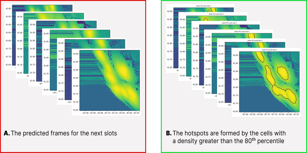
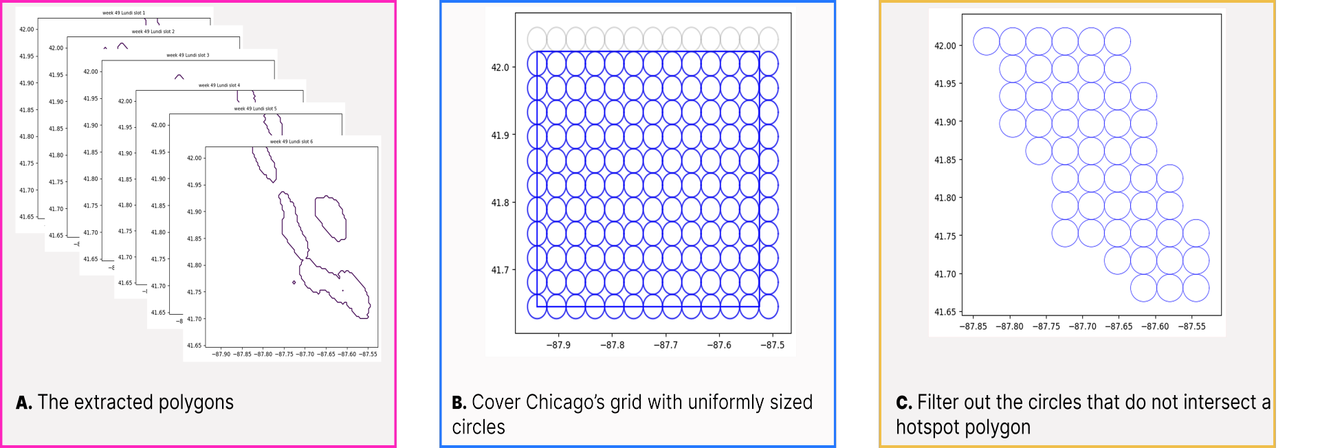
In practice, patrol operations typically focus on a contiguous subset of time slots within a specific day, denoted (for example, a work shift). That is, algorithm 4 converts predicted heatmaps into deployment locations by detecting high-risk cells within each time slot using a -th percentile threshold. Following [3], we set to the 85%-percentile so that only the top 15% of predicted intensities are considered hotspots, thereby reducing the impact of outliers. In Step 1 of the algorithm (lines 1–6), each time slot (line 3) is processed by first identifying high-risk cells (line 4), then clustering these cells into contiguous polygons using standard 4-connectivity where neighboring high-risk cells are merged into connected components (line 5) (Figures 4.B, 5.A), and finally merging the resulting polygons into the set allPolygons (line 6). Next, in Step 2 (line 7), a uniform grid of circles is generated over the city grid to form allCircles (Figure 5.B). In Step 3 (lines 8–13), every circle in allCircles (line 9) is examined against each polygon in allPolygons (line 10), and if the circle satisfies the IntersectsOrInside condition (line 11), it is appended to the list validCircles (line 12) and the inner loop is exited (line 13) (Figure 5.C). Finally, in Step 4, for each valid circle (line 15) the algorithm computes the time-slot-specific risk by summing the risk values of all cells completely inside the circle for each slot (line 18). The circle’s center, paired with its list of per-slot risks, is then added to locations (line 20), producing as output a set of pairs , where tsRisk contains a risk value for every time slot in .
5 Constraint Programming Formulation
Building on the refined set of high-risk deployment locations identified via the ML-to-CP step, we formulate a vehicle routing problem (VRP) to optimize patrol unit deployment. The problem is defined on a directed graph , where represents locations (with location denoting the depot) and defines admissible travel arcs. The subset corresponds to the deployment locations selected by ML-to-CP. The planning horizon is discretized into slots, , each of duration slot_length. Patrol routes must be completed within a maximum allowable time maxT.
We consider a set of patrol units (vehicles), Each location has a service time . Each deployment location has a time-varying risk value for each slot . Travel times between locations and are given by .
For each vehicle , we introduce a variable indicating how many locations that vehicle visits (including its first position). We also allow each patrol to start at any location at time .
The decision variables can be summarized as follows:
-
: the -th location visited by vehicle .
-
: arrival, departure, and waiting times at the -th location of vehicle .
-
: time slot during which vehicle services its -th location ( indicates either the depot or an unused slot).
-
: total number of visited locations by vehicle .
The key constraints are as follows:
-
Vehicles may begin at any location at time :
-
Beyond the route length of a vehicle (i.e. ), we force the following decision variables to be :
-
No vehicle returns to the depot prematurely:
-
A vehicle must complete its service time and any waiting time before departing:
-
The arrival time at the next location depends on the departure time from the current one plus travel time:
-
If the location is a deployment location, determine the slot by (Mapping Arrival Times to Slots):
-
Prevent two vehicles from serving the same deployment location simultaneously:
Objective Function.
The goal is to maximize the overall “risk coverage” achieved by assigning patrol vehicles to specific high-risk locations at times when risks are high. Specifically, each visit to a deployment location in time slot contributes to the objective. Because vehicles follow routes and visit multiple locations sequentially, the objective function
sums the risk values for every pair across all vehicles and all visited points . In other words, whenever vehicle visits location during slot , that location’s time-dependent risk is accrued toward the total. Hence, the model is driven to schedule patrol units so that the highest-risk locations are visited at the most impactful time slots, thereby maximizing the sum of all risk covered during the planning horizon.
6 Results
In this section, we present and discuss the training of our XLearn model and the subsequent results obtained from both validation and testing. We further demonstrate the effectiveness of the proposed strategy through ICON loop simulations.
6.1 Training XLearn
The core of our ML component is the XLearn model, which builds on the PredRNN++ architecture [27]. We use the publicly available PredRNN++ implementation provided in the OpenSTL repository444https://github.com/chengtan9907/OpenSTL. Our experiments adopt the default architecture and training configuration, except for the number of recurrent layers, which we increase from four to six by adjusting the hidden layer structure. All other hyperparameters – including convolutional filter size, patch size, learning rate, batch size, and the scheduled sampling schedule – remain unchanged. The model is trained with cell-wise Mean-Squared Error.
Data Preparation and Setup
As mentioned earlier, we evaluated XLearn on the City of Chicago Crime Dataset [24], focusing on reported incidents from 2023. After cleaning, the processed data amounted to records, from which we retained only latitude, longitude, and time as relevant features. Following Section 3, World-to-ML transformed these raw crime observations into a sequence of quantile-based matrices, . With one year split into weeks, days per week, and time slots of half an hour per day, we obtained matrices, each encoding the spatial distribution of crime risk at a specific slot.
Model Training
We implemented applyXLearn (Algorithm 3) to form training pairs . Afterwards, an 80%–15%–5% split was applied for training, validation, and testing, respectively. Various input-sequence lengths were tested, and a good configuration was found at . The output-sequence length corresponds to a single prediction step (i.e., forecasting the upcoming time slot of the next day).
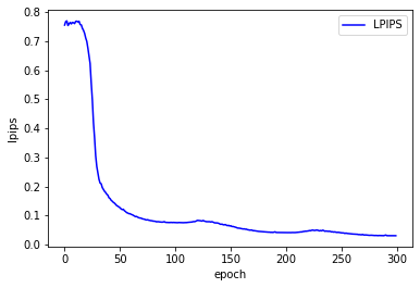
We trained for epochs on an HPC equipped with an NVIDIA A100-GPU, running CUDA 12.2. The GPU had a maximum memory capacity of MiB. Figure 7A plots the training and validation loss curves over epochs. Both curves show steady progress and minimal overfitting.
We assessed model accuracy and fidelity using four widely adopted metrics:
-
Mean Squared Error (MSE) measures the average squared differences between predictions and ground-truth data;
-
Peak Signal-to-Noise Ratio (PSNR) [13], expressed in decibels (dB), quantifies reconstruction fidelity (higher values, typically – dB, denote better quality);
-
Structural Similarity Index (SSIM) [28], which evaluates structural alignment between images on a scale of to ( corresponds to perfect match);
-
Learned Perceptual Image Patch Similarity (LPIPS) [29], a deep-learning metric scored between and , where lower values indicate greater perceptual resemblance in feature space ( for identical images).
Figures 7B–7D depict the PSNR, SSIM, and LPIPS metrics over training epochs. Our best validation metrics reached:
-
, indicating a high-fidelity reconstruction,
-
, reflecting strong structural alignment with the ground truth,
-
, suggesting high perceptual similarity.
On the held-out test set, the model consistently achieved: , indicating that XLearn generalizes well: it preserves essential structure (SSIM), yields visually coherent predictions (PSNR), and remains perceptually faithful (LPIPS) (Figure 6).


Overall, these results confirm that the PredRNN++ XLearn effectively captures spatial-temporal crime patterns, producing robust and high-quality forecasts that are well-suited for guiding subsequent patrol route optimization.
6.2 Simulating the ICON loop
We conducted our simulations on a computer equipped with a 12th Gen Intel® CoreTM i7-12700H processor ( GHz), GB RAM, and a 64-bit Windows operating system. We set a fixed service time of 20 minutes per location. Travel distances were computed using the OSMnx Python library [2], assuming a constant travel speed of km/h.
To maintain operational feasibility, we set the radius of each deployment location circle to . This radius ensures that traversing the circle’s perimeter () takes approximately 12.6 minutes, fitting comfortably within the 20-minute service duration. Hence, a radius allows sufficient time to patrol the perimeter fully, make strategic movements, or handle additional points of interest within the deployment area. By contrast, increasing the radius to or would expand the perimeter to roughly or , complicating thorough coverage of the deployment area.
We performed simulations using week of (unseen during training) from the Chicago Crime Dataset [24]. Each cycle of the ICON loop spans three hours, subdivided into six consecutive 30-minute time slots (so for the full day, but only 6 slots per cycle). Thus, each day includes cycles, and the full simulation week consists of cycles. After each cycle, simulation time is advanced by exactly 3 hours. The vehicle routing problem is solved for each individual 3-hour cycle. We examined three distinct approaches for crime deterrence:
Predicted Hotspots.
This strategy combines forecasting and patrol planning in three main steps:
-
1.
Forecasting crime risk. Each day is divided into 48 time slots of 30 minutes. For any 3-hour deployment cycle, we focus on a window of 6 consecutive slots . For each slot , the World-to-ML function retrieves the historical sequence of crime-density matrices over the previous days. These sequences are passed to the applyXLearn function, which, using a pre-trained model (trainFlag = false), generates forecasts representing predicted crime risk in each time slot.
-
2.
Identifying deployment locations. The predicted risk matrices are then processed by the ML-to-CP module. This step transforms each heatmap into a set of actionable patrol locations by applying a quantile-based threshold (e.g., top 15% of risk values) and clustering nearby high-risk cells. The result is a list of circular zones likely to contain high-risk activity, suitable for patrol deployment.
-
3.
Optimizing patrol routes. Using operational parameters provided by World-to-CP – such as the number of available patrol units and maximum route duration – the applyXsolve function builds a constraint network incorporating the selected deployment zones. The CP solver then computes patrol routes that maximize total crime risk coverage within the cycle’s 3-hour window.
Historical Hotspots.
This alternative approach replaces forecasting with a simple aggregation of past observations:
-
1.
Averaging past crime patterns. For each of the six 30-minute slots in the 3-hour deployment window , we collect the corresponding historical matrices from the previous days. By computing the element-wise average across days, we obtain , which serve as estimated crime-risk distributions for each slot.
-
2.
Extracting hotspot locations. These averaged heatmaps are then passed to the ML-to-CP module, which applies the same quantile-based thresholding and clustering procedure as in the predicted hotspot approach. The result is a set of patrol deployment zones derived from historical trends.
-
3.
Route optimization. Given these deployment locations and the real-world constraints provided by World-to-CP, the CP solver computes optimized patrol routes to maximize the total historical risk covered during the cycle.
Constraint Satisfaction.
This approach serves as a baseline that prioritizes feasibility over risk-based optimization:
-
1.
Random selection of locations: A set of approximately circles is selected randomly. This quantity mirrors the scale of candidate locations derived by the other approaches. Crucially, these circles are chosen without reference to any crime data, resulting in an arbitrary spatial distribution.
-
2.
No risk prioritization: Patrol routes are computed among these randomly placed circles, adhering only to basic feasibility constraints. Consequently, this approach provides a baseline for comparison, illustrating the effect of disregarding crime-intensity indicators entirely.
Once patrol routes are fixed for a 3-hour cycle, the deterrence rate is determined as follows:
For each vehicle , let be the set of points visited during that cycle. Define the number of deterred crimes for vehicle , denoted , as
where is the distance from crime cr to point , and is the time at which crime cr occurred. Thus, for each visited point , we count all crimes within the patrol’s deployment circle of radius that fall between arrival and departure times.
The overall deterrence rate for the cycle is then computed as
where is the total number of crimes in the study area during the same 3-hour window. This process is repeated for each cycle in our evaluation, and the final hit rate is the mean across all cycles.
| Scenarios | Predicted Hotspots | Historical Hotspots | Constraint Satisfaction |
| 2 patrols | 8 | 3 | 0.1 |
| 4 patrols | 14 | 6 | 0.2 |
| 6 patrols | 19 | 8 | 0.3 |
| 8 patrols | 24 | 10 | 0.4 |
| 10 patrols | 26 | 13 | 0.7 |
Table 1 shows the average hit rates (i.e., the fraction of crimes deterred) for each approach when varying the number of patrol units. The Predicted Hotspots method consistently achieves the highest hit rates, highlighting the benefits of using forecasts to guide where patrols should be deployed. Even with only two patrols, this approach yields a deterrence rate of about , which further increases to when ten patrols are used. This improvement illustrates how forecasting-based route assignments can be scaled up to maintain significant coverage in larger forces.
The Historical Hotspots method performs moderately well, with hit rates surpassing those of the random baseline but trailing behind the predicted hotspot approach. As the number of patrols increases, however, the historical method still benefits from having more units to cover broader areas.
The Constraint Satisfaction approach serves as a baseline. Due to its purely random location selection and route generation, the resulting hit rates are understandably quite low (ranging from to ), underscoring the importance of using forecasts in patrol routing. Despite having a comparable number of potential deployment circles to the other approaches, the absence of risk prioritization substantially diminishes this method’s effectiveness.
6.3 Discussion: Closing the ICON loop
The results confirm that forecasts generated by PredRNN++ can guide the CP-based patrol-routing model to cover significantly more risk than baseline strategies, validating the usefulness of the ML-to-CP channel within each ICON loop cycle. However, in the present work, the CP-to-ML direction (Figure 1) was not exploited, meaning that the information flow remains one-way: forecasts influence patrol plans, but the effectiveness of those plans is not used to improve future predictions. This feedback is critical in operational settings, as patrol deployment can displace or suppress crime and thus modify the spatio-temporal patterns that XLearn must learn in subsequent cycles.
A promising way to activate the CP-to-ML channel is to adopt the Smart Predict then Optimize framework with its surrogate loss SPO+ [9, 22]. The idea is to incorporate feedback from each ICON loop cycle to fine-tune PredRNN++ based on the quality of the patrol plans it enables – measured here by the total risk coverage defined in the objective function.
The procedure may unfold as follows:
-
1.
Observed pass. At the end of a given ICON loop cycle, the most recent crime data is used to construct an observed space–time risk map risk. Solving the CP-based deployment model with this map yields a reference patrol plan. The total risk covered – computed as the sum of across all vehicles and visited locations – is recorded.
-
2.
Feedback. Recall that, earlier in the same cycle, a patrol plan was already computed using the predicted map risk produced by PredRNN++. The difference in total risk coverage between the reference plan (based on observed data) and the forecast-based plan can be interpreted as a loss. SPO+ can then be used to convert this gap into a gradient, which is backpropagated to fine-tune PredRNN++, encouraging it to generate forecasts that lead to more effective patrol deployments in future cycles.
This decision-aware fine-tuning requires only one additional solve per cycle – on the observed risk map – and can be performed offline without disrupting operations. It effectively closes the ICON loop by turning each patrol deployment into both a consequence of current forecasts and a source of supervision for future predictions. By doing so, the learning objective of the ML module is aligned with the operational goal of maximizing total risk coverage throughout the planning horizon.
7 Conclusion
This paper introduced a data-driven framework that integrates predictive modeling and constraint-based optimization to improve the efficiency of police patrol deployments. By using a PredRNN++ approach to generate spatiotemporal crime forecasts, our system anticipates evolving crime risks. These forecasts are then mapped into actionable hotspots via quantile transformations and geometric filtering, before being passed to the constraint programming component for patrol route optimization.
Results from simulations on the Chicago Crime Dataset confirm that prediction-informed routing policies achieve higher hit rates compared to methods relying on static historical data or random deployments. Future work will focus on extending the model to account for multi-criteria decision-making, incorporating additional data sources (e.g., demographic or environmental factors), and exploring more sophisticated forecasting architectures. Overall, our findings demonstrate the promise of tightly coupling machine learning and constraint programming for proactive, effective crime prevention strategies.
References
- [1] Christian Bessiere, Luc De Raedt, Tias Guns, Lars Kotthoff, Mirco Nanni, Siegfried Nijssen, Barry O’Sullivan, Anastasia Paparrizou, Dino Pedreschi, and Helmut Simonis. The inductive constraint programming loop. IEEE Intelligent Systems, 32(5):44–52, 2017. doi:10.1109/MIS.2017.3711637.
- [2] Geoff Boeing. Osmnx: New methods for acquiring, constructing, analyzing, and visualizing complex street networks. Computers, Environment and Urban Systems, 65:126–139, 2017. doi:10.1016/j.compenvurbsys.2017.05.004.
- [3] Kate J Bowers, Shane D Johnson, and Ken Pease. Prospective hot-spotting: the future of crime mapping? British journal of criminology, 44(5):641–658, 2004.
- [4] Eugenio Cesario, Paolo Lindia, and Andrea Vinci. Multi-density crime predictor: an approach to forecast criminal activities in multi-density crime hotspots. Journal of Big Data, 11(1):75, 2024. doi:10.1186/S40537-024-00935-4.
- [5] Spencer Chainey, Lisa Tompson, and Sebastian Uhlig. The utility of hotspot mapping for predicting spatial patterns of crime. Security journal, 21:4–28, 2008.
- [6] Huanfa Chen, T. Cheng, and Sarah Wise. Designing daily patrol routes for policing based on ant colony algorithm. ISPRS Annals of Photogrammetry, Remote Sensing and Spatial Information Sciences, II-4/W2:103–109, July 2015. doi:10.5194/isprsannals-II-4-W2-103-2015.
- [7] Huanfa Chen, T. Cheng, and Xinyue ye. Designing efficient and balanced police patrol districts on an urban street network. International Journal of Geographical Information Science, 33:1–22, October 2018. doi:10.1080/13658816.2018.1525493.
- [8] Maite Dewinter, Christophe Vandeviver, Tom Vander Beken, and Frank Witlox. Analysing the police patrol routing problem: A review. ISPRS Int. J. Geo-Information, 9(3):157, 2020. doi:10.3390/ijgi9030157.
- [9] Adam N. Elmachtoub and Paul Grigas. Smart “Predict, then optimize”. Manag. Sci., 68(1):9–26, 2022. doi:10.1287/MNSC.2020.3922.
- [10] Xinge Han, Xiaofeng Hu, Huanggang Wu, Bing Shen, and Jiansong Wu. Risk prediction of theft crimes in urban communities: An integrated model of lstm and st-gcn. IEE ACCESS, 8:217222–217230, 2020. doi:10.1109/ACCESS.2020.3041924.
- [11] Timothy Hart and Paul Zandbergen. Kernel density estimation and hotspot mapping: Examining the influence of interpolation method, grid cell size, and bandwidth on crime forecasting. Policing: An International Journal of Police Strategies & Management, 37(2):305–323, 2014.
- [12] Corey D Holmes, Christian Orji, and Chris Papesh. Geospatial temporal crime prediction using convolution and lstm neural networks: Enhancing the las vegas cardiff model. SMU Data Science Review, 8(2):3, 2024.
- [13] Alain Hore and Djemel Ziou. Image quality metrics: PSNR vs. SSIM. In 2010 20th international conference on pattern recognition, pages 2366–2369. IEEE, 2010.
- [14] Maja Kalinic and Jukka Matthias Krisp. Kernel density estimation (kde) vs. hot-spot analysis–detecting criminal hot spots in the city of san francisco. In The 21st AGILE International Conference on Geographic Information Science, Lund, Sweden, 2018.
- [15] Jintao Ke, Hongyu Zheng, Hai Yang, and Xiqun Michael Chen. Short-term forecasting of passenger demand under on-demand ride services: A spatio-temporal deep learning approach. Transportation research part C: Emerging technologies, 85:591–608, 2017.
- [16] Dongyeon Kim, Yejin Kan, YooJin Aum, Wanhee Lee, and Gangman Yi. Hotspots-based patrol route optimization algorithm for smart policing. Heliyon, 9(10):e20931, 2023. doi:10.1016/j.heliyon.2023.e20931.
- [17] Yunfeng Kong, Yanfang Zhu, and Yujing Wang. A center-based modeling approach to solve the districting problem. International Journal of Geographical Information Science, 33(2):368–384, 2019. doi:10.1080/13658816.2018.1474472.
- [18] Zhonghang Li, Chao Huang, Lianghao Xia, Yong Xu, and Jian Pei. Spatial-temporal hypergraph self-supervised learning for crime prediction. In 2022 IEEE 38th international conference on data engineering (ICDE), pages 2984–2996. IEEE, 2022. doi:10.1109/ICDE53745.2022.00269.
- [19] Ying-Lung Lin, Meng-Feng Yen, and Liang-Chih Yu. Grid-based crime prediction using geographical features. ISPRS International Journal of Geo-Information, 7(8):298, 2018. doi:10.3390/IJGI7080298.
- [20] He Luo, Peng Zhang, Jiajie Wang, Guoqiang Wang, and Fanhe Meng. Traffic patrolling routing problem with drones in an urban road system. Sensors, 19(23):5164, 2019. doi:10.3390/s19235164.
- [21] X. Lv, Changfeng Jing, Yi Wang, and S. Jin. A deep neural network for spatiotemporal prediction of theft crimes. The International Archives of the Photogrammetry, Remote Sensing and Spatial Information Sciences, XLVIII-3/W2-2022:35–41, October 2022. doi:10.5194/isprs-archives-XLVIII-3-W2-2022-35-2022.
- [22] Jayanta Mandi, Emir Demirovic, Peter J. Stuckey, and Tias Guns. Smart predict-and-optimize for hard combinatorial optimization problems. In The Thirty-Fourth AAAI Conference on Artificial Intelligence, AAAI 2020, pages 1603–1610. AAAI Press, 2020. doi:10.1609/AAAI.V34I02.5521.
- [23] Fatemeh Mousapour, Rajan Batta, and Jose L. Walteros. On the development and analysis of a comprehensive police patrolling model. EURO Journal on Transportation and Logistics, 14:100153, 2025. doi:10.1016/j.ejtl.2025.100153.
- [24] Data Portal. City of chicago. URL: https://data.cityofchicago.org/Public-Safety/Crimes-2023/xguy-4ndq/about_data.
- [25] Jerry Ratcliffe. Intelligence-led policing. Willan Publishing, 2008.
- [26] Sukanya Samanta, Goutam Sen, and Soumya Kanti Ghosh. A literature review on police patrolling problems. Annals of Operations Research, 316(2):1063–1106, 2022. doi:10.1007/S10479-021-04167-0.
- [27] Yunbo Wang, Zhifeng Gao, Mingsheng Long, Jianmin Wang, and S Yu Philip. Predrnn++: Towards a resolution of the deep-in-time dilemma in spatiotemporal predictive learning. In International conference on machine learning, pages 5123–5132. PMLR, 2018.
- [28] Zhou Wang, Alan C Bovik, Hamid R Sheikh, and Eero P Simoncelli. Image quality assessment: from error visibility to structural similarity. IEEE transactions on image processing, 13(4):600–612, 2004. doi:10.1109/TIP.2003.819861.
- [29] Richard Zhang, Phillip Isola, Alexei A Efros, Eli Shechtman, and Oliver Wang. The unreasonable effectiveness of deep features as a perceptual metric. In Proceedings of the IEEE conference on computer vision and pattern recognition, pages 586–595, 2018. doi:10.1109/CVPR.2018.00068.
- [30] Di Zhu, Ninghua Wang, Lun Wu, and Yu Liu. Street as a big geo-data assembly and analysis unit in urban studies: A case study using beijing taxi data. Applied Geography, 86:152–164, 2017.