Transformer-Based Feature Learning for Algorithm Selection in Combinatorial Optimisation

Abstract
Given a combinatorial optimisation problem, there are typically multiple ways of modelling it for presentation to an automated solver. Choosing the right combination of model and target solver can have a significant impact on the effectiveness of the solving process. The best combination of model and solver can also be instance-dependent: there may not exist a single combination that works best for all instances of the same problem. We consider the task of building machine learning models to automatically select the best combination for a problem instance. Critical to the learning process is to define instance features, which serve as input to the selection model. Our contribution is the automatic learning of instance features directly from the high-level representation of a problem instance using a transformer encoder. We evaluate the performance of our approach using the Essence modelling language via a case study of three problem classes.
Keywords and phrases:
Constraint modelling, algorithm selection, feature extraction, machine learning, transformer architectureCopyright and License:
2012 ACM Subject Classification:
Computing methodologies Artificial intelligenceSupplementary Material:
Software (Source Code): https://github.com/SeppiaBrilla/EFE_project [45]
archived at
Funding:
This work was supported by the European Union’s Justice programme, under GA No 101087342, POLINE (Principles Of Law In National and European VAT), by a scholarship from the Department of Computer Science and Engineering of the University of Bologna, and by UK EPSRC grant EP/V027182/1.Editors:
Maria Garcia de la BandaSeries and Publisher:
1 Introduction
It has long been observed that no single algorithm performs best on all combinatorial optimisation problems, or even on all instances of one problem [48, 34, 31]. This observation gave rise to automated Algorithm Selection (AS), where the aim is to automatically select the best algorithm(s) from a portfolio of algorithms with complementary strengths to solve a given problem instance. AS has been successful in a variety of domains, including Boolean Satisfiability (SAT) [60], Constraint Programming (CP) [44, 18, 5, 6], AI planning [58], and general combinatorial optimisation [35].
An algorithm can be seen as an automated solver (or a parameter configuration of a solver). However, the concept of an algorithm can be extended to include the model (i.e. description) of the problem presented to the solver. There are typically many possible models of a problem, and so high-level constraint modelling languages such as MiniZinc [41] and Essence [23] have been proposed that support the specification of models without commitment to low-level modelling details. Accompanying these languages, modelling toolchains support the automated translation of a higher level representation of a problem to the low-level input supported by automated solvers in different paradigms, such as SAT and CP. These include MiniZinc [41], Conjure [2], and Savile Row [42]. The translation process involves several modelling choices, the combination of which has a significant impact on the performance of the target solver [2].
Adapting AS techniques for the extended context of combining modelling and solving choices is a challenge. AS often relies on training Machine Learning (ML) models to predict the best algorithm(s) for a problem instance based on its features. A good set of input features is critical: they must be informative relative to both the problem instance and the performance landscape of the combination of modelling and solver choices on that instance. One well-known instance feature collection for constraint models is fzn2feat [4], a set of 95 features that can be extracted from a representation of a constraint model written in the FlatZinc modelling language [41]. However, FlatZinc models are low-level representations relative to MiniZinc or Essence models, obtained after modelling choices have been made. Hence, the features extracted are tied to a particular low-level model.
Instead of translating a problem instance into a low-level representation (i.e. FlatZinc) before extracting (fzn2feat) instance features, herein we propose to use a transformer encoder [59] to automatically learn features directly from the high-level representation of the instance. Our approach offers three advantages over the fzn2feat method. First, in contrast to the hand-crafted fzn2feat features, our approach learns instance features automatically from the textual description of a problem instance. Second, fzn2feat relies on a low-level problem representation in FlatZinc, while our approach works directly on a high-level representation, which can offer more information for the task of choosing the best combination of model and solver. Third, as shown empirically, the proposed features, once learned, are computationally cheaper to extract. We demonstrate our approach using the Essence constraint modelling pipeline via three case studies that present disparate modelling and solving challenges: Car Sequencing [24], Covering Array [30] and Social Golfers [54].
2 Background
2.1 High-level constraint modelling
MiniZinc [41] and Essence [23] are examples of domain-specific modelling languages. Essence supports higher-level concepts in abstract domains, such as functions, relations and sets, and nesting of these (e.g. set of functions). This enables concise problem specification without committing to low-level modelling details. Since abstract domains are not directly represented in typical solvers, they must be refined into commonly supported concrete domains, such as integers, Booleans and collections of these into arrays or sets.
Conjure [2] refines Essence into Essence Prime, a lower level solver-independent constraint modelling language [42] similar to MiniZinc. It is able to produce a portfolio of models from a single Essence specification, predominantly by exploring alternative refinement pathways for decision variables with abstract domains. This creates a complex algorithm selection landscape: selecting representations for decision variables with abstract domains is akin to viewpoint selection and it is known to significantly affect solution performance, depending on the problem instances being solved [51]. In Section 5, we present the high-level representations of the three case study problems in Essence and describe the alternative Essence Prime models generated by Conjure.
2.2 Transformer architecture
Neural Networks (NNs) are a powerful ML paradigm, able to learn complex patterns from large datasets without user-defined features [20, 36]. NNs have been successful in a wide range of tasks, including text classification [59]. NNs have multiple layers, each processing the input obtained from the output of the previous layer. The first layer accepts the raw input, and the last produces the final output. Layers are typically followed by activation functions, which introduce non-linearity to facilitate learning [26]. The final activation function projects the output of the last layer onto the desired range (e.g. probabilities for classification models). The most fundamental layer type is the linear layer of neurons, each computing an affine transformation of the input from the previous layer to produce an output. The output features form an -dimensional vector [26].
A specific combination of layers defines its architecture. Over the years, many successful architectures have been presented, each with specific advantages and disadvantages. One of the most famous architectures is the transformer [59], which is specifically designed to address sequential data such as text, more efficiently than traditional recurrent models. The key innovation of the transformer is its attention mechanism, which allows the model to capture relationships between all elements in a sequence simultaneously, rather than processing them sequentially. By considering each input element in the context of all others, rather than in isolation, Transformers have achieved state-of-the-art performance in numerous tasks, including text classification [20, 33].
3 Related Work
ML-based techniques for algorithm selection have been proven effective in many problem domains [60, 58, 38, 34, 31]. The selection of the best algorithm(s) is via the characteristics of the given instance, represented as a feature vector. The goal is to construct predictive machine learning models that maps these instance features to the best algorithm(s), thereby optimising a predefined performance metric (e.g. runtime or solution quality). There is often an additional cost associated with feature extraction, which is taken into account when measuring the performance of an AS approach.
Many ML-based AS tools have been proposed for combinatorial optimisation problems. SATZilla [43, 60, 61] is a state-of-the-art SAT solving system that combines existing SAT solvers in a portfolio and applies AS on top of the constructed portfolio. In addition to adopting various ML techniques (i.e., empirical hardness models for predicting algorithm performance [43, 60], and cost-sensitive pairwise classification approaches for predicting the better algorithms in an algorithm pair [61]), a key success of SATZilla is the development of a comprehensive set of features to characterise SAT instances. SATZilla’s instance features were expertly designed to capture the characteristics of SAT instances, which help ML models to effectively predict SAT solver performance. In fact, in a recent study, a revisited and enhanced version of this SAT feature set has been shown to provide significant improvement to SATZilla’s performance [50], indicating the importance of instance features in AS systems in SAT contexts.
Similarly, in CP contexts, several AS-based solving approaches have been proposed. CPHydra [12] and SUNNY [5, 6, 39] focus on computing an instance-specific schedule of solvers via k-nearest neighbours algorithms. CPHydra uses a small set of 36 features developed by the authors of the work, while SUNNY makes uses of fzn2feat [4], a comprehensive set of features specially designed for characterising constraint problems in flatzinc representations. Recently, highly effective SAT encoding selection approaches for Pseudo-Boolean and linear integer constraints have been developed via a combination of various ML-based AS methods and well-designed instance features [55, 56, 57].
These works highlight the critical role of high-quality instance features in AS approaches. However, designing such features is a challenging task and requires extensive knowledge of the corresponding domains. In response to this challenge, automated feature learning approaches have started to emerge. Recurrent NNs were adopted to learn features directly from the input sequence of item sizes in online bin packing problems, which were then used for selecting among different bin-packing heuristics [3]. In the Travelling Salesman Problem (TSP) domain, a transformer-based architecture was developed to learn instance features directly from the raw TSP instance input [49]. The transformer has also been adopted in a black-box optimisation domain for selecting the best solving algorithm [13]. In this case, the input is the trajectory of the optimisation function. Unlike all the previous work cited, our approach learns features directly from the textual description of any combinatorial optimisation problem instance.
4 Methodology
We assume that we are a given (i) a textual description of a combinatorial optimisation problem instance written in a high-level modelling language (such as Essence) and (ii) a portfolio of algorithms to solve the instance, each a combination of a lower-level model (such as an Essence Prime model) and a solver. Our AS task is to predict with ML the best algorithm for a given instance from this portfolio, defined here as that which solves the given instance in the shortest runtime.
Integrating ML in AS requires: (i) extracting a set of features that accurately characterise the instance, and (ii) using these features to predict the best algorithm in the portfolio for the instance. In this section, we describe our methodology to these two requirements. Our approach is agnostic regarding satisfaction versus optimisation – it just requires that algorithm performance can be measured as a numerical value.
4.1 Transformer-based Neural Network for Feature Learning
We propose to employ an NN that encapsulates a transformer encoder [20] to deal with textual input. This approach has many advantages. First, an NN model can automatically generate the necessary features starting from the raw input. This eliminates the need for handcrafting an effective feature set. Second, transformer encoders such as BERT have been proven to be effective in capturing semantic meaning of textual data, [20], eliminating the need to run a solver to extract the necessary features. For example, since all parameter names are identical across problem instances, we expect the learnt features to capture differences in parameter values. Intuitively, the parameter values of an instance are likely to be correlated with its characteristics, such as problem size, which, in turn, are likely to influence the performance of an algorithm. In principle, our approach could work with any textual input (such as natural language). The advantage of starting from a formal representation (such as Essence) is that it is more structured and precise, while natural language tends to contain ambiguity.
We build two NN models, called B-NN and C-NN and depicted in Figure 1, both of which receive as input the raw text of the instance in tokenized form (where each input word and symbol are transformed into a number).
B-NN Model.
This model learns the best algorithm for a given instance. Learning is modelled as a multi-class classification task where the assigned class is the best algorithm. The final activation function is SoftMax, which generates a probability distribution over all the algorithms in the portfolio, where a higher probability indicates a higher likelihood to be the best. SoftMax activation is well suited to associating the highest probability to one best algorithm.
C-NN Model.
Learning one best algorithm is restrictive when multiple algorithms perform similarly well. The C-NN model thus learns the competitiveness of the algorithms in the portfolio. We consider an algorithm competitive if it solves an instance in under ten seconds or less than double the time taken by the best algorithm for that instance. Hence, multiple algorithms may be deemed competitive. We propose to model learning as a multi-label classification task where each algorithm is associated with a competitiveness fraction. The final activation function is Sigmoid, which yields a probability per algorithm, and is well suited to our purpose: there could be multiple equally competitive algorithms and the competitiveness probability of one algorithm is uncorrelated with that of the others. We refrain from using SoftMax activation with the top competitive algorithms, as the number of competitive algorithms is not fixed. Imposing a fixed value of may constrain the model when the actual number of competitive algorithms exceeds , and may lead to incorrect representations when it is fewer than .
The two models share the same architecture, differing in their final activation function. The probability values in their output will be part of the extracted features for AS (as described in Section 4.2). The common part of the models (referred to as core) is composed of three components: (i) Transformer Encoder, (ii) Feature Elaborator, and (iii) Output Layer. Increasing the depth of the network by incorporating multiple layers with different objectives enhances the learning process [53].
Transformer Encoder.
Transformer Encoder transforms input instance text into a feature vector describing its semantic meaning without any pre-processing. The encoder is based on the BERT-base-uncased [20] architecture and shares hyper-parameters with the original except an increased input size (2048 tokens instead of 512) to support large textual input. Our choice of architecture is motivated by several factors. First, it has been successfully applied to classification tasks [46], making it a strong candidate for our purposes. Second, since we do not employ a pre-trained model, BERT shares the same architecture as RoBERTa [40]. Third, although architectures such as Longformer [9] offer a larger context window and more parameters, they are also more computationally expensive, and our preliminary experiments did not demonstrate any clear advantage.
Feature Elaborator.
Feature Elaborator passes the feature vector from the Transformer Encoder through two layers and the corresponding activation functions to project the features into the desired dimension. The Feature Layer is a linear layer that condenses the feature vector, mitigating the risk of dimensionality issues in subsequent non-neural ML applications (curse of dimensionality) [17]. Tanh activation replicates the last activation function of the BERT Transformer Encoder on the reduced feature vector. Its output will be part of the extracted features for AS (as described in Section 4.2). Post-Feature Layer is a linear layer that up-projects the feature vector, allowing the model to further elaborate the features avoiding underfitting [47]. Relu activation introduces non-linearity on the up-projected vector to facilitate learning.
Output Layer.
Output Layer operates on the features to predict a floating point score per algorithm in the portfolio (referred to as Raw output). The final activation functions of B-NN and C-NN transform raw output into probabilities to better interpret it.
4.2 Algorithm Selection Using the Learnt Features
To address the second requirement of our ML-based AS we propose two approaches: integrating feature learning and AS within a single NN model (referred to as fully neural), or exploiting an external ML-based AS algorithm using the extracted features (referred to as hybrid). While the first approach seems natural and more straightforward, the latter allows exploiting state-of-the-art AS tools and experimenting with alternative AS strategies.
Once the NN models are trained, we can use B-NN as a fully neural approach to predict the best algorithm by using the probability values in the output as features and picking the algorithm associated with the highest probability. For the hybrid approach, we extract features from each NN model by combining the probability values in the output with the output of Tanh in a single feature vector. We have observed in a preliminary study that the models trained using only the Tanh output misclassified some instances with a prediction that was not deemed as competitive by the NN. We thus combined it with the probability output to limit this type of error. The combined feature vector integrates the encoder-derived semantic representation with informative prediction, as we will show in Section 6.5. We refer to such combined feature vectors as b-NN and c-NN features (Fig. 1).
As an external ML-based AS algorithm, we consider both the state-of-the-art Autofolio [38] and a simpler alternative. Autofolio can perform both classification and regression and can be tuned via SMAC [37]. The tuning process can choose between random forest for classification, random forest for regression, and XGboost [14], as well as refine the sets of hyper-parameters via Bayesian optimisation. Each configuration is evaluated using 10-cross-fold evaluation.
A simpler alternative is clustering, motivated by its success in AS [8] and the spatial characteristics of transformer encoder embeddings [27]: semantically similar instances are represented by similar vectors. We cluster the instances using K-means [1] based on their similarities and assign to each cluster the algorithm with the lowest total runtime on the cluster instances. For optimisation, we pre-define a set of hyper-parameter configurations, each evaluated by fitting a model on the training data and scoring its performance on the evaluation data. The score is calculated by assigning validation instances to their respective clusters and evaluating them with the corresponding algorithm. The configuration with the lowest total score is selected as the optimal. At test time, an unseen instance is assigned to a cluster based on the best-fit configuration and the cluster’s algorithm is applied as the best algorithm.
In summary, we have five ML-based AS approaches: fully neural B-NN and four hybrids (b-NN,A), (b-NN,K), (c-NN,A), (c-NN,K), where A, and K denote Autofolio and K-means.
5 Case Studies
We evaluate our methodology using the Essence constraint modelling pipeline via three well-known, challenging problems: Car Sequencing, Covering Array and Social Golfers. In the following sections, we first present an Essence model for each problem, followed by a description of its algorithm portfolio, which consists of various combinations of an Essence Prime model (obtained from Conjure) and a solver. To establish suitability for AS, we then show for each problem that the algorithms in the portfolio have complementary performance on the chosen instance set, i.e. there is no dominating algorithm.
We use instances from [52], generated using the AutoIG framework [19], which systematically varies problem parameters to produce diverse and challenging instance set. Our selection of instances varies in domain size and number of variables, covering a wide range of problem sizes (small, medium, and large) and levels of difficulty. All models and instance sets are publicly available in the Essence Catalogue [16] and in the supplementary repository. 111 https://github.com/SeppiaBrilla/EFE_project/
5.1 Problem Description in Essence and Instance Set
Car Sequencing.
Car Sequencing [22] involves scheduling the production of a set of cars, each potentially requiring different optional features. The production line is divided into stations, each responsible for installing a particular option (e.g., air conditioning, sunroofs). Figure 2(a) shows the parameter and decision variable declarations in an Essence model. It defines three integer parameters: n_cars, n_classes, and n_options, from which domains Slots, Class, and Option are derived. Further parameters refine the problem: quantity, mapping each class to the number of cars required; maxcars, mapping each option to the maximum number of cars allowed in any consecutive block; blksize, a function mapping each option to the size of each consecutive block; and usage, a relation indicating which classes require which options. A decision variable with an abstract domain, car, maps from production slots to classes.
The problem contains a single top level constraint. This constraint uses a sliding-window mechanism to control the distribution of options along the car sequence. For each option, it defines a window of consecutive car slots whose length is the sum of the maximum allowed cars with that option and an additional block size delta. Within every such window, the total number of cars requiring the option must not exceed the allowed maximum. This ensures that the usage of each option is evenly distributed, preventing any clustering that could overload production capabilities.
We use 10,214 car sequencing instances.
Covering Array.
Covering Array [30] originates from hardware design. A covering array CA of size is a array over in which every -way combination of row indices and values appears in at least one column. The smallest such is called the covering array number, CAN. We use the decision version of the problem (Figure 2(b)). The input parameters of the model are: t, the strength, k, the rows, g the array’s values domain, b the number of columns of the covering array. The decision variable is CA: an integer-indexed matrix of integer values in the range 1 to g.
The first constraint in this model requires that for every strictly increasing sequence of rows, every possible combination of values (from the available) is represented in at least one column of the matrix CA. This guarantees that the matrix forms a covering array of strength . The remaining two constraints are for symmetry breaking.
We use 2,236 instances for this problem.
Social Golfers.
Social Golfers [54] involves scheduling golfers in groups of size for weeks, such that no pair of golfers meets more than once. Figure 2(c) shows the parameter and decision variable in an Essence model of the problem. An unnamed type, Golfers, represents all the golfers in the schedule, with size . The decision variable, sched, is a set of partitions, each corresponding to a week’s grouping of golfers.
The only constraint in this model is that of socialisation: it ensures that any two distinct golfers are paired together in the same group in at most one week. For every pair, it sums a Boolean indicator (converted to an integer) across all weeks, with each indicator signalling whether the pair played together in that week. The total for each pair is constrained to be no more than one, ensuring that no pair of golfers is scheduled to play together more than once over the course of the weeks.
We use 1,039 instances for this problem.
5.2 Combinations of Essence Prime Models and Solvers
We use Conjure in portfolio mode to generate up to four Essence Prime models from a single Essence specification, exploring different ways to represent variables and constraints. Key model variations for each problem are summarised below. We then combine the various Essence Prime models with four solvers to create a diverse set of algorithms that may perform well on different subsets of instances.
Car Sequencing.
Car Sequencing has three models based on two representations for the car decision variable and the usage parameter. The car variable can be represented as either a one-dimensional array of integers or a two-dimensional Boolean array, while the usage parameter can be either a Boolean array or a set of tuples. Model uses a one-dimensional array for car and a set of tuples with a table constraint for usage. Model uses a one-dimensional array for car with a Boolean array for usage and the element constraint. Model uses a two-dimensional Boolean array for car and a set of tuples with a table constraint for usage.
Covering Array.
Covering Array has one model because the problem is expressed with a single matrix decision variable, and matrix variables map directly to Essence Prime. The constraints likewise do not permit additional variations.
Social Golfers.
Social Golfers has four models offering different matrix-based encodings of the weekly partitions. Model uses a single 3D matrix indexed by , where each entry is an integer indicating which golfer is in a particular part of the partition for a particular group and week. uses a 3D Boolean matrix, indexed by weeks, groups, and golfers, to indicate whether a given golfer is in a specific part of the partition. splits the partitioning into multiple matrices, capturing information such as the number of parts, which golfer goes into each position, and how many slots are used in each group. By breaking down the partition into several matrices, this approach can exploit different constraint formulations within the same overall representation. combines two matrix encodings: one stores explicit integer assignments for each slot and another tracks membership via Booleans.
Solvers.
5.3 Algorithm Complementarity
We analyse the portfolio of algorithms employed for each problem and assess the potential benefits of applying AS. In Section 4, we defined the best algorithm in terms of shortest runtime. In practice, we often impose a cut-off time on every algorithm. When an algorithm fails to solve an instance within the cut-off, we penalise the run using the PAR10 (Penalised Average Runtime) metric [38], where the runtime of a failed run is recorded as times the cut-off time.
All experiments were conducted on a computational setup equipped with an AMD EPYC 7763 CPU. Each algorithm was allocated a single CPU core with a one-hour cut-off per instance. As baseline, we will use the Single Best Solver (SBS) algorithm, defined as the algorithm with the lowest PAR10 score in the whole instance set, and the Virtual Best Solver (VBS), a theoretical construct representing the optimal algorithm selector that always identifies the best algorithm for each instance.
Car Sequencing.
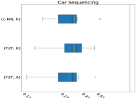
Car Sequencing uses a portfolio of 12 algorithms derived from the combination of three Essence Prime models and four constraint solvers. Figure 3(a) (top) shows the PAR10 scores for these algorithms, evaluated across the entire instance set. A key observation from Figure 3(a) (top) is the lack of a dominant model or solver: there is no algorithm with the same behaviour as VBS, meaning that no algorithm is the “best” on each instance. The algorithms, excluding those involving , which always underperform independently of the solver, exhibit diverse performance characteristics. Notably, the gap between the VBS and the SBS algorithm (-Chuffed) is significant, with the SBS achieving only 0.01% of the VBS’s performance. This underscores the potential for AS to leverage complementary strengths among algorithms. Figure 3(a) (bottom) shows the average competitiveness (as the percentage of the instances where the algorithm is competitive). All algorithms are competitive on some instances, except -CPLEX, which was the worst overall algorithm. It is typically very difficult for an AS method to always select the best algorithm for a given instance. At the same time, this may not always be necessary, as competitive algorithms could also do well on the instance.
We can see that even though -Chuffed appears to be the best overall algorithm in Figure 3(a), it is the winner on a fairly small number of instances according to plot of Figure 4(a). Instead, -CPLEX, -Chuffed and -OR-Tools have significantly higher numbers of instances where they win. These three algorithms, which are also the top three competetive algorithms according to Figure 3(a) (bottom), cover a significant part of the instance space.
Covering Array.
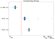
Covering Array has one Essence Prime model, hence four different algorithms combining the model with the four solvers. Figure 3(b) (top) shows PAR10 scores of each algorithm in the full instance set. Contrary to Car Sequencing, for this problem class the gap between SBS and VBS is much smaller. With -Kissat being the SBS, VBS as a fraction of SBS is 0.72. In terms of competitiveness (bottom figure), we can see that -Chuffed and -Kissat are almost always competitive, -CPLEX is competitive around 60% of the time and -OR-Tools roughly 50% of the time. This second view shows a different story from the top figure where -Kissat seems to be the clear winner. This suggests a much more complex instance set where AS could take advantage of the different algorithms.
Even though the gap between SB and VBS is much smaller compared with the Car Sequencing case, Figure 4(b) shows that each algorithm contributes to VBS, even -CPLEX which has the worst PAR10 score. -OR-Tools is the least contributing algorithm while -Chuffed and -Kissat, the main competitive algorithms according to Figure 3(b) (bottom), both contribute similarly to VBS, with -Kissat contributing slightly more than 50% of the time and -Chuffed roughly 45% of the time.
Social Golfers.
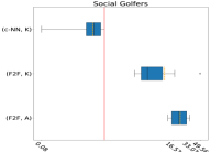
Social Golfers has four Essence Prime models, resulting in sixteen different algorithms in conjunction with the four solvers. The PAR10 scores of Social Golfers (Figure 3(c), top) differ from those of the previous problems: 6 algorithms dominate all the others with similarly bad results. The algorithms including the models and have the best performance when coupled with Chuffed, Kissat and OR-Tools. The same cannot be said for CPLEX because it performs similarly to the other algorithms. The gap between SBS and VBS is in the middle between Car Sequencing and Covering Array since VBS as a fraction of SBS is 0.65. -Chuffed, -Kissat, -OR-Tools, -Chuffed, -Kissat and -OR-Tools are the only competitive algorithms more than 10% of the time (Figure 3(c), bottom). This may seem less than ideal. However, the gap between SBS and VBS shows that whenever -Kissat is not the best algorithm it is worse by a considerable margin, motivating AS.
The participation to VBS, in Figure 4(c), shows that, although -Kissat is the SBS, -Chuffed is the algorithm that contributes by far the most to VBS while -Kissat wins only in a handful of instances. This is a clear indication of the potential of AS for this problem class.
We conclude that each problem in our case study, along with its set of instances and algorithm portfolio, serves as a suitable candidate for evaluating our methodology.
6 Experimental Results
We experimentally evaluate the effectiveness of our five ML-based AS approaches proposed in Section 4: the fully neural B-NN and the four hybrid approaches (b-NN,A), (b-NN,K), (c-NN,A) and (c-NN,K). All source code and data are available in the supplementary repository. 1 The following questions guide the evaluation: (Q1) Is the fully neural approach effective for AS, or is it necessary to split the learning process into two phases (like the hybrids)? (Q2) How do the learnt features compare to the existing fzn2feat features in solving the AS task? (Q3) What is the computational cost of the feature extraction process and its impact on the AS performance? (Q4) Is it beneficial to combine the propabability values in the output of an NN model with the output of Tanh for feature learning?
6.1 Experimental Design
Algorithm Selection Setup.
Each AS approach is evaluated using PAR10 across 10-fold cross validation. In each fold, of the training data serves as a validation set to support neural network training and hyper-parameter optimisation. We use the same computer configuration as in Section 5.3 for the CPU-based experiments, while GPU is used for neural network training and inference, as detailed below. In the hybrid approaches, we make use of K-means and AutoFolio for the AS task. We tested the number of clusters in K-means in the range [2,21] and chose that which resulted in the lowest validation PAR10 score. AutoFolio is an AS framework that offers a tuning mode with its own hyper-parameter configuration space. The tuning is done using the hyper-parameter optimisation tool SMAC [28], which we employ with a single CPU core and a tuning budget of hours.
Neural Network Training.
All NN models are implemented using PyTorch [7] and trained from scratch on a GPU equipped with an NVIDIA A5000 accelerator. The Adam optimiser [32] is employed for all training processes. Model hyper-parameters, including the learning rate, (mini-)batch size, and number of epochs, are selected based on a combination of computational resource constraints and manual experimentation. The final hyper-parameter values are detailed in Appendix A. Cross Entropy is applied in the B-NN models, while Binary Cross Entropy is used in the C-NN models. In addition to the fold mechanism used as a precaution against overfitting, we monitor the validation loss during training and retain the model with the lowest validation loss to further reduce the risk of overfitting.
Normalised PAR10 Score.
Due to the different scales of PAR10 across folds, following the existing AS literature [38], we define the normalised score as , where , and are the PAR10 scores of an AS approach, the VBS, and the SBS on the same fold, respectively. VBS has a score of 0 while SBS has a score of 1. We want to minimise the normalised score. Feature extraction time is included in all PAR10 calculations unless its exclusion is mentioned explicitly. An AS approach is considered effective if its normalised score is less than , i.e., it performs better than SBS – the AS approach without any learning required.
6.2 Fully Neural vs Hybrid Approaches
In this section we address Q1 and compare the fully neural B-NN with its hybrid counter-parts (b-NN,*) and (c-NN,*). Fig. 5 presents the normalised PAR10 scores of the five approaches across 10 folds. Overall, B-NN is generally less competitive than the hybrids. Among the hybrids, (c-NN, K) consistently obtains the best overall performance across the three problems. It is the only one that consistently achieves better performance than SBS. A likely explanation for the underperformance of B-NN is the inherent imbalance of the training data in our multi-class classification setting. Algorithms that excel on only a small subset of instances are under-represented, making them harder to be detected despite their significant impact on the overall PAR10 score. This is confirmed by [11], which demonstrated that treating this task as a pure multi-class classification is generally the least effective approach, since classification accuracy does not account for the actual runtime of each predicted algorithm and thus is not aligned with the final performance metric. The hybrid approaches mitigate this limitation by separating feature learning and AS, and the ML models used in the AS part do take into account performance difference between algorithms, allowing training to be tailored towards the true performance metric PAR10. Finally, (c-NN,K) performs much better than (c-NN,A), despite K-means’ simplicity w.r.t. Autofolio. Our finding illustrates that simpler ML-based AS approaches can be quite effective for certain AS tasks compared with the more sophisticated ones commonly used in the AS literature.
6.3 Comparison with fzn2feat Features
Having established that (c-NN,K) is the best approach for automatically learning instance features, we consider Q2 by comparing our learnt features with fzn2feat (F2F) [4], which were expertly-designed for representing constraint models. Since F2F only works in the low-level constraint representation in FlatZinc, we first need to translate each problem instance into the FlatZinc format [41]. This translation involves choosing a specific combination of an Essence Prime model and a solver. We use conjure’s default model and the Chuffed solver. For each instance, the F2F features are extracted using 2 CPU cores and 8GB RAM, and c-NN feature extraction uses the same GPU-enabled computer as in the training process. The use of different machines is motivated by the slower CPU on the GPU-enabled machine and the observation that fzn2feat runs faster on a CPU-only machine. This setup leverages the hardware characteristics best suited for each computation. While we expect weaker performance on CPU-only systems, emerging consumer hardware with unified memory architectures is likely to narrow this gap. We observe that the memory usage of the c-NN feature extraction process remains under a few GBs; however, in some runs, F2F extraction crashes due to memory limits. In such cases, we revert to SBS as the best algorithm for the corresponding problem instance.
F2F features combined with K-means and Autofolio result in two new AS approaches (F2F,K) and (F2F,A). Fig. 6 shows their normalised PAR10 scores and (c-NN,K)’s on the test set across 10 folds. On Car Sequencing, (c-NN,K) outperforms (F2F,K) on seven out of ten folds. Compared with (F2F,A), (c-NN,K) obtains the best overall median score. The strength of (c-NN,K) is even clearer on the remaining two problems, where it performs significantly better than the F2F-based AS approaches across all folds. In fact, (c-NN,K) is the only one that surpasses SBS. These results further confirm the effectiveness of our proposed learning approach in capturing the semantic properties of high-level constraint instances when compared to the existing low-level F2F features, where essential information about the high-level structure of the problem instance can be lost during translation.
6.4 Feature Extraction Cost
| fold | Car Sequencing | Covering Array | Social Golfers | |||||||||
|---|---|---|---|---|---|---|---|---|---|---|---|---|
| F2F + E | c-NN + E | F2F | c-NN | F2F + E | c-NN + E | F2F | c-NN | F2F + E | c-NN + E | F2F | c-NN | |
| 1 | 132.51 | 300.57 | 127.17 | 300.52 | 23.23 | 14.85 | 19.23 | 14.85 | 1,547.11 | 209.45 | 1,224.51 | 209.44 |
| 2 | 301.97 | 156.22 | 296.69 | 156.17 | 28.60 | 20.99 | 25.00 | 20.99 | 1,163.31 | 268.35 | 848.11 | 268.35 |
| 3 | 273.85 | 212.42 | 268.54 | 212.37 | 26.48 | 15.95 | 22.65 | 15.95 | 518.72 | 234.85 | 199.68 | 234.85 |
| 4 | 229.78 | 179.38 | 224.35 | 179.33 | 25.37 | 18.60 | 21.80 | 18.60 | 1,175.69 | 253.20 | 857.06 | 253.20 |
| 5 | 348.88 | 441.89 | 343.56 | 441.83 | 20.79 | 14.78 | 17.27 | 14.78 | 528.35 | 275.22 | 216.90 | 275.22 |
| 6 | 246.55 | 177.89 | 241.23 | 177.84 | 27.93 | 18.21 | 24.43 | 18.21 | 481.67 | 181.12 | 176.76 | 181.11 |
| 7 | 283.33 | 359.54 | 277.90 | 359.49 | 20.56 | 14.40 | 17.04 | 14.40 | 841.24 | 221.02 | 535.98 | 221.02 |
| 8 | 352.25 | 183.32 | 346.96 | 183.27 | 15.95 | 10.82 | 12.44 | 10.82 | 849.04 | 268.51 | 548.80 | 268.51 |
| 9 | 284.51 | 203.13 | 278.98 | 203.07 | 16.89 | 11.72 | 13.37 | 11.72 | 911.93 | 280.15 | 594.83 | 280.15 |
| 10 | 179.17 | 151.15 | 173.60 | 151.10 | 504.62 | 21.22 | 501.03 | 21.22 | 1,228.29 | 168.23 | 916.30 | 168.23 |
We address Q3 by analysing the computational cost associated with the feature extraction process and its influence on the final AS performance. Table 1 presents average PAR10 scores on the test set of (c-NN,K) and (F2F,K) with (+E) and without feature extraction cost across 10 folds. While the extraction cost of c-NN features is marginal, it is generally higher for F2F, resulting in worse PAR10 scores. On Car Sequencing, feature extraction cost does not affect the ranking between the two approaches: (c-NN,K) performs better than (F2F,K) on a majority of folds (7/10) no matter whether feature extraction cost is included. On Covering Array, the F2F feature extraction cost is smaller in scale and does not impact the relative ranking in AS performance between (c-NN,K) and (F2F,K), as the former is consistently better across all folds. Additionally, even when feature extraction cost is excluded, (F2F,K)’s performance is still worse than SBS across all folds, suggesting that those features are insufficient to capture the semantic properties of this problem. Finally, on Social Golfers, feature extraction cost of F2F significantly negatively impacts the corresponding AS’s overall performance and alter the ranking on 3 folds, while (c-NN,K) achieves better score on the remaining 7 folds no matter what.
| Car Sequencing | Covering Array | Social Golfers | ||||
|---|---|---|---|---|---|---|
| F2F | c-NN | F2F | c-NN | F2F | c-NN | |
| max | 33.68 | 0.33 | 8.96 | 0.26 | 1304.95 | 0.25 |
| min | 0.80 | 0.01 | 3.33 | 0.01 | 0.52 | 0.01 |
| mean | 5.38 | 0.05 | 3.61 | 0.01 | 312.23 | 0.01 |
| median | 6.71 | 0.06 | 3.55 | 0.01 | 271.02 | 0.01 |
Table 2 shows the maximum, minimum, mean, and median extraction cost (in seconds) of the F2F and c-NN features. We observe a better consistency in the values of the c-NN features, which are marginally affected by the instance text size and always negligible. In contrast, the values of the F2F features vary significantly across the three problems, and they are not negligible, especially in the case of Social Golfers.
6.5 Ablation Study
To address Q4, we show in Figure 7 the benefits of combining the NN output probabilities and the Tanh output for feature learning by focusing on the (c-NN,K) approach. Using only the output probabilities (p,K) significantly hinders the learning process and leads to poorer performance compared with using the combined features in (c-NN,K). In contrast, when only the Tanh features are used (t,K), the performance is more comparable with (c-NN,K). Interestingly, for the Covering Array problem, both approaches achieve identical results. However, in the case of Car Sequencing and Social Golfers, both the average and median performance metrics indicate worse outcomes with (t,K) compared to (c-NN,K).
7 Conclusions
We have explored automatic feature learning for algorithm selection on three problems. Our approach employs a transformer encoder to learn instance features directly from a high-level problem description, which are used to predict the best algorithm for solving an instance. Our experiments demonstrate that the learnt features can be effectively used in a diverse set of AS algorithms. In particular, a K-means-based approach performed competitively on all problem classes beating existing state-of-the-art features previously used for AS.
Our results indicate that neural-based feature extraction offers a viable and efficient alternative to traditional methods, with significantly lower computational costs for feature extraction. Furthermore, our results show the importance of extracting features from an high-level instance, especially when the AS task involves selecting the best constraint model as well as a solver.
Our study highlights the potential of ML and automatic feature learning in enhancing algorithm selection for combinatorial problems, paving the way for more adaptive and efficient solving techniques in various application domains.
In future work, we will conduct a more systematic hyper-parameter optimisation of the whole pipeline and explore other types of learning techniques, for instance by representing the problem instances in the form of a graph and using GNNs for feature extraction. We also plan to instantiate our approach on other high-level modelling languages like MiniZinc [41] and CPMpy [25], and adapt it to receive natural language in the input, with the use of LLMs. While challenging due to the the black-box nature of neural network-based approaches, an interesting direction is to analyse the learnt features and be able to explain their semantic meaning.
References
- [1] M. Ahmed, R. Seraj, and S. M. S. Islam. The k-means algorithm: A comprehensive survey and performance evaluation. Electronics, 9(8):1295, 2020.
- [2] Ö. Akgün, A. M Frisch, I. P Gent, C. Jefferson, I. Miguel, and P. Nightingale. Conjure: Automatic generation of constraint models from problem specifications. Artificial Intelligence, 310:103751, 2022. doi:10.1016/J.ARTINT.2022.103751.
- [3] M. Alissa, K. Sim, and E. Hart. Automated algorithm selection: from feature-based to feature-free approaches. Journal of Heuristics, 29(1):1–38, 2023. doi:10.1007/S10732-022-09505-4.
- [4] R. Amadini, M. Gabbrielli, and J. Mauro. An enhanced features extractor for a portfolio of constraint solvers. In Proceedings of the 29th annual ACM symposium on applied computing, pages 1357–1359, 2014.
- [5] R. Amadini, M. Gabbrielli, and J. Mauro. SUNNY: a lazy portfolio approach for constraint solving. Theory and Practice of Logic Programming, 14(4-5):509–524, 2014. doi:10.1017/S1471068414000179.
- [6] R. Amadini, M. Gabbrielli, and J. Mauro. SUNNY-CP: a sequential CP portfolio solver. In Proceedings of the 30th Annual ACM Symposium on Applied Computing, pages 1861–1867, 2015.
- [7] J. Ansel, E. Yang, H. He, N. Gimelshein, A. Jain, M. Voznesensky, B. Bao, P. Bell, D. Berard, E. Burovski, et al. Pytorch 2: Faster machine learning through dynamic python bytecode transformation and graph compilation. In Proceedings of the 29th ACM International Conference on Architectural Support for Programming Languages and Operating Systems, Volume 2, pages 929–947, 2024.
- [8] C. Ansótegui, M. Sellmann, and K. Tierney. Self-configuring cost-sensitive hierarchical clustering with recourse. In Proceedings of the 24th International Conference on Principles and Practice of Constraint Programming, pages 524–534. Springer, 2018.
- [9] I. Beltagy, M. E P.s, and A. Cohan. Longformer: The long-document transformer. arXiv preprint arXiv:2004.05150, 2020.
- [10] A. Biere and M. Fleury. Gimsatul, IsaSAT and Kissat entering the SAT Competition 2022. In Tomas Balyo, Marijn Heule, Markus Iser, Matti Järvisalo, and Martin Suda, editors, Proceedings of SAT Competition 2022 – Solver and Benchmark Descriptions, volume B-2022-1 of Department of Computer Science Series of Publications B, pages 10–11. University of Helsinki, 2022.
- [11] B. Bischl, P. Kerschke, L. Kotthoff, M. Lindauer, Y. Malitsky, A. Fréchette, H. Hoos, F. Hutter, K. Leyton-Brown, K. Tierney, and J. Vanschoren. ASlib: A benchmark library for algorithm selection. Artificial Intelligence, 237:41–58, 2016. doi:10.1016/j.artint.2016.04.003.
- [12] D. Bridge, E. O’Mahony, and B. O’Sullivan. Case-based reasoning for autonomous constraint solving. In Autonomous search, pages 73–95. Springer, 2012. doi:10.1007/978-3-642-21434-9_4.
- [13] G. Cenikj, G. Petelin, and T. Eftimov. Transoptas: Transformer-based algorithm selection for single-objective optimization. In Proceedings of the Genetic and Evolutionary Computation Conference Companion, pages 403–406, 2024.
- [14] T. Chen and C. Guestrin. XGBoost: A scalable tree boosting system. In Proceedings of the 22nd acm sigkdd international conference on knowledge discovery and data mining, pages 785–794, 2016.
- [15] Chuffed Developers. Chuffed, a lazy clause generation solver. https://github.com/chuffed/chuffed. Accessed: 2024-07-05.
- [16] Conjure developers. Essence catalog: A collection of problem specifications in essence. https://github.com/conjure-cp/EssenceCatalog, 2024.
- [17] A. Crespo Márquez. The curse of dimensionality. In Digital Maintenance Management: Guiding Digital Transformation in Maintenance, pages 67–86. Springer, 2022.
- [18] N. Dang. A portfolio-based analysis method for competition results. arXiv preprint arXiv:2205.15414, 2022.
- [19] N. Dang, Özgür Akgün, J. Espasa, I. Miguel, and P. Nightingale. A Framework for Generating Informative Benchmark Instances. In Christine Solnon, editor, Proceedings of the 28th International Conference on Principles and Practice of Constraint Programming, volume 235 of Leibniz International Proceedings in Informatics (LIPIcs), pages 18:1–18:18, Dagstuhl, Germany, 2022. Schloss Dagstuhl – Leibniz-Zentrum für Informatik. doi:10.4230/LIPIcs.CP.2022.18.
- [20] J. Devlin, M. Chang, K. Lee, and K. Toutanova. BERT: Pre-training of deep bidirectional transformers for language understanding. arXiv preprint arXiv:1810.04805, 2018.
- [21] F. Didier, L. Perron, S. Mohajeri, S. A. Gay, T. Cuvelier, and V. Furnon. OR-Tools’ vehicle routing solver: a generic constraint-programming solver with heuristic search for routing problems, 2023.
- [22] M. Dincbas, H. Simonis, and P. Van Hentenryck. Solving the car-sequencing problem in constraint logic programming. In Proceedings of the European Conference on Artificial Intelligence, pages 290–295, 1988.
- [23] A. M. Frisch, W. Harvey, C. Jefferson, B. Martínez-Hernández, and I. Miguel. Essence: A constraint language for specifying combinatorial problems. Constraints, 13(3):268–306, 2008. doi:10.1007/s10601-008-9047-y.
- [24] I. P Gent. Two results on car-sequencing problems. Report University of Strathclyde, APES-02-98, 7, 1998.
- [25] Tias Guns. Increasing modeling language convenience with a universal n-dimensional array, cppy as python-embedded example. In Proceedings of the 18th workshop on Constraint Modelling and Reformulation at CP (Modref 2019), volume 19, 2019.
- [26] K. Gurney. An introduction to neural networks. CRC press, 2018.
- [27] A. Handler. An empirical study of semantic similarity in wordnet and word2vec, 2014.
- [28] F. Hutter, Holger H Hoos, and K. Leyton-Brown. Sequential model-based optimization for general algorithm configuration. In Proceedings of the 5th International Conference on Learning and Intelligent Optimization (LION), pages 507–523. Springer, 2011.
- [29] IBM. Ilog cplex optimization studio: Cplex optimizer. https://www.ibm.com/products/ilog-cplex-optimization-studio/cplex-optimizer, 2022.
- [30] L. Kampel and D. E Simos. A survey on the state of the art of complexity problems for covering arrays. Theoretical Computer Science, 800:107–124, 2019. doi:10.1016/J.TCS.2019.10.019.
- [31] P. Kerschke, H. H Hoos, F. Neumann, and H. Trautmann. Automated algorithm selection: Survey and perspectives. Evolutionary computation, 27(1):3–45, 2019. doi:10.1162/EVCO_A_00242.
- [32] Diederik P Kingma. Adam: A method for stochastic optimization. arXiv preprint arXiv:1412.6980, 2014.
- [33] R. Kora and A. Mohammed. A comprehensive review on transformers models for text classification. In 2023 International Mobile, Intelligent, and Ubiquitous Computing Conference (MIUCC), pages 1–7, 2023. doi:10.1109/MIUCC58832.2023.10278387.
- [34] L. Kotthoff. Algorithm selection for combinatorial search problems: A survey. In Data mining and constraint programming: Foundations of a cross-disciplinary approach, pages 149–190. Springer, 2016. doi:10.1007/978-3-319-50137-6_7.
- [35] L. Kotthoff, P. Kerschke, H. Hoos, and H. Trautmann. Improving the state of the art in inexact TSP solving using per-instance algorithm selection. In LION 9, pages 202–217. Springer, 2015.
- [36] A. Krizhevsky, I. Sutskever, and G. E Hinton. Imagenet classification with deep convolutional neural networks. Advances in Neural Information Processing Systems, 25, 2012.
- [37] M. Lindauer, K. Eggensperger, M. Feurer, A. Biedenkapp, D. Deng, C. B., T. Ruhkopf, R. Sass, and F. Hutter. SMAC3: A versatile bayesian optimization package for hyperparameter optimization. Journal of Machine Learning Research, 23(54):1–9, 2022. URL: http://jmlr.org/papers/v23/21-0888.html.
- [38] M. Lindauer, H. H Hoos, F. H., and T. Schaub. Autofolio: An automatically configured algorithm selector. Journal of Artificial Intelligence Research, 53:745–778, 2015. doi:10.1613/JAIR.4726.
- [39] T. Liu, R. Amadini, M. Gabbrielli, and J. Mauro. sunny-as2: Enhancing SUNNY for algorithm selection. Journal of Artificial Intelligence Research, 72:329–376, 2021. doi:10.1613/JAIR.1.13116.
- [40] Yinhan Liu, Myle Ott, Naman Goyal, Jingfei Du, Mandar Joshi, Danqi Chen, Omer Levy, Mike Lewis, Luke Zettlemoyer, and Veselin Stoyanov. Roberta: A robustly optimized bert pretraining approach. arXiv preprint arXiv:1907.11692, 2019. arXiv:1907.11692.
- [41] N. Nethercote, P. J Stuckey, R. Becket, S. Brand, G. J Duck, and G. Tack. MiniZinc: Towards a standard CP modelling language. In Proceedings of the 13th International Conference on Principles and Practice of Constraint Programming, pages 529–543. Springer, 2007.
- [42] P. Nightingale, Ö. Akgün, I. P Gent, C. Jefferson, I. Miguel, and Patrick Spracklen. Automatically improving constraint models in Savile Row. Artificial Intelligence, 251:35–61, 2017. doi:10.1016/J.ARTINT.2017.07.001.
- [43] E. Nudelman, K. Leyton-Brown, A. Devkar, Y. Shoham, and H. Hoos. SATzilla: An algorithm portfolio for SAT. Solver description, SAT competition, 2004, 2004.
- [44] E. O’Mahony, E. Hebrard, A. Holland, C. Nugent, and B. O’Sullivan. Using case-based reasoning in an algorithm portfolio for constraint solving. In Irish conference on artificial intelligence and cognitive science, pages 210–216, 2008.
- [45] Alessio Pellegrino, Özgür Akgün, Nguyen Dang, Zeynep Kiziltan, and Ian Miguel. EFE repository. Software, version 1.0., swhId: swh:1:dir:0d5708bbc3b0395ddcd80b52bbb6ed8da6ffe252 (visited on 2025-07-22). URL: https://github.com/SeppiaBrilla/EFE_project, doi:10.4230/artifacts.24086.
- [46] R. Qasim, W. H. Bangyal, M. A Alqarni, and A. Ali Almazroi. A fine-tuned bert-based transfer learning approach for text classification. Journal of healthcare engineering, 2022(1):3498123, 2022.
- [47] A. Rangamani, M. Lindegaard, T. GA.ti, and T. A Poggio. Feature learning in deep classifiers through intermediate neural collapse. In International Conference on Machine Learning, pages 28729–28745. PMLR, 2023.
- [48] J. R Rice. The algorithm selection problem. In Advances in computers, volume 15, pages 65–118. Elsevier, 1976. doi:10.1016/S0065-2458(08)60520-3.
- [49] M. V. Seiler, J. Rook, J. Heins, O. L. Preuß, J. Bossek, and H. Trautmann. Using reinforcement learning for per-instance algorithm configuration on the TSP. In IEEE Symposium Series on Computational Intelligence, pages 361–368. IEEE, 2023.
- [50] H. Shavit and H. H Hoos. Revisiting SATZilla features in 2024. In 27th International Conference on Theory and Applications of Satisfiability Testing (SAT 2024), pages 27–1. Schloss Dagstuhl – Leibniz-Zentrum für Informatik, 2024.
- [51] B. M Smith. Modelling. In Foundations of Artificial Intelligence, volume 2, pages 377–406. Elsevier, 2006. doi:10.1016/S1574-6526(06)80015-5.
- [52] P. Spracklen, N. Dang, Ö. Akgün, and I. Miguel. Automated streamliner portfolios for constraint satisfaction problems. Artificial Intelligence, 319:103915, 2023. doi:10.1016/J.ARTINT.2023.103915.
- [53] S. Sun, W. Chen, L. Wang, X. Liu, and T. Liu. On the depth of deep neural networks: A theoretical view. In Proceedings of the AAAI Conference on Artificial Intelligence, volume 30(1), March 2016. doi:10.1609/aaai.v30i1.10243.
- [54] M. Triska and N. Musliu. An effective greedy heuristic for the social golfer problem. Annals of Operations Research, 194(1):413–425, 2012. doi:10.1007/S10479-011-0866-7.
- [55] F. Ulrich-Oltean, P. Nightingale, and J. A. Walker. Selecting SAT encodings for pseudo-boolean and linear integer constraints. In Proceedings of the 28th International Conference on Principles and Practice of Constraint Programming. LIPICS, 2022.
- [56] F. Ulrich-Oltean, P. Nightingale, and J. A. Walker. Learning to select SAT encodings for pseudo-boolean and linear integer constraints. Constraints, 28(3):397–426, 2023. doi:10.1007/S10601-023-09364-1.
- [57] F. Ulrich-Oltean, P. Nightingale, and J. A. Walker. IndiCon: Selecting SAT encodings for individual pseudo-boolean and linear integer constraints. In 2024 IEEE 36th International Conference on Tools with Artificial Intelligence (ICTAI), pages 36–42. IEEE, 2024.
- [58] M. Vallati, L. Chrpa, and D. Kitchin. ASAP: an automatic algorithm selection approach for planning. International Journal on Artificial Intelligence Tools, 23(06):1460032, 2014. doi:10.1142/S021821301460032X.
- [59] A Vaswani. Attention is all you need. Advances in Neural Information Processing, 30, 2017.
- [60] L. Xu, F. Hutter, Holger H Hoos, and K. Leyton-Brown. SATzilla: portfolio-based algorithm selection for SAT. Journal of Artificial Intelligence Research, 32:565–606, 2008. doi:10.1613/JAIR.2490.
- [61] L. Xu, F. Hutter, J. Shen, H. H Hoos, and K. Leyton-Brown. SATzilla2012: improved algorithm selection based on cost-sensitive classification models. Proceedings of SAT Challenge, pages 57–58, 2012.
Appendix A Neural Network Training
A.1 Model Hyper-parameters
For both the B-NN and the C-NN models, we need to set the sizes of the feature and post-feature layers as they are arbitrary and their values can significantly impact both the size of the models and their ability to learn the task effectively. After some manual tuning, we set the size of the feature layer to 100 neurons and the size of the post-feature layer to 200 neurons. These values are large enough to allow a lot of flexibility in the model’s parameters while still being small enough not to cause over-parametrization problems (for the post-feature layer) or issues with the external ASs (for the feature layer).
A.2 B-NN Feature Learning
For each test case, the model was trained using distinct hyper-parameter configurations, including variations in learning rates, the total number of training epochs, and batch sizes. Since we have a limited amount of training data, we observe signs of over-fitting in a number of cases. Therefore, we monitor the validation performance throughout training and retain the model that achieves the best loss value on the validation set.
Figure 8(a) illustrates the evolution of the loss values for both the training and validation sets at the end of each epoch for the models trained on the Car Sequencing instances. The models were trained for a total of 15 epochs using a learning rate of . Due to memory constraints, the batch size was limited to only two elements per batch. The loss trends for the training and validation sets are generally consistent, with both following a similar overall trajectory. With the exception of a single case, the majority of networks exhibit diminishing improvements after the epoch. In certain instances, the loss value increases during the final epochs, suggesting overfitting. Notably, the fifth fold displays the poorest performance, characterised by a more unstable trend and a substantially higher final loss value.
Figure 8(b) depicts the loss values for the training and validation sets at the end of each epoch for the models trained on the Covering Array instances. The models were trained for a total of 100 epochs with a learning rate of and a batch size of 32 items per batch. Among the case studies analysed, the models trained on the Covering Array exhibited the least favourable trend. The loss curves reveal a pronounced tendency toward overfitting, as the loss for the training set continues to decrease while the validation loss stagnates or increases after approximately 25 epochs. This behaviour suggests that the models struggle to generalize effectively, indicating that either the current network architecture is suboptimal for this task or that the nature of the instances poses intrinsic challenges for this type of neural network model.
Figure 8(c) illustrates the loss values for the training and validation sets at the end of each epoch for the models trained on the Social Golfers instances. The models for this instances were trained for 50 epochs using a learning rate of and a batch size of 32 items per batch. Similar to the trends observed in the Car Sequencing models, the loss values for the training and validation sets follow comparable trajectories. However, unlike the Car Sequencing models, the loss in the Social Golfers models continues to improve, albeit at a slower rate, after stabilization around the 20th epoch. Two folds exhibit distinct behaviours worth highlighting: fold 9 achieves a notably lower validation loss compared with the other folds, while fold 8 demonstrates signs of overfitting beginning around the 60th epoch, with its validation loss subsequently increasing, ultimately leading to the worst performance among all folds.
A.3 C-NN Feature Learning
These models share most of their characteristics with the B-NN model. However, instead of using the Cross-Entropy loss function, the Binary Cross-Entropy (BCE) loss function was employed due to the nature of the task, which involved multilabel classification. The optimiser remained the Adam optimizer. Each instances was trained using a distinct set of hyper-parameters. Furthermore, model performance was evaluated on the validation set at the end of each epoch. To mitigate the risk of overfitting, the model with the lowest validation loss was saved during training.
Figure 9(a) illustrates the evolution of the loss values for the training and validation sets at the end of each epoch for the models trained on the Car Sequencing instances. For these instances, the models were trained for 15 epochs with a learning rate of and a batch size of 2 items per batch, a constraint imposed by memory limitations similar to the B-NN model. The overall loss trend remains consistent across all folds, with a similar trajectory observed for both the training and validation sets. Unlike the B-NN model, where the training process often stagnates or slows down after a certain number of epochs, this model maintains a steady reduction in loss throughout all epochs. Two folds demonstrate particularly noteworthy behaviour: fold 8 experiences a small but noticeable loss spike at the 4th epoch, while fold 6 exhibits a more significant spike at the 11th epoch. Interestingly, in both cases, the loss subsequently returns to a downward trend, and the spikes are observed in both the training and validation sets.
Figure 9(b) illustrates the loss values for the training and validation sets at the end of each epoch for the models trained on the Covering Array instances using the C-NN model. The models for these instances were trained for 100 epochs with a learning rate of and a batch size of 32 items per batch. The loss curves for these instances are particularly unconventional. All folds exhibit a relatively slow start, with the loss decreasing at a sluggish pace during the initial epochs, followed by a more rapid convergence in subsequent epochs. This pattern is observed in both the training and validation sets, with all folds reaching a similar loss value by the end of training. Interestingly, only the 9th fold displays a slightly lower final validation loss than the other folds. This consistent convergence across folds suggests that the peculiar shape of the loss curves is likely a result of the inherent characteristics of the data: or the loss landscape, rather than fold-specific anomalies.
Figure 9(c) illustrates the evolution of the loss values for the training and validation sets at the end of each epoch for the models trained on the Social Golfers instances using the C-NN model. The models for this instances were trained for 100 epochs with a learning rate of and a batch size of 32 items per batch. The loss values for the Social golfers instances follow a trend similar to that observed in the B-NN models. Specifically, there is a rapid convergence in the early epochs, after which the rate of improvement slows. Notably, the validation loss is more stable in the C-NN model compared to its B-NN counterpart. However, similar to the B-NN models, the C-NN model exhibits a few spikes in loss during training. Unlike in the B-NN model, these spikes occur at approximately the same epochs across multiple folds, suggesting that they may be due to the structure of the loss landscape rather than the idiosyncratic behaviour of specific folds.