Improving Reduction Techniques in Pseudo-Boolean Conflict Analysis

Conflict-driven PB solving generalizes the CDCL algorithm for SAT, but uses PB constraints instead of clauses. The state of a PB solver can be represented by a $\psi$ and $\rho$, where $\psi$ is a set of constraints called the constraint database. Initially, $\psi$ is the input formula $\phi$ and $\rho$ is the empty set $\{\}$.

Given a solver state, the search loop starts with a propagation phase, which checks for any constraint $C\in \psi$ whether it is falsified:

or whether a literal ${\mathrm{\ell }}_i$ in $C$ with coefficient $c_i$, where ${\mathrm{\ell }}_i$ has not yet been assigned by $\rho$, is implied by $C$ under $\rho$:

If condition (3) holds, $C$ is falsified by $\rho \cup {\overline{\mathrm{\ell }}}_i$, so ${\mathrm{\ell }}_i$ is implied by $C$ under $\rho$. For an assignment $\rho$ we write ${\mathrm{\ell }}_i/C$ to denote that $C$ is the reason for the propagation of ${\mathrm{\ell }}_i$, and also use the notation $C=\mathrm{𝑟𝑒𝑎𝑠𝑜𝑛}({\mathrm{\ell }}_i,\rho )$. Each propagation can enable new propagations, continuing the propagation phase until condition (3) does not hold for any constraint in the database $\psi$ or until condition (2) holds for at least one. Note that unlike clauses, a single PB constraint can propagate multiple literals, even at different propagation phases.

If condition (2) holds for some constraint, it is considered a conflict and the constraint is denoted as the conflict constraint. On conflict, the solver enters a conflict analysis phase. During this phase, the solver derives a learned constraint which is a logical consequence of the current set of reason constraints combined with the conflict constraint. Crucially, the learned constraint must propagate a literal at some earlier search depth, hence preventing the current conflict from occurring again. Then, this learned constraint is added to $\psi$, after which the solver backjumps to a sufficient early search depth.

Alternatively, if no conflict is detected, the solver extends $\rho$ by making a heuristic decision to assign some currently unassigned variable. If ${\mathrm{\ell }}_i$ is a decision then it has no associated reason constraint, which we denote by ${\mathrm{\ell }}_i/\cdot$.

The PB solver reports unsatisfiability whenever it learns a constraint equivalent to the trivial inconsistency $0\ge 1$. If propagation does not lead to a conflict and all variables have been assigned, the solver reports that the input formula is satisfiable.

In this subsection we will go into more detail about the conflict analysis phase of PB solvers, where the following operations are used [2, 4]:

Addition.

$\begin{array}{cc}\mathrm{\Sigma }{c}_i{\mathrm{\ell }}_i\ge \delta \hspace{1em}\mathrm{\Sigma }{c}_i^{\prime }{\mathrm{\ell }}_i^{\prime }\ge {\delta }^{\prime }& \text{Add}\\ \stackrel{\mathit{‾}}{\mathrm{\Sigma }(c_i{\mathrm{\ell }}_i+c_i^{\prime }{\mathrm{\ell }}_i^{\prime })\ge (\delta +{\delta }^{\prime })}\end{array}$

(4)

Where we implicitly assume that the result is rewritten in normalised form.

Example 1.

Addition of the constraint $x+\overline{y}\ge 2$ with $y+z\ge 1$ yields $x+y+\overline{y}+z\ge 3$, which normalises to $x+z\ge 2$ by cancelling literals $y$ and $\overline{y}$, where $y+\overline{y}=1$.

Division.

$\begin{array}{cc}\mathrm{\Sigma }{c}_i{\mathrm{\ell }}_i\ge \delta & \text{Div. by}d\in {\mathbb{N}}_0\\ \stackrel{\mathit{‾}}{\mathrm{\Sigma }\lceil {\displaystyle \frac{c_i}{d}}\rceil {\mathrm{\ell }}_i\ge \lceil {\displaystyle \frac{\delta }{d}}\rceil }\end{array}$

(5)

Multiplication.

$\begin{array}{cc}\mathrm{\Sigma }{c}_i{\mathrm{\ell }}_i\ge \delta & \text{Mul. by}\mu \in {\mathbb{N}}_0\\ \stackrel{\mathit{‾}}{\mathrm{\Sigma }\mu c_i{\mathrm{\ell }}_i\ge \mu \delta }\end{array}$

(6)

Saturation.

$\begin{array}{cc}\mathrm{\Sigma }{c}_i{\mathrm{\ell }}_i\ge \delta & \text{Sat.}\\ \stackrel{\mathit{‾}}{\mathrm{\Sigma }min(c_i,\delta ){\mathrm{\ell }}_i\ge \delta }\end{array}$

(7)

Weakening.

$\begin{array}{cc}c\mathrm{\ell }+\mathrm{\Sigma }{c}_i{\mathrm{\ell }}_i\ge \delta & \text{Wkn.}\mathrm{\ell }\text{by}m\in {\mathbb{N}}_0\\ \stackrel{\mathit{‾}}{(c-m)\mathrm{\ell }+\mathrm{\Sigma }{c}_i{\mathrm{\ell }}_i\ge \delta -m}\end{array}$

(8)

Weakening is partial when , and full when $m=c$.

Anti-weakening

$\begin{array}{cc}c\mathrm{\ell }+\mathrm{\Sigma }{c}_i{\mathrm{\ell }}_i\ge \delta & \text{Anti-Wkn.}\mathrm{\ell }\text{by}m\in {\mathbb{N}}_0\\ \stackrel{\mathit{‾}}{(c+m)\mathrm{\ell }+\mathrm{\Sigma }{c}_i{\mathrm{\ell }}_i\ge \delta }\end{array}$

(9)

Using these operations, PB solvers often implement different variants of conflict analysis, [6, 12, 3, 11]. We give a general outline in Algorithm 1 [21]. Conflict analysis starts from the conflict constraint $C{}_{co}$. We call the last literal of the current assignment, the reason literal ${\mathrm{\ell }}_r$. If it was not propagated, or $\overline{{\mathrm{\ell }}_r}\notin \mathrm{𝑙𝑖𝑡𝑠}(C{}_{co}{}^{})$, then it did not contribute to the conflict, so it can be removed from the assignment $\rho$ and we continue with the literal propagated just before it. If it is propagated and $\overline{{\mathrm{\ell }}_r}\in \mathrm{𝑙𝑖𝑡𝑠}(C{}_{co}{}^{})$, then we should replace $\overline{{\mathrm{\ell }}_r}$ with its reason constraint $C{}_{rsn}{}^{}=\mathrm{𝑟𝑒𝑎𝑠𝑜𝑛}({\mathrm{\ell }}_r,\rho )$ by addition of the two constraints [15, 4], which requires reducing the reason constraint as explained below. When the new $C{}_{co}$ is propagating we have a learned constraint, and we can exit the conflict analysis phase.

To preserve the conflict during addition of $C{}_{rsn}$ and $C{}_{co}$, there are two key requirements which make conflict-driven learning non-trivial for PB solving: The first one is that (i) adding $C{}_{rsn}$ to $C{}_{co}$ should indeed eliminate $\overline{{\mathrm{\ell }}_r}$. Secondly, the learned constraint must propagate at an earlier stage, therefore (ii) it needs to remain conflicting under the current assignment. Since these requirements generally do not hold [4, Chapter 7], we need a reduction step, where $(C{}_{red}{}^{},C{}_{co}{}^{})=\mathrm{𝑟𝑒𝑑𝑢𝑐𝑒}(C{}_{rsn}{}^{},C{}_{co}{}^{},{\mathrm{\ell }}_r,\rho )$ [13] such that the requirements are enforced. A sufficient condition for (i) is that the reduced reason has the same coefficient for $\overline{{\mathrm{\ell }}_r}$ as the conflict constraint has for ${\mathrm{\ell }}_r$. A sufficient condition for (ii) is that after reduction, the reduced reason has slack $0$ or less, since by definition and slack is subadditive [12]: adding two constraints yields a constraint with a slack at most the sum of the slacks of the two original constraints. Hence formally we have the following requirements:

Cancelling Coefficients (Requirement 1)

$\mathrm{𝑐𝑜𝑒𝑓𝑓}({\mathrm{\ell }}_r,C{}_{red}{}^{})=\mathrm{𝑐𝑜𝑒𝑓𝑓}(\overline{{\mathrm{\ell }}_r},C{}_{co}{}^{})$

Negative Slack Condition (Requirement 2)

$\mathrm{𝑠𝑙𝑎𝑐𝑘}(C{}_{red}{}^{},\rho )\le 0$

Our work focuses on this reduction step. To compare between two outcomes of a reduction, we say that $C$ is stronger than $C^{\prime }$ when $C$ implies $C^{\prime }$ (i.e. every satisfying variable assignment to $C$ is also a satisfying assignment to $C^{\prime }$) but not the other way around. $C$ is rationally stronger than $C^{\prime }$ when the former implies the latter and not the other way around, considering assignments of rational values between the closed interval $[0,1]$ to the variables. We say reduction method $A$ dominates reduction method $B$, with reduced constraints $C{}_{red}^A$ and $C{}_{red}^B$ respectively, when for any input $C{}_{red}^A$ rationally implies $C{}_{red}^B$.

We already mentioned that slack is subadditive under addition. Additionally, slack remains unchanged when weakening a non-falsified literal or anti-weakening a falsified literal; slack increases when weakening a falsified literal or anti-weakening a non-falsified literal; slack is multiplied by $m$ when multiplying a constraint by $m$. Hence, to decrease the slack of an individual non-conflicting reason constraint, at least one division or saturation step is necessary. Saturation-based reduction was the first successful implementation of cutting planes for PB solving [3], however most state-of-the-art solvers opt for division-based reduction [12, 17, 11, 22]. We will now look more in depth at division-based reduction.

We describe the division-based reduction approach proposed by RoundingSat [12], which consists of three steps.

Weaken Non-Divisible Non-Falsifieds (Step 1)

In the first step, we weaken all non-falsified literals that have a coefficient not divisible by $c_{rsn}$, the reason literal ${\mathrm{\ell }}_r$’s coefficient, so that all non-falsified literals become divisible by $c_{rsn}$. In the original RoundingSat paper, these literals were fully weakened, but in the most recent implementation of RoundingSat¹¹1This recent version also participated in the last PB competition [24]., non-falsified literals with coefficient $c_i$ are partially weakened by $c_{i}mod{c}_{rsn}$, i.e. to the largest multiple of $c_{rsn}$ smaller than $c_i$. This is a less aggressive version of weakening also discussed in [18].

Divide (Step 2)

In the second step, we divide the resulting constraint by $c_{rsn}$ and round up all coefficients as per Equation 5. Since the previous weakening guaranteed that all non-falsified literals are divisible by $c_{rsn}$, we have $\mathrm{𝑐𝑜𝑒𝑓𝑓}({\mathrm{\ell }}_r,C{}_{rsn}{}^{})=1$ and no non-falsified literals are rounded up during division, which would have increased the slack. Furthermore, the authors have proven after this division step the slack is at most $0$, because the divisor is larger than the slack [12, Proposition 3.1], hence satisfying Negative Slack Condition (Requirement 2). From their work it follows that:

Corollary 2.

Given a constraint $C{}_{rsn}$ with slack $\sigma$ and a divisor $d\in {\mathbb{N}}_0$, if the coefficients of all non-falsified literals are divisible by $d$, then the slack after division is $\lfloor \frac{\sigma }{d}\rfloor$.

Multiply (Step 3)

In the third step, given that ${\mathrm{\ell }}_r$’s coefficient is now 1, Cancelling Coefficients (Requirement 1) can be satisfied by multiplying the reason constraint by the coefficient of the negated reason literal in the conflict $c_{co}$.

When dividing a constraint with degree $\delta$ by divisor $d$, the post-division degree is ${\delta }^{\prime }=\lceil \frac{\delta }{d}\rceil$. Due to the upward rounding, we can often lower $\delta$ by some amount $\theta$ without changing ${\delta }^{\prime }$. Specifically, ${\delta }^{\prime }=\lceil \frac{\delta }{d}\rceil =\lceil \frac{\delta -\theta }{d}\rceil$ for any $\theta \le (\delta -1)modd$. After Weaken Non-Divisible Non-Falsifieds (Step 1) (weakening of non-divisible non-falsifieds) of the above division-based reduction, we set $\theta$ maximally to get $\theta =(\delta -1)modd$. We define a superfluous literal as:

Hence, we can weaken a superfluous literal ${\mathrm{\ell }}_s$ by $c_{s}modd$ without altering the degree ${\delta }^{\prime }$ obtained after Divide (Step 2). But now, ${\mathrm{\ell }}_s$ is rounded down in Divide (Step 2), which makes the reduced constraint stronger. Thus we propose the WS reduction where we iteratively weaken superfluous literals until there are no more left. Since the non-falsifieds have already been weakened to be divisible, the superfluous literals are always falsified. Therefore the reason literal ${\mathrm{\ell }}_r$ is never superfluous and its coefficient will not change compared to RoundingSat-style reduction. Thus Cancelling Coefficients (Requirement 1) will still be satisfied after Multiply (Step 3) as when applying this reduction.

We now prove division-based reduction with WS dominates division-based reduction without WS.

When dividing a constraint with slack $\sigma$ by divisor $d$, the post-division slack is $\lfloor \frac{\sigma }{d}\rfloor$ according to Corollary 2. Due to downward rounding, we can often increase $\sigma$ by some amount $\kappa$ without changing $\lfloor \frac{\sigma }{d}\rfloor$. Specifically, $\lfloor \frac{\sigma }{d}\rfloor =\lfloor \frac{\sigma +\kappa }{d}\rfloor$ for any $0\le \kappa \le (d-\sigma -1)modd$. During Weaken Non-Divisible Non-Falsifieds (Step 1) we set $\kappa$ maximally to get $\kappa =(d-\sigma -1)modd$. We define an anti-superfluous literal as:

During the weakening of non-divisible non-falsifieds, we can then anti-weaken ${\mathrm{\ell }}_{aw}$ by $d-(c_{aw}modd)$. This makes the literal divisible without it being weakened, while still not increasing the slack as part of division by $d$. Note that we can repeat this step until there are no more anti-superfluous literals left.

We now prove that division-based reduction with anti-weakening non-falsifieds dominates division-based reduction without.

There is an interesting dynamic between the WS and AW reduction methods. Both exploit Corollary 2 in a similar way, by temporarily increasing the slack, while ensuring Negative Slack Condition (Requirement 2) is not violated after division. In the context of division-based reduction, WS and AW are two sides of the same coin, where WS applies to falsified literals and AW to non-falsified literals.

The first MW reduction variant, Multiply and Weaken Direct (MWD), applies the following operations. First, multiply $C{}_{rsn}$ by $\lceil \frac{c_{co}}{c_{rsn}}\rceil$ and $C{}_{co}$ by $\mu =\max (1,\lfloor \frac{c_{rsn}}{c_{co}}\rfloor )$. Then, weaken the reason literal ${\mathrm{\ell }}_r$ in the multiplied reason constraint by the exact amount needed to satisfy Cancelling Coefficients (Requirement 1), i.e. by $\lceil \frac{c_{co}}{c_{rsn}}\rceil \cdot c_{rsn}-\mu \cdot c_{co}$. However, these operations will only yield a reduced reason and conflict constraint (i.e. meeting Weak Negative Slack Condition (Requirement 3)) if the following condition holds:

If Equation 14 does hold, then Weak Negative Slack Condition (Requirement 3) is guaranteed to be satisfied, since the multiplications of the slack are taken into account and weakening of non-falsified literals does not increase the slack. If Equation 14 does not hold, MWD reduction uses a fallback reduction method instead. In some cases, MWD yields stronger constraints than division-based reduction:

While MWD always directly weakens the reason literal ${\mathrm{\ell }}_r$, another approach is possible when ${\mathrm{\ell }}_r$ is saturated, i.e. if its coefficient is at least as high as the degree of the constraint. Instead of weakening ${\mathrm{\ell }}_r$ directly, we can lower the degree by weakening a different non-falsified literal, and then apply saturation. This lowers ${\mathrm{\ell }}_r$’s coefficient to the degree of the constraint, effectively giving ${\mathrm{\ell }}_r$ the same coefficient as if it was weakened. In this case, we weaken two literals “for the price of one”. Other than the different weakening approach followed by saturation of the reason constraint, MWI applies the same operations as MWD. We continue Example 12:

Note that constraints obtained by MWI imply those obtained by MWD, as the only difference in both routines is that some coefficients are lowered for MWI, while the degree in the reduced reason remains exactly the same.

We present the novel MW variants in Algorithm 3. On line 3 we check Equation 14 to see if Weak Negative Slack Condition (Requirement 3) will hold after MWD. If it does, we multiply the constraint and calculate the amount we directly weaken ${\mathrm{\ell }}_r$ by on line 17. Otherwise, we use a fallback reduction, in our case this is division-based reduction from Algorithm 2. Note that this allows us to combine the division-based reduction variants, AW and WS, with the saturation-based variants, MWD and MWI. Then from line 9 to 16, if the reason literal is saturated, we apply indirect weakening and saturation. We perform the final step of direct weakening and saturate again. In this fashion, we use MWI in combination with MWD since there is no guarantee that only MWI will always sufficiently reduce the reason coefficient.

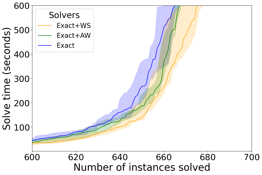
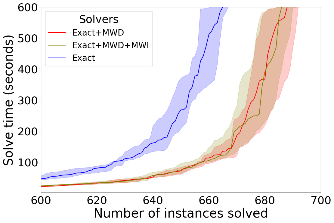
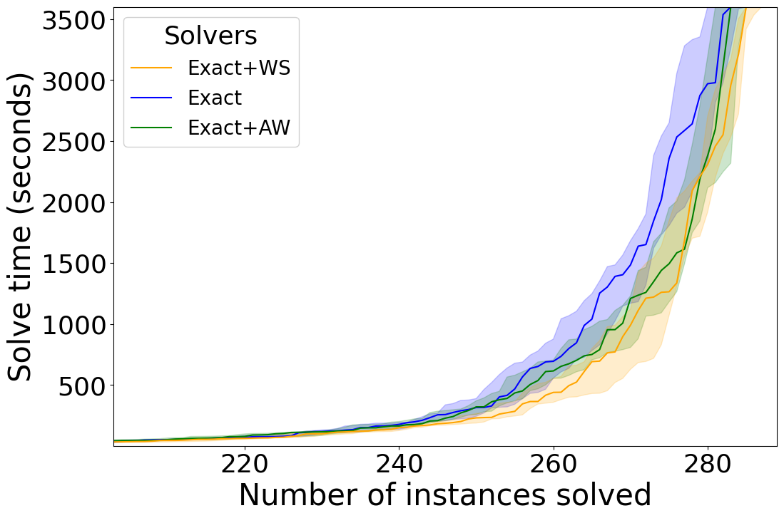
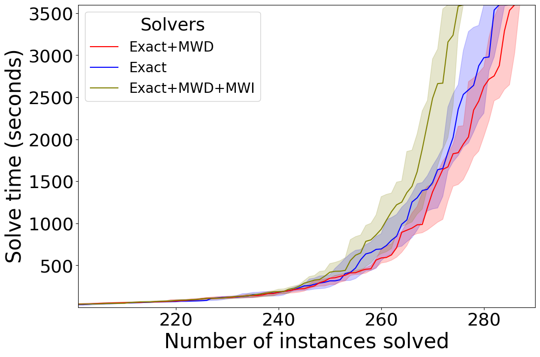
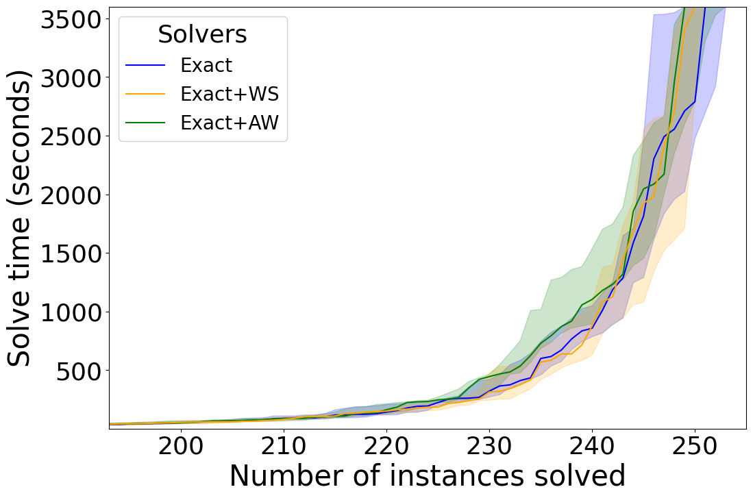
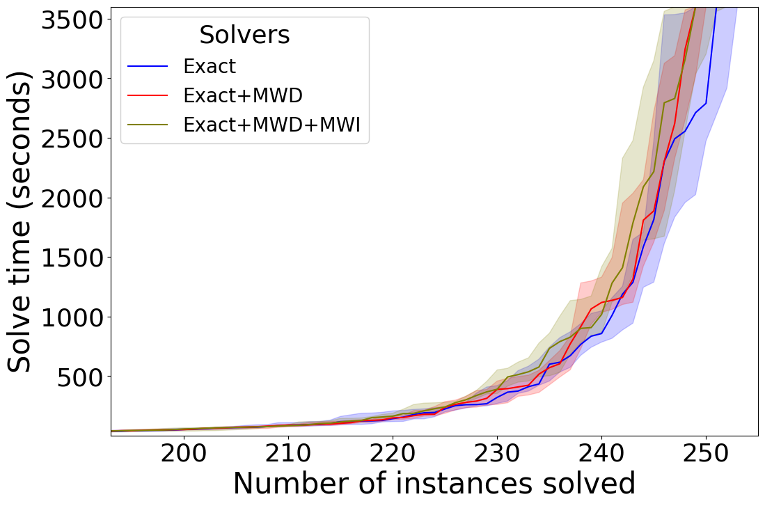
Our first experiment compares each individual technique (i.e. the WS, AW, MWD, and MWD+MWI reduction methods) to Exact as a baseline. For the division-based techniques we see that on KNAP in Figure 1(a), WS solves more instances and AW solves some instances faster. We also see positive results when it comes to the saturation-based techniques in Figure 1(b). MWD and MWD+MWI both perform similarly, while outperforming the baseline. On DEC-LIN we see similar trends for the division-based techniques in Figure 2(a). WS still solves more instances than the baseline and AW mostly helps solving some instances faster. For the saturation-based techniques we do see in Figure 2(b) a different trend compared to KNAP. While MWD still helps improve the performance of the solver, MWD+MWI shows a negative performance. This unexpected result is interesting, since we know MWD+MWI dominates MWD from a theoretical perspective. On OPT-LIN we do not see much of a difference either way for the division-based techniques in Figure 3(a), but the performance marginally worsens for the saturation-based techniques in Figure 3(b).

We believe the smaller impact of AW is due to how each technique changes the constraint. WS only lowers one coefficient while keeping everything else the same, while AW increases the degree as well as a coefficient. The increase in the degree could however lead to fewer saturation opportunities after addition with the conflict constraint, reducing the impact. On the other hand, lowering a coefficient via WS may lead to fewer variable cancellations and in turn less saturation after addition, though the odds for cancellation on non-propagated literals may be relatively smaller. In the end, both techniques show only moderate impact on the selected benchmarks.

In our second experiment we evaluate how combining the different techniques as shown in Section 4.3 impacts the empirical runtime of PB solvers. Additionally, we test an implementation of the combined division-based techniques, WS+AW, on another solver, namely the PB’24 competition version of RoundingSat, to see how it behaves in different solvers. Implementing the saturation-based techniques in RoundingSat would have required more extensive changes due to overflows after multiplication.

The results are summarised in Table 1. On KNAP, combining all the techniques has a compounding effect for both solvers. On DEC-LIN, the results are less clear. Exact+WS+AW does perform very well, which might initially seem surprising since according to Proposition 11 applying AW means less WS is possible. RoundingSat+WS+AW, on the other hand has minor impact on RoundingSat for DEC-LIN. Still, it seems both techniques can be combined effectively. The same cannot be said when mixing the division- and saturation-based techniques. We hypothesize that since WS+AW improves division-based reduction, a better heuristic than Equation 14 for the saturation-based techniques is necessary. It may be that WS+AW is most effective in many cases where MWD is actually possible, thus the improvements from WS+AW carry over to WS+AW+MWD. On OPT-LIN, the choice of configuration of the techniques still does not seem to have much impact, with similar performance to the configurations using an individual technique.

References

- [1] Gilles Audemard and Laurent Simon. On the glucose SAT solver. Int. J. Artif. Intell. Tools, 27(1):1840001:1–1840001:25, February 2018. doi:10.1142/S0218213018400018.
- [2] Danel Le Berre, Pierre Marquis, Stefan Mengel, and Romain Wallon. On Irrelevant Literals in Pseudo-Boolean Constraint Learning. In Proceedings of the Twenty-Ninth International Joint Conference on Artificial Intelligence, pages 1148–1154, July 2020. doi:10.24963/ijcai.2020/160.
- [3] Daniel Le Berre and Anne Parrain. The sat4j library, release 2.2. J. Satisf. Boolean Model. Comput., 7(2-3):59–6, 2010. doi:10.3233/sat190075.
- [4] Sam Buss and Jakob Nordström. Proof complexity and SAT solving. In Armin Biere, Marijn Heule, Hans van Maaren, and Toby Walsh, editors, Handbook of Satisfiability - Second Edition, volume 336 of Frontiers in Artificial Intelligence and Applications, pages 233–350. IOS Press, 2021. doi:10.3233/FAIA200990.
- [5] Donald Chai and Andreas Kuehlmann. A fast pseudo-boolean constraint solver. In Proceedings of the 40th Annual Design Automation Conference, pages 830–835, Anaheim CA USA, June 2003. ACM. doi:10.1145/775832.776041.
- [6] Donald Chai and Andreas Kuehlmann. A fast pseudo-boolean constraint solver. IEEE Transactions on Computer-Aided Design of Integrated Circuits and Systems, 24:305–317, 2005. doi:10.1109/TCAD.2004.842808.
- [7] Stephen A. Cook. The complexity of theorem-proving procedures. In Michael A. Harrison, Ranan B. Banerji, and Jeffrey D. Ullman, editors, Proceedings of the 3rd Annual ACM Symposium on Theory of Computing, May 3-5, 1971, Shaker Heights, Ohio, USA, STOC ’71, pages 151–158, New York, NY, USA, 1971. ACM. doi:10.1145/800157.805047.
- [8] W. Cook, C.R. Coullard, and Gy. Turán. On the complexity of cutting-plane proofs. Discrete Applied Mathematics, 18(1):25–38, September 1987. doi:10.1016/0166-218X(87)90039-4.
- [9] Jo Devriendt. Pisinger’s knapsack instances in opb format, July 2020. doi:10.5281/zenodo.3939055.
- [10] Jo Devriendt. Watched Propagation of 0-1 Integer Linear Constraints. In Helmut Simonis, editor, Principles and Practice of Constraint Programming, pages 160–176, Cham, 2020. Springer International Publishing. doi:10.1007/978-3-030-58475-7_10.
- [11] Jo Devriendt. Exact: Evaluating cutting-planes learning at the PB’24 competition. Slides, 2024.
- [12] Jan Elffers and Jakob Nordström. Divide and Conquer: Towards Faster Pseudo-Boolean Solving. In Proceedings of the Twenty-Seventh International Joint Conference on Artificial Intelligence, pages 1291–1299, Stockholm, Sweden, July 2018. International Joint Conferences on Artificial Intelligence Organization. doi:10.24963/ijcai.2018/180.
- [13] Jan Elffers and Jakob Nordström. RoundingSat 2019: Recent work on PB solving. https://slides.com/jod/deck-26-29-32, July 2019.
- [14] Armin Haken. The intractability of resolution. Theor. Comput. Sci., 39:297–308, 1985. Third Conference on Foundations of Software Technology and Theoretical Computer Science. doi:10.1016/0304-3975(85)90144-6.
- [15] John N Hooker. Generalized resolution and cutting planes. Annals of Operations Research, 12:217–239, 1988.
- [16] Hannes Ihalainen, Jeremias Berg, and Matti Järvisalo. Ipbhs in pb’24 competition. Slides, 2024.
- [17] Christoph Jabs, Jeremias Berg, and Matti Järvisalo. PB-OLL-RS and MIXED-BAG in Pseudo-Boolean Competition 2024. PB Competition 2024, 2024.
- [18] Daniel Le Berre, Pierre Marquis, and Romain Wallon. On Weakening Strategies for PB Solvers. In Luca Pulina and Martina Seidl, editors, Theory and Applications of Satisfiability Testing – SAT 2020, pages 322–331, Cham, 2020. Springer International Publishing. doi:10.1007/978-3-030-51825-7_23.
- [19] Orestis Lomis, Jo Devriendt, Hendrik Bierlee, and Tias Guns. ML-KULeuven/SAT25_PB_reductions_experiments. Dataset, This research was partly funded by the European Research Council (ERC) under the EU Horizon 2020 research and innovation programme (Grant No 101002802, CHAT-Opt)., swhId: swh:1:dir:650c2f9b37926504a59a11a6dbf319620b311dc3 (visited on 2025-07-23). URL: https://github.com/ML-KULeuven/SAT25_PB_reductions_experiments, doi:10.4230/artifacts.24089.
- [20] J.P. Marques Silva and K.A. Sakallah. Grasp-a new search algorithm for satisfiability. In Proceedings of International Conference on Computer Aided Design, pages 220–227, 1996. doi:10.1109/ICCAD.1996.569607.
- [21] Gioni Mexi, Timo Berthold, Ambros Gleixner, and Jakob Nordström. Improving conflict analysis in mip solvers by pseudo-boolean reasoning. arXiv preprint arXiv:2307.14166, 2023. doi:10.48550/arXiv.2307.14166.
- [22] Shiwei Pan, Yiyuan Wang, Shaowei Cai, Jiangnan Li, Wenbo Zhu, and Minghao Yin. Cashwmaxsat-disjcad: Solver description. MaxSAT Evaluation 2024, 2024:25, 2024.
- [23] David Pisinger. Where are the hard knapsack problems? Comput. Oper. Res., 32(9):2271–2284, 2005. doi:10.1016/j.cor.2004.03.002.
- [24] Roussel, Olivier. Pseudo-Boolean Competition of 2024. https://www.cril.univ-artois.fr/PB24/.