Symbolic Conflict Analysis in Pseudo-Boolean Optimization

In this paper, we go one step further and show how constraints learned when looking for a solution larger than $C$ can not only be reused, but also automatically strengthened so that a stronger version of them is available during the search for solutions larger than $C^{\prime }>C$. This is accomplished by considering $C$ as a symbolic variable and adapting conflict analysis to take care of this feature. As a by-product of this symbolic way of treating constraints, one can automatically extract upper bounds from them, thus giving an estimation of how far the solver is from reaching an optimal solution. Experimental results show that the overhead of this symbolic procedure is negligible, and that its ability to further prune the search space results in important runtime improvements.

Pseudo-Boolean optimization is a well-studied problem for which three main methods exist: Linear Search, Core-guided Search [13, 24, 9], and Implicit Hitting Set approaches [33, 32]. They are considered to be complementary in the type of instances for which they work best and solvers might even use combinations of them (e.g. RoundingSat combines Linear with Core-guided Search). Linear Search, which is the topic of this paper, has also been applied to the MaxSAT problem. Two prominent contributions in this direction are Pacose [27] and MaxCDCL solver [21, 22], which combines a branch and bound search with a lower-bounding procedure to prune the search space. As far as we know, no previous work uses a symbolic treatment of the objective function and no other linear-search method can compute upper bounds with no additional cost. Hence, we believe the community will benefit from the introduction of this novel technique and will develop additional ways to further exploit it.

This paper is organized as follows. After some preliminaries in Section 2, we revisit the conflict analysis procedure of PB solvers in Section 3. Section 4 presents the main contributions of this paper: the symbolic conflict analysis procedure and its additional ability to compute upper bounds. Experimental evidence of their positive impact on a solver and a careful analysis of the data collected is reported in Section 5. We conclude in Section 6, where we also outline future research directions.

Let $𝒳$ be a set of propositional variables. A literal is either a variable ($x$) or the negation of one ($\overline{x}$). We will assume that $\overline{\overline{x}}=x$. A (pseudo-Boolean or PB) constraint is a 0-1 linear inequality ${\sum }_i{c}_i{l}_i\ge d$ where the $l_i$’s are literals and, without loss of generality, the $c_i$’s (coefficients) and $d$ (degree) are positive integers. When all coefficients are $1$ we say that the constraint is a cardinality constraint and if, in addition, $d$ is also 1 we say that it is a $\mathrm{𝑐𝑙𝑎𝑢𝑠𝑒}$. A formula is a set of constraints.

An assignment $\rho$ is a set of non-contradictory literals. It is total if for any $x\in 𝒳$ either $x\in \rho$ or $\overline{x}\in \rho$, and partial otherwise. A literal $l$ is true in $\rho$ if $l\in \rho$, is false if $\overline{l}\in \rho$ and is undefined otherwise. Given a constraint $C$ of the form ${\sum }_i{c}_i{l}_i\ge d$, an assignment $\rho$ satisfies it if ${\sum }_{i:l_i\in \rho }{c}_i\ge d$, and falsifies it if no extension of $\rho$ can satisfy it. If we define $slack(C,\rho )=({\sum }_{i:\overline{l_i}\notin \rho }{c}_i)-d$, it can be seen that $\rho$ falsifies $C$ if and only if . Note the slack expression sums the coefficients of all non-false literals, and that is the maximum value that the left hand side of the constraint can reach. If even that does not exceed $d$, no extension of $\rho$ will do. An assignment that satisfies all constraints of a formula is called a model. A formula $F$ is a logical consequence of $G$ if any model of $G$ is also a model of $F$.

In order to determine the satisfiability of a set of constraints, one can use the cutting planes proof system, which consists of axioms $l\ge 0$ for all literals $l$, and the following two inference rules:

Linear combination:   $\begin{array}{cc}{\sum }_i{a}_i{l}_i\ge A\hspace{1em}{\sum }_i{b}_i{l}_i\ge B& \alpha ,\beta \in {\mathbb{N}}^{+}\\ \stackrel{\mathit{‾}}{{\sum }_i(\alpha a_i+\beta b_i)l_i\ge \alpha A+\beta B}\end{array}$

Division:         $\begin{array}{cc}{\sum }_i{a}_i{l}_i\ge A& \alpha \in {\mathbb{N}}^{+}\\ \stackrel{\mathit{‾}}{{\sum }_i\lceil a_i/\alpha \rceil l_i\ge \lceil A/\alpha \rceil }\end{array}$

It is well known [19] that a set of constraints is unsatisfiable if and only if $0\ge 1$ can be derived using these rules. We note that in the application of linear combination we implicitly assume that any constraint is simplified by using that fact that $l+\overline{l}=1$. For example, the constraint $2x+3\overline{x}+5y\ge 7$ can be rewritten as $2(x+\overline{x})+\overline{x}+5y\ge 7$ and is hence equivalent to $\overline{x}+5y\ge 5$. Another well-known rule, which is very useful in PB solving, limits coefficients to be at most equal to the degree:

Saturation:        $\begin{array}{c}{\sum }_i{a}_i{l}_i\ge A\\ \stackrel{\mathit{‾}}{{\sum }_{i}min(a_i,A)l_i\ge A}\end{array}$

Given a constraint $C={\sum }_i{c}_i{l}_i\ge d$ and an assignment $\rho$, we say that $C$ unit propagates $l_i$ under $\rho$ if $l_i$ is undefined in $\rho$, but $l_i$ is true in any total assignment extending $\rho$ that satisfies $C$. The latter is equivalent to checking whether , i.e., if we do not set $l_i$ to true, the constraint becomes falsified. Given a formula $F$ and an assignment $\rho$, unit propagation of $F$ under $\rho$ is the outcome of applying the following two rules until a fixpoint is reached: (i) if $\rho$ falsifies a constraint $C\in F$, a conflict is found with conflicting constraint $C$ and we stop, (ii) if $\rho$ unit propagates some literal $l$ due to constraint $C$, extend $\rho :=\rho \cup \{l\}$ with reason $C$.

A generalization of the well-known CDCL [23] algorithm for SAT can be applied to the pseudo-Boolean case [31]. The algorithm starts with an empty assignment $\rho$ and proceeds as follows: (1) Apply unit propagation, possibly extending $\rho$. (2) If a conflict is found, a conflict analysis procedure uses the aforementioned inference rules to derive a constraint $C$ (called lemma) that can be safely added to the formula. If $C$ is the constraint $0\ge 1$, the formula is unsatisfiable, otherwise it is guaranteed that after removing some literals from $\rho$ in a last-in first-out way (backjumping), $C$ allows some literal to be unit propagated. Hence, we go to step 1. (3) If no conflict is found, and $\rho$ is total, it is a model of the formula. Otherwise, an undefined literal $l$ (decision literal) is added to $\rho$ and we go to step 1. If we see $\rho$ as a sequence, any literal appearing in the sequence between the $k$-th decision literal (included) and before the $(k+1)$-th one is said to belong to decision level $k$.

Given a set $S$ of PB-constraint and an objective function ${\sum }_i{c}_i{l}_i$, the Pseudo-Boolean Optimization problem consists of finding, among all assignments that satisfy $S$, one that maximizes the value of the objective function. A very simple approach for this problem is to first run a PB solver to determine the satisfiability of $S$. If a solution is found, for which the objective function has value $C$, a constraint ${\sum }_i{c}_i{l}_i\ge C+1$ is added to $S$ and the same solver is launched again. Eventually, the solver will report the unsatisfiability of the augmented set of constraints, and the last found solution is an optimal one. This is sometimes known as the Linear Search approach to PB optimization.

Given a constraint $X\ge d$, we denote by $SNF(X,\rho )$ the (S)um of the coefficients of all literals in $X$ that are (N)on-(F)alse in $\rho$. It holds that $SNF(X,\rho )=slack(X\ge d,\rho )+d$.

Let us assume that neither $𝒞$ nor $𝒟$ are false in $\rho$ and reach a contradiction. Since $ℛ$ is false in $\rho$, we have that . Since we know that $ℛ$ is of the form $bC+aD\ge b{k}_c+a{k}_d-ab$, with no contradictory literals between $C$ and $D$, we have that $slack(ℛ,\rho )=SNF(bC+aD,\rho )-b{k}_c-a{k}_d+ab=bSNF(C,\rho )+aSNF(D,\rho )-b{k}_c-a{k}_d+ab$. Note that the last equality holds because $C$ and $D$ have no contradictory literals, otherwise cancellation between those literals could make it invalid. All in all, we can conclude that .

Now, since $𝒞$ is not false, we have that $slack(𝒞,\rho )\ge 0$ and hence $SNF(al+C,\rho )-k_c\ge 0$ and also $aSNF(l,\rho )+SNF(C,\rho )-k_c\ge 0$ and $abSNF(l,\rho )+bSNF(C,\rho )-b{k}_c\ge 0$. Similarly $abSNF(\overline{l},\rho )+aSNF(D,\rho )-a{k}_d\ge 0$. If we add these last two inequalities, and considering that $SNF(l,\rho )+SNF(\overline{l},\rho )=1$ because $l$ is assigned in $\rho$, we have that $ab+bSNF(C,\rho )+aSNF(D,\rho )-b{k}_c-a{k}_d\ge 0$, which contradicts the last inequality of the previous paragraph. $◀$

Apply Lemma 2 with assignment $\rho \cup \{{\overline{l}}_p\}$ and use the fact that a constraint $𝒞$ is false in $\rho \cup \{{\overline{l}}_p\}$ if and only if $𝒞$ propagates a literal $l_p$ under $\rho$. $◀$

We conclude this section with an example showing the execution of a CDCL-based PB solver that uses a conflict analysis method based on Algorithm 1. This allow us to show how our procedure of Section 4 is able to improve it. For simplicity, we have chosen an example for which the application of $weakenConstraints$ is never necessary.

Since no constraint is propagating, the solver decides on a literal, say $a$, which propagates $\overline{x}$ and $\overline{y}$ due to $C_1$. Next decision is $b$, which propagates $\overline{z}$ and $\overline{u}$ due to $C_2$. Next decision is $c$, which propagates $\overline{v}$ and $\overline{w}$ due to $C_3$. All constraints are satisfied and we have found a solution for which the objective function has value $0$.

Since we have to look for a better solution, constraint $C_4:=x+2y+3z+4u+5v+6w\ge 1$ is added. The solver makes the same decisions and propagations as before, but the assignment $\rho =(a^d,{\overline{x}}_1,{\overline{y}}_1,b^d,{\overline{z}}_2,{\overline{u}}_2,c^d,{\overline{v}}_3,{\overline{w}}_3)$, where a superscript $d$ indicates a decision and a subscript $i$ represents that constraint $C_i$ is the reason for that propagation, now falsifies constraint $C_4$. Conflict analysis is started, popping literal $\overline{w}$ from $\rho$, making $slck$ be 5 and the loop in lines $4-6$ terminate. Since $C_3$ is the reason for $\overline{w}$, and $\alpha =6,\beta =1$, the linear combination is $1\cdot C_4+6\cdot C_3$, which is $C_5:=6\overline{c}+x+2y+3z+4u+\overline{v}\ge 2$. This constraint propagates $\overline{c}$ at decision level 2, and hence the solver backjumps to produce assignment $\rho =(a^d,{\overline{x}}_1,{\overline{y}}_1,b^d,{\overline{z}}_2,{\overline{u}}_2,{\overline{c}}_5)$. No other constraint propagates and the solver now decides on $v$, which propagates $\overline{w}$ due to $C_3$ and $\rho$ is a solution with value $5$.

Since a better solution is needed we replace $C_4$ by $x+2y+3z+4u+5v+6w\ge 6$. The solver restarts and makes the same decisions and propagations to produce $\rho =(a^d,{\overline{x}}_1,{\overline{y}}_1,b^d,{\overline{z}}_2,{\overline{u}}_2)$. However, now $C_4$ propagates $w$ and, after that, $C_3$ propagates $\overline{v}$ and $\overline{c}$, which produces a solution with value $6$.

$C_4$ now becomes $x+2y+3z+4u+5v+6w\ge 7$. The solver restarts and proceeds as before to reach $\rho =(a^d,{\overline{x}}_1,{\overline{y}}_1,b^d,{\overline{z}}_2,{\overline{u}}_2)$. Now $C_4$ propagates $v$ and $w$ and the resulting assignment $\rho =(a^d,{\overline{x}}_1,{\overline{y}}_1,b^d,{\overline{z}}_2,{\overline{u}}_2,v_4,w_4)$ falsifies constraint $C_3$ The loop at lines $4-6$ pops $w$ from $\rho$, making $slck$ to be $0$. Since the coefficient of $w$ in the reason of $w$ is $\beta =6$ and the coefficient of $\overline{w}$ in $C_3$ is $\alpha =1$ the linear combination computed is $6\cdot C_3+1\cdot C_4$, which is $C_{tmp}:=6\overline{c}+x+2y+3z+4u+\overline{v}\ge 8$. Since this constraint does not propagate at any previous decision level, one more iteration of conflict analysis is required. The loop at lines 4-6 pops literals $v$ and $\overline{u}$, after which the $slck$ is 3 and the loop terminates. The procedure will now try to eliminate $\overline{u}$ from $C_{tmp}$ by performing an appropriate linear combination with the reason for $\overline{u}$, which is $C_2$. This linear combination is $1\cdot C_{tmp}+4\cdot C_2$, which results in $C_6:=4\overline{b}+6\overline{c}+x+2y+\overline{z}+\overline{v}\ge 9$. This constraint is learned since it allows the solver to backjump to decision level 1 and propagate $\overline{c}$ and $\overline{b}$. The assignment is now $\rho =(a^d,{\overline{x}}_1,{\overline{y}}_1,{\overline{c}}_6,{\overline{b}}_6)$. No other constraint propagates and the solver decides on $v$, which propagates $\overline{w}$ due to $C_3$. Next decision is on $u$, which propagates $\overline{z}$ due to $C_2$. The current assignment $\rho$ is a solution with value $9$.

$C_4$ now becomes $x+2y+3z+4u+5v+6w\ge 10$. Let us now remark that the solver, apart from the original constraints, only has the lemmas:

The solver restarts and, since no constraint propagates at decision level zero, it will decide on $a$. However, as we will show in the next section, this can be done much better.

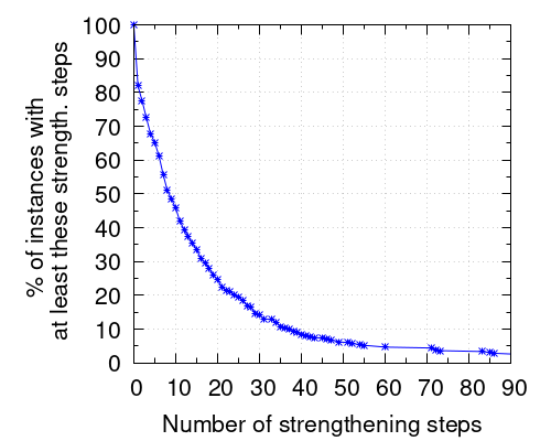
After every new solution is found, except for the first one, our symbolic conflict analysis procedure performs a strengthening step: it changes the degree of all symbolic constraints. Hence, having a systematic low number of strengthening steps on all benchmarks would indicate that our procedure is rarely applicable. In order to confirm that this pessimistic scenario is not common we computed, for all 385 benchmarks, how many such steps are done within one hour. This information is summarized in the leftmost cumulative plot of Figure 1.

A point $(x,y)$ in the plot means that there exist $y\%$ of the benchmarks for which at least $x$ strengthening steps are applied. For example, around 50% of the benchmarks have at least 8 steps, one third of them has at least 15 steps, and 20% of the benchmarks have at least 24 steps. Hence, the important message one has to infer from the plot is that it is very common that a non-negligible number of strengthening steps are used. There are some instances, left out of the plot for readability, with an unusually large number of steps: 4 benchmarks with between 100 and 150 steps, 2 benchmarks between 151 and 200, and 2 benchmarks with more than 201, being 255 the maximum one. There are also extreme cases on the opposite direction: for about 18% of the benchmarks no strengthening step was applied. This is not a huge number but we believe it is large enough so that it is not negligible: doing expensive computations to later realize that our technique is not applicable at all would definitely slow down the solver on around 20% of the instances.

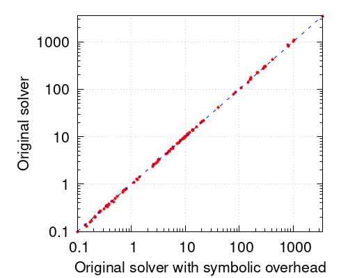
Fortunately, the rightmost scatter plot of Figure 1 reveals how surprisingly small the overhead of symbolic conflict analysis is. For precisely assessing this overhead, we implemented our symbolic procedure on top of our solver: all constraints have a symbolic part; linear combination, saturation and division are applied taking into account this symbolic part but, after a new solution is found, the strengthened degree of all symbolic constraints is computed but not updated. That is, we pay all the overhead of our procedure but, since the constraints are unchanged, the solver has the same search behavior as its baseline version. The scatter plot compares the runtime in seconds of this modified system and our original solver. It is entirely obvious that the overhead caused by the symbolic procedure is negligible. We want to remark that this is the case independently of the package we use for infinite-precision rational numbers on the symbolic part: we tried GMP [14], Boost [5] and a custom package developed in our research group and no differences were observed.

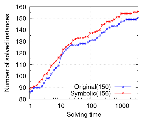
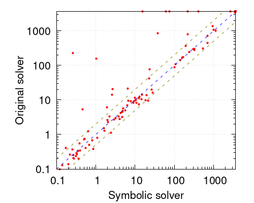
Let us now show that implementing symbolic conflict analysis on top of our solver produces important performance gains. The CDF plot on the left of Figure 2 shows how the addition of the symbolic conflict analysis procedure makes the solver able to solve more problems within any given time limit. For a time limit of 1 hour the solver is able to solve 6 more benchmarks up to optimality. The scatter plot on the right contains two parallel green lines delimiting speedups of 2x. We can see that despite there are concrete instances for which the symbolic solver is slower, they are mostly easy instances solved within 30 seconds, and the slowdown is never larger than 2x. On the other hand, there are several benchmarks for which the symbolic solver outperforms the baseline by very large speedup factors.

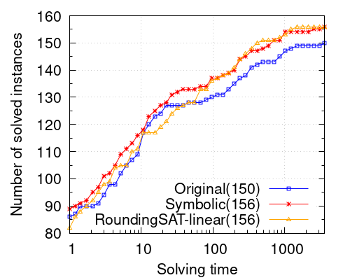
Finally, we want to compare our system with the state of the art. For this purpose we chose the latest version of RoundingSat [11, 9, 8]. Note that, in the optimization linear constraints category of the 2024 Pseudo-Boolean Competition, 8 of the 10 best performing solvers used RoundingSat, either as an oracle or combined with additional techniques. We ran RoundingSat in linear-search mode. Despite its full version, which combines linear and core-guided search is more powerful, the purpose of this comparison is limited to linear search. The CDF plot on Figure 3 shows how our original solver is slower than RoundingSat. This might be due to maturity of the implementation, different search strategies and, more importantly, concrete details in conflict analysis related to different weakening procedures, different uses of saturation and division, and termination criteria of the main loop as we explained in Section 3. However, the addition of symbolic conflict analysis bridges this gap and makes them behave more similarly. As we will mention, it is part of our future work to examine how symbolic conflict analysis can improve the linear-search component of other solvers, and RoundingSat is definitely a candidate.

In the optimization linear constraints category, 8 of the 10 best performing solvers did use RoundingSAT. That is, it was either used as an oracle or combined with additional techniques. Hence, it is at the core of almost every solver, except for SCIP.

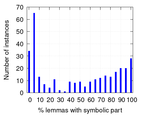
The next question we want to address is to determine how many lemmas have a non-constant symbolic part, that is, $⟦p\cdot \delta +q⟧$ with $p\ne 0$. The left histogram in Figure 4 summarizes this information. For each of the 312 out of the overall 385 benchmarks that apply some strengthening step, whenever this step is performed we compute the percentage of PB constraints that have a non-constant symbolic part. Note that in our solver clauses have a particular treatment and they are not considered as PB constraints in this computation. When the execution finishes, we compute the average over all strengthening steps of these percentages. The histogram essentially represents this average. More concretely, the first bar indicates that for 34 benchmarks this average is zero. The second bar shows that for 65 benchmarks this average is in the interval $(0,5]$; the third bar over the 10 label means that the average is in (5,10] for 13 benchmarks, and so on. As expected from the previous results on performance, the percentage of constraints with non-constant symbolic part is remarkable, making the strengthening step a powerful one.

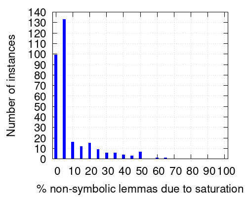
Another question we wanted to answer is to discover the reasons why certain lemmas are non-symbolic (i.e. $p=0$ in $⟦p\cdot \delta +q⟧$). One obvious reason is that it might happen that the constraint bounding the objective function has not been used in the derivation of this lemma. Another possibility is the interaction between saturation and our symbolic procedure, as we explained in Section 4.3. In our implementation, whenever saturation is to be applied on a constraint with non-constant symbolic part, we apply it and remove its symbolic information. If this happens too often, it could hinder the power of our symbolic reasoning. The right histogram in Figure 4 answers this question in a positive way: this situation is not common at all. For example, the bar with height 15 over the 20 label means that there are 15 instances for which, if we only consider non-symbolic constraints, the percentage of them that are non-symbolic due to an application of saturation is in the interval $(15,20]$. As we can see, the main reason for a constraint not being symbolic is not the application of saturation.

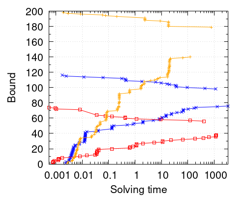
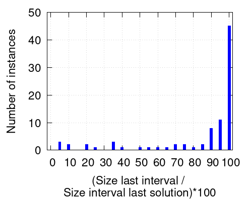
An interesting feature of our procedure is the computation of upper bounds. The number of times that our procedure improves the upper bound is significant for several benchmarks. In the left plot of Figure 5 we can see, for three concrete instances, the evolution of the upper and the lower bound. Since these instances are minimization problems, finding a new solution improves the upper bound, whereas our new bounding techniques improve the lower bound. We can see that both bounds are improved several times during the execution of the system. However, we want to note that there are of course instances for which the production of new bounds is not as frequent. This is observed in the right plot of Figure 5. We have considered all 87 benchmarks for which our solver timed out in one hour and such that after the last solution found, our bounding technique is able to reduce the size of the interval $[LB,UB]$. The plot displays the number of instances for which the size of the last interval produced by the solver, divided by the size of the interval after the last solution was found is equal to a certain number. A small number implies that our bounding technique is able to produce a significant reduction on the interval size since the last found solution. As we can see, although for half of the benchmarks only small reductions are achieved, for the other half it does have a beneficial effect, with different magnitudes depending on the benchmark. This shows that, even when the solver is not able to find further solutions, the bounding technique still makes progress in the estimation of the optimum.

It is well known that in PB optimization, binary search is generally outperformed by linear search. Unfortunately, according to our experiments, this is still the case even if one is able to reuse all lemmas from all problems, as we can do thanks to our symbolic procedure.

References

- [1] Elvira Albert, Pablo Gordillo, Alejandro Hernández-Cerezo, and Albert Rubio. A max-smt superoptimizer for EVM handling memory and storage. In Dana Fisman and Grigore Rosu, editors, Tools and Algorithms for the Construction and Analysis of Systems – 28th International Conference, TACAS 2022, Held as Part of the European Joint Conferences on Theory and Practice of Software, ETAPS 2022, Munich, Germany, April 2-7, 2022, Proceedings, Part I, volume 13243 of Lecture Notes in Computer Science, pages 201–219. Springer, 2022. doi:10.1007/978-3-030-99524-9_11.
- [2] Albert Atserias, Johannes Klaus Fichte, and Marc Thurley. Clause-learning algorithms with many restarts and bounded-width resolution. J. Artif. Intell. Res., 40:353–373, 2011. doi:10.1613/jair.3152.
- [3] Daniel Le Berre, Pierre Marquis, and Romain Wallon. On weakening strategies for PB solvers. In Luca Pulina and Martina Seidl, editors, Theory and Applications of Satisfiability Testing – SAT 2020 – 23rd International Conference, Alghero, Italy, July 3-10, 2020, Proceedings, volume 12178 of Lecture Notes in Computer Science, pages 322–331. Springer, 2020. doi:10.1007/978-3-030-51825-7_23.
- [4] Armin Biere and Daniel Kröning. Sat-based model checking. In Edmund M. Clarke, Thomas A. Henzinger, Helmut Veith, and Roderick Bloem, editors, Handbook of Model Checking, pages 277–303. Springer, 2018. doi:10.1007/978-3-319-10575-8_10.
- [5] The Boost C++ libraries. Available at https://www.boost.org/.
- [6] Donald Chai and Andreas Kuehlmann. A fast pseudo-boolean constraint solver. IEEE Trans. on CAD of Integrated Circuits and Systems, 24(3):305–317, 2005. doi:10.1109/TCAD.2004.842808.
- [7] W. Cook, C. Coullard, and Gy. Turan. On the complexity of cutting-plane proofs. Discrete Applied Mathematics, 18:25–38, 1987. doi:10.1016/0166-218X(87)90039-4.
- [8] Jo Devriendt, Ambros M. Gleixner, and Jakob Nordström. Learn to relax: Integrating 0-1 integer linear programming with pseudo-boolean conflict-driven search. Constraints An Int. J., 26(1):26–55, 2021. doi:10.1007/S10601-020-09318-X.
- [9] Jo Devriendt, Stephan Gocht, Emir Demirovic, Jakob Nordström, and Peter J. Stuckey. Cutting to the core of pseudo-boolean optimization: Combining core-guided search with cutting planes reasoning. In Thirty-Fifth AAAI Conference on Artificial Intelligence, AAAI 2021, Thirty-Third Conference on Innovative Applications of Artificial Intelligence, IAAI 2021, The Eleventh Symposium on Educational Advances in Artificial Intelligence, EAAI 2021, Virtual Event, February 2-9, 2021, pages 3750–3758. AAAI Press, 2021. doi:10.1609/AAAI.V35I5.16492.
- [10] Julian Dolby, Mandana Vaziri, and Frank Tip. Finding Bugs Efficiently With a SAT Solver. In Proceedings of the 6th joint meeting of the European Software Engineering Conference and the ACM SIGSOFT International Symposium on Foundations of Software Engineering, pages 195–204, 2007. doi:10.1145/1287624.1287653.
- [11] Jan Elffers and Jakob Nordström. Divide and conquer: Towards faster pseudo-boolean solving. In Jérôme Lang, editor, Proceedings of the Twenty-Seventh International Joint Conference on Artificial Intelligence, IJCAI 2018, July 13-19, 2018, Stockholm, Sweden, pages 1291–1299. ijcai.org, 2018. doi:10.24963/ijcai.2018/180.
- [12] Nick Feng and Fahiem Bacchus. Clause size reduction with all-uip learning. In Luca Pulina and Martina Seidl, editors, Theory and Applications of Satisfiability Testing – SAT 2020 – 23rd International Conference, Alghero, Italy, July 3-10, 2020, Proceedings, volume 12178 of Lecture Notes in Computer Science, pages 28–45. Springer, 2020. doi:10.1007/978-3-030-51825-7_3.
- [13] Zhaohui Fu and Sharad Malik. On solving the partial MAX-SAT problem. In Armin Biere and Carla P. Gomes, editors, Theory and Applications of Satisfiability Testing – SAT 2006, 9th International Conference, Seattle, WA, USA, August 12-15, 2006, Proceedings, volume 4121 of Lecture Notes in Computer Science, pages 252–265. Springer, 2006. doi:10.1007/11814948_25.
- [14] The GNU MP Bignum Library. Available at https://gmplib.org/.
- [15] Stephan Gocht, Jakob Nordström, and Amir Yehudayoff. On division versus saturation in pseudo-boolean solving. In Sarit Kraus, editor, Proceedings of the Twenty-Eighth International Joint Conference on Artificial Intelligence, IJCAI 2019, Macao, China, August 10-16, 2019, pages 1711–1718. ijcai.org, 2019. doi:10.24963/IJCAI.2019/237.
- [16] Ana Graça, João Marques-Silva, Inês Lynce, and Arlindo L. Oliveira. Efficient haplotype inference with combined CP and OR techniques. In Laurent Perron and Michael A. Trick, editors, Integration of AI and OR Techniques in Constraint Programming for Combinatorial Optimization Problems, 5th International Conference, CPAIOR 2008, Paris, France, May 20-23, 2008, Proceedings, volume 5015 of Lecture Notes in Computer Science, pages 308–312. Springer, 2008. doi:10.1007/978-3-540-68155-7_28.
- [17] Armin Haken. The intractability of resolution. Theoretical Computer Science, 39(2 & 3):297–308, 1985. doi:10.1016/0304-3975(85)90144-6.
- [18] Marijn J. H. Heule, Oliver Kullmann, and Victor W. Marek. Solving and verifying the boolean pythagorean triples problem via cube-and-conquer. In Nadia Creignou and Daniel Le Berre, editors, Theory and Applications of Satisfiability Testing – SAT 2016 – 19th International Conference, Bordeaux, France, July 5-8, 2016, Proceedings, volume 9710 of Lecture Notes in Computer Science, pages 228–245. Springer, 2016. doi:10.1007/978-3-319-40970-2_15.
- [19] John N Hooker. Generalized resolution and cutting planes. Annals of Operations Research, 12:217–239, 1988.
- [20] Dejan Jovanovic and Leonardo Mendonça de Moura. Cutting to the chase – solving linear integer arithmetic. J. Autom. Reasoning, 51(1):79–108, 2013. doi:10.1007/s10817-013-9281-x.
- [21] Chu-Min Li, Zhenxing Xu, Jordi Coll, Felip Manyà, Djamal Habet, and Kun He. Combining clause learning and branch and bound for maxsat. In Laurent D. Michel, editor, 27th International Conference on Principles and Practice of Constraint Programming, CP 2021, Montpellier, France (Virtual Conference), October 25-29, 2021, volume 210 of LIPIcs, pages 38:1–38:18. Schloss Dagstuhl – Leibniz-Zentrum für Informatik, 2021. doi:10.4230/LIPICS.CP.2021.38.
- [22] Chu-Min Li, Zhenxing Xu, Jordi Coll, Felip Manyà, Djamal Habet, and Kun He. Boosting branch-and-bound maxsat solvers with clause learning. AI Commun., 35(2):131–151, 2022. doi:10.3233/AIC-210178.
- [23] João Marques-Silva, Inês Lynce, and Sharad Malik. Conflict-driven clause learning SAT solvers. In Armin Biere, Marijn Heule, Hans van Maaren, and Toby Walsh, editors, Handbook of Satisfiability – Second Edition, volume 336 of Frontiers in Artificial Intelligence and Applications, pages 133–182. IOS Press, 2021. doi:10.3233/FAIA200987.
- [24] António Morgado, Federico Heras, Mark H. Liffiton, Jordi Planes, and João Marques-Silva. Iterative and core-guided maxsat solving: A survey and assessment. Constraints An Int. J., 18(4):478–534, 2013. doi:10.1007/S10601-013-9146-2.
- [25] Robert Nieuwenhuis and Albert Oliveras. On SAT Modulo Theories and Optimization Problems. In Proceedings of SAT ’06, volume 4121 of Lecture Notes in Computer Science, pages 156–169. Springer, 2006. doi:10.1007/11814948_18.
- [26] Robert Nieuwenhuis, Albert Oliveras, Enric Rodríguez-Carbonell, and Emma Rollon. Employee scheduling with sat-based pseudo-boolean constraint solving. IEEE Access, 9:142095–142104, 2021. doi:10.1109/ACCESS.2021.3120597.
- [27] Tobias Paxian and Bend Becker. Pacose: An Iterative SAT-based MaxSAT Solver. In Jeremias Berg, Matti Järvisalo, Ruben Martins, Andreas Niskanen, and Tobias Paxian, editors, MaxSAT Evaluation 2024 : Solver and Benchmark Descriptions, Department of Computer Science Series of Publications B, page 26. University of Helsinki, 2024. URL: http://hdl.handle.net/10138/584878.
- [28] Knot Pipatsrisawat and Adnan Darwiche. On the power of clause-learning SAT solvers as resolution engines. Artif. Intell., 175(2):512–525, 2011. doi:10.1016/j.artint.2010.10.002.
- [29] Albert Oliveras Robert Nieuwenhuis and Enric Rodríguez-Carbonell. Intsat: integer linear programming by conflict-driven constraint learning. Optimization Methods and Software, 2023. doi:10.1080/10556788.2023.2246167.
- [30] J.A. Robinson. A Machine-Oriented Logic Based on the Resolution Principle. Journal of the ACM, JACM, 12(1):23–41, 1965. doi:10.1145/321250.321253.
- [31] Olivier Roussel and Vasco M. Manquinho. Pseudo-boolean and cardinality constraints. In A. Biere, M. Heule, H. van Maaren, and T. Walsh, editors, Handbook of Satisfiability, volume 185 of Frontiers in AI and Applications, pages 695–733. IOS Press, 2009. doi:10.3233/978-1-58603-929-5-695.
- [32] Pavel Smirnov, Jeremias Berg, and Matti Järvisalo. Pseudo-boolean optimization by implicit hitting sets. In Laurent D. Michel, editor, 27th International Conference on Principles and Practice of Constraint Programming, CP 2021, Montpellier, France (Virtual Conference), October 25-29, 2021, volume 210 of LIPIcs, pages 51:1–51:20. Schloss Dagstuhl – Leibniz-Zentrum für Informatik, 2021. doi:10.4230/LIPICS.CP.2021.51.
- [33] Pavel Smirnov, Jeremias Berg, and Matti Järvisalo. Improvements to the implicit hitting set approach to pseudo-boolean optimization. In Kuldeep S. Meel and Ofer Strichman, editors, 25th International Conference on Theory and Applications of Satisfiability Testing, SAT 2022, August 2-5, 2022, Haifa, Israel, volume 236 of LIPIcs, pages 13:1–13:18. Schloss Dagstuhl – Leibniz-Zentrum für Informatik, 2022. doi:10.4230/LIPICS.SAT.2022.13.
- [34] Mate Soos, Karsten Nohl, and Claude Castelluccia. Extending SAT solvers to cryptographic problems. In Oliver Kullmann, editor, Theory and Applications of Satisfiability Testing – SAT 2009, 12th International Conference, SAT 2009, Swansea, UK, June 30 – July 3, 2009. Proceedings, volume 5584 of Lecture Notes in Computer Science, pages 244–257. Springer, 2009. doi:10.1007/978-3-642-02777-2_24.
- [35] Yichen Xie and Alexander Aiken. Saturn: A SAT-Based Tool for Bug Detection. In Proceedings of the 17th International Conference on Computer Aided Verification, CAV 2005, pages 139–143, 2005. doi:10.1007/11513988_13.
- [36] L. Zhang, C. F. Madigan, M. W. Moskewicz, and S. Malik. Efficient Conflict Driven Learning in a Boolean Satisfiability Solver. In International Conference on Computer-Aided Design, ICCAD ’01, pages 279–285, 2001.