Spark: Sparsified Hierarchical Energy Minimization of RNA Pseudoknots

Gray, Mateo; Will, Sebastian; Jabbari, Hosna

doi:10.4230/LIPIcs.WABI.2025.13

Spark: Sparsified Hierarchical Energy Minimization of RNA Pseudoknots

Mateo Gray

Department of Biomedical Engineering, University of Alberta, Edmonton, Canada Sebastian Will

Department of Computer Science, Institut Polytechnique de Paris, France Hosna Jabbari¹¹1Corresponding author

Department of Biomedical Engineering, University of Alberta, Edmonton, Canada

Abstract

Motivation.

Determining RNA structure is essential for understanding RNA function and interaction networks. Although experimental techniques yield high-accuracy structures, they are costly and time-consuming; thus, computational approaches – especially minimum-free-energy (MFE) prediction algorithms – are indispensable. Accurately predicting pseudoknots, however, remains challenging because their inclusion usually leads to prohibitive computational complexity. Recent work demonstrated that sparsification can improve the efficiency of complex pseudoknot prediction algorithms such as Knotty. This finding suggests similar gains are possible for already efficient algorithms like HFold, which targets a complementary class of hierarchically constrained pseudoknots.

Results.

We introduce Spark, an exact, fully sparsified algorithm for predicting pseudoknotted RNA structures. Like its non-sparsified predecessor HFold, Spark searches for the minimum-energy structure under the HotKots 2.0 energy model, a pseudoknot extension of the Turner model. Because the sparsification is non-heuristic, Spark preserves the asymptotic time- and space-complexity guarantees of HFold while greatly reducing the constant factors. We benchmarked the performance of Spark against HFold and, as a pseudoknot-free baseline, RNAfold. Compared with HFold, Spark substantially lowers both run time and memory usage, while achieving run-time figures close to those of RNAfold. Across all tested sequence lengths, Spark used the least memory and consistently ran faster than HFold.

Conclusion.

By extending non-heuristic sparsification to hierarchical pseudoknot prediction, Spark delivers an exceptionally fast and memory-efficient tool accurate prediction of pseudoknotted RNA structures, enabling routine analysis of long sequences. The algorithm broadens the practical scope of computational RNA biology and provides a solid foundation for future advances in structure-based functional annotation.

Availability.

Spark’s implementation and detailed results are available at https://github.com/TheCOBRALab/Spark.

Keywords and phrases:

RNA, MFE, Secondary Structure Prediction, Pseudoknot, Sparsification, Space Complexity, Time Complexity

Copyright and License:

2012 ACM Subject Classification:

Applied computing

\rightarrow

Computational biology

Supplementary Material:

Software (Source Code): https://github.com/TheCOBRALab/Spark [8]
archived at

swh:1:dir:2cb07371af448bb6254c05d23ac106800c590d39

DOI:

10.4230/LIPIcs.WABI.2025.13

Event:

25th International Conference on Algorithms for Bioinformatics (WABI 2025)

Editors:

Broňa Brejová and Rob Patro

Series and Publisher:

Leibniz International Proceedings in Informatics, Schloss Dagstuhl – Leibniz-Zentrum für Informatik

1 Introduction

RNA molecules carry out essential biological functions that often depend critically on their specific structural conformations [4, 15, 17, 21, 24]. Accordingly, a thorough understanding of many biological systems demands accurate models of RNA structure. Because experimental determination of RNA conformations is both costly and time-consuming, computational methods have become indispensable. These approaches not only complement experimental techniques by generating rapid structural hypotheses, but also enable new lines of inquiry, such as probing thermodynamic ensembles, exploring folding kinetics, and pursuing the rational design of functional RNAs.

A promising class of computational methods focuses on RNA secondary structure, where structure prediction can be formalized as combinatorial optimization problem of finding minimum-free-energy (MFE) structures. These techniques profit from energy models with accurate empirically determined energy parameters [16], known as nearest neighbor models or specifically, the “Turner model”, and efficient dynamic programming optimization algorithms. Consequently, they can predict realistic RNA secondary structures with high accuracy.

However, most practically applied algorithms in this class are restricted to pseudoknot-free structures, even though pseudoknots are common in RNAs; this limitation reduces their accuracy and constrains their application range.

Exact and accurate pseudoknot prediction.

To predict pseudoknotted RNA secondary structures with high accuracy, several advanced dynamic-programming algorithms have been developed [20, 14]. These methods extend the well-established Turner nearest-neighbor framework by incorporating empirically trained pseudoknot parameters, such as those in the HotKnots 2.0 energy model [5, 18]. Nevertheless, they are often limited by extreme computational complexity, e.g. $O(n^{6})$ time and $O(n^{4})$ space in the sequence length $n$ [20], and sometimes still support only simple pseudoknots, e.g. [5] in $O(n^{5})$ time.

While heuristics (e.g. [18]) were presented to overcome the computational limitations, we advocate the use of exact combinatorial methods that yield exact, controlled and precisely defined solutions. By restricting attention to well-chosen classes of pseudoknots and applying targeted algorithmic optimizations – most notably sparsification – one can achieve both tractability and broad practical utility.

We demonstrated this principle previously with the Chen,Condon,Jabbari (CCJ) algorithm and its fully featured successor, Knotty. Space-efficient sparsification of the CCJ recurrences enabled Knotty to compute MFE structures containing complex motifs such as 4-chains pseudoknots and kissing hairpins [14].

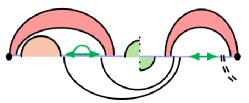
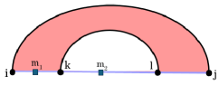
For even greater efficiency, we previously introduced hierarchical pseudoknot prediction in HFold [11, 12]. Fast enough to serve as the backbone of meta-strategies [10] and to fold long RNA sequences, HFold predicts a wide, biologically relevant class of pseudoknots. It complements an input non-crossing structure with a second, independently non-crossing structure that may cross the first, thereby generating density-2 configurations (see Fig. 1 and [13, 14]).

Figure 1: Band configuration of a density-2 structure. Bands and density-2 are elaborated in [13, 14]; here, we recall their definitions. The pseudoknotted base pairs of a structure can be partitioned into bands; all base pairs within one band are mutually nested and cross the exact same other base pairs of the structure. A set of bands can be further decomposed into components of transitively crossing bands, here {a,b,c,d} and {f,g}. The density-

k

property requires that no position is covered by more than

k

base pairs of the same component. For example, the position at the dashed red line satisfies density-2, since it is covered by the bands

d

,

f

and

g

, where only two of them are from the same component.

Contributions.

Further extending pseudoknot prediction capabilities, we introduce the sparsified dynamic programming algorithm Spark to predict hierarchically constrained pseudoknots. It solves exactly the same problem as HFold of predicting density-2 structures as extension of a given secondary structure. While Spark preserves the asymptotic complexity of HFold, it significantly improves practical run-time and space consumption due to sparsification.

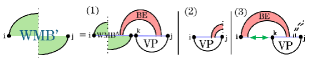
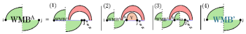
We outline the recurrences of the novel algorithm Spark, contrasting them to HFold and focusing on the requirements of sparsification. We show the correctness of the sparsification and illustrate the algorithm using graphical notation (see Fig. 2). Finally, we empirically show the improvements over HFold and compare to RNAfold for reference.

Further remarks on sparsification.

Sparsification was originally suggested to non-heuristically improve the time [22] and even the space efficiency [3] of pseudoknot-free RNA secondary structure prediction. It has been applied to more complex prediction tasks, e.g. interaction prediction [7]. These techniques can reduce time and space of prediction even in accurate RNA energy models [23] and accounting for dangling ends (SparseRNAFolD [9]). In the latter work, we closed a significant gap in utilizing of sparsification with realistic energy models, by demonstrating sparsified MFE folding with dangling ends for the pseudoknot-free case. This allowed us to surpass RNAfold [6] for the equivalent task.

As the key idea, sparsification limits the minimization cases in the dynamic programming (DP) recursions to only candidate subproblems. This is done, by omitting non-candidate cases, that provably are not required to compute the exact minima. In predicting the (non-crossing) MFE structure given a sequence $S$ , sparsification exploits the subadditivity of the MFE of subsequences from $i$ to $j$ . Namely, denoting the MFE by $W_{i,j}$ , the additive energy model implies the inverse triangle inequality $W_{i,j}\leq W_{i,k}+W_{k+1,j}$ $(i<k<j-1)$ [22].

For pseudoknot-free MFE, sparsification can thus reduce the time complexity from $O(n^{3})$ to $O(n^{2}+nZ)$ in the number of candidates $Z$ [22]. It was demonstrated that minimizing energy only requires to store the candidates and a linear number of subproblems. In nearest neighbor energy models, the optimal structure can be reconstructed by recording a set of trace arrows [23], of typically small size $T$ . This leads to a space complexity of $O(n+Z+T)$ . Our novel algorithm Spark achieves the same time complexity and similar space complexity for pseudoknot MFE prediction.

2 Review of hierarchical pseudoknot prediction in HFold

The recurrences of HFold for (non-sparsified) hierarchical pseudoknot prediction were introduced in [11, 12]. We begin with a concise overview of HFold ’s dynamic-programming algorithm, since Spark follows the same overall framework.

HFold’s input consists of an RNA sequence $S$ as well as a pseudoknot-free secondary structure $G$ . In the hierarchical folding scheme, the supplied input structure forms the primary, first-folding layer of the complete structure. HFold then computes a second disjoint pseudoknot-free structure $G^{\prime}$ such that the energy of the combined structure $G\cup G^{\prime}$ is minimized. As noted in the Introduction, HFold is designed to produce density-2 structures (Fig. 1). More precisely, each output can be viewed as a density-2 extension of the given input structure. We illustrate the recurrences of HFold and Spark using systematic graphical notation, which is shown for reference in Figure 2.

Refer to caption — Figure 2: Reference of graphical notation. This notation is used consistently in all of our illustrations of the recurrences of Spark and HFold. Dashed arcs indicate possible structure, each solid arc represents a base pair. The vertical dotted line indicates an overlapping chain of bands of arbitrary length and indicates that the chain can begin or end via $G$ (above horizontal line) or $G^{\prime}$ (below horizontal line). Filled in arcs show regions covered by specific structure classes, e.g. orange for $V$ , and green for $W\!M\!B$ . Green bidirectional arrows represent a nested structure inside a pseudoknot ( $W\!I$ ), while arrows that include an arc represent a nested structure inside a band ( $W\!I^{\prime}$ ).

Let us define an RNA sequence of size $n$ as $S=s_{1}s_{2}...s_{n}$ , where $s_{k}$ , $1\leq k\leq n$ is a nucleotide in $\{A,C,G,U\}$ . $W_{i,j}$ denotes the MFE of a substructure of the subsequence $S_{i..j}=s_{i}s_{i+1}...s_{j}$ .

In a density-2 structure, the terminal positions $i$ and $j$ of any substructure can close a loop in exactly two ways. (1) The nucleotides at positions $i$ and $j$ form a single base pair $(i,j)$ , thereby completing an ordinary, non-crossing loop. (2) The endpoints are connected by a chain of crossing base pairs $i_{1}.j_{1},i_{2}.j_{2},\dots,i_{k}.j_{k}\quad(k>1)$ ordered so that $i_{1}<i_{2}<\dots<i_{k}<j_{1}<j_{2}<\dots<j_{k}$ with $i=i_{1}$ and $j=j_{k}$ . This sequence of crossings closes a pseudo-loop. If neither configuration applies, the substructure splits into two independent components.

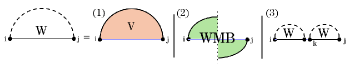
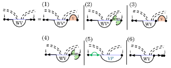
Fig. 3 illustrates this decomposition of general subproblems, which allows to calculate $W_{i,j}$ by minimizing over all possible cases. The HFold algorithm delegates the first two cases, where the substructure is closed by either a regular loop or a pseudo-loop, to additional recurrences $V_{i,j}$ and $WMB_{i,j}$ . $V_{i,j}$ refers to the MFE of the structures of the subsequence $S_{i..j}$ that contain the base pair $(i,j)$ ; $WMB_{i,j}$ refers to the MFE of the structures that contain the chain of base pairs connecting $i$ to $j$ . In all remaining cases, the optimal structure can be decomposed into the general MFE structures of a prefix $S_{i..k}$ and a suffix $S_{k+1..j}$ for some $i<k<j$ .

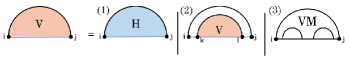
As illustrated in Fig. 4, the MFE $V_{i,j}$ of substructures closed by a regular loop, can be obtained by minimizing energies over the cases of a hairpin loop, $\mathcal{H}$ _i,j, an internal loop $\mathcal{I}$ _i,k,l,j, or a multiloop closed by $(i,j)$ , $VM_{i,j}$ .

Note that $VM_{i,j}$ accounts for branches leading into pseudoknotted substructures, yet its recurrence otherwise mirrors the pseudoknot-free formulation. Consequently, we omit its details and focus instead on $WMB_{i,j}$ , which computes the MFE when the substructure is closed by a pseudoloop, where our principal algorithmic contributions arise.

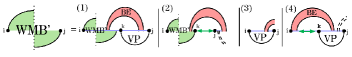
In the recurrence for $WMB_{i,j}$ , two cases arise depending on whether $j$ is paired as part of the input structure $G$ (Fig. 5): (1) $j$ forms the base pair $(j^{\prime},j)$ in $G$ , and (2) $j$ is unpaired in $G$ (or paired only in $G^{\prime}$ ). The latter is handled by the auxiliary matrix $W\!M\!B^{\prime}$ , introduced by HFold to optimize the corresponding energy.

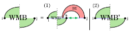
In the first case, the pair $(j^{\prime},j)$ must be crossed by another pair $(k^{\prime},k)$ in $G^{\prime}$ . Each choice of $k$ specifies a unique band in $G$ whose energy is computed in the matrix $B E$ . Removing this band leaves a prefix of the pseudoloop, whose energy is minimized with $W\!M\!B^{\prime}$ , and a substructure spanning the region between $k$ and the band around $j$ . To optimize the energy of the latter region, HFold employs the matrix $W\!I$ , which is analogous to W but uses the energy parameters specific to the interior of a pseudoloop.

When $j$ is paired in $G^{\prime}$ , the recurrence for $WMB_{i,j}$ resorts to the auxiliary matrix $W\!M\!B^{\prime}$ (Fig. 6). In its first branch, $W\!M\!B^{\prime}$ resolves the two rightmost bands with the help of BE and a new matrix $V\!P$ , then recurses on the remaining prefix of the pseudoloop. The matrix $V\!P$ , defined below, handles segments closed by a base pair that crosses pairs in $G$ , a configuration not covered by the standard $V$ matrix.

The second branch of $W\!M\!B^{\prime}$ trims a recursive substructure from the right, while the final two branches terminate the recursion, assigning the residual energy when only one or two bands remain in the pseudoloop.

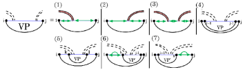
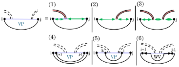
The recurrence for $V\!P$ (Fig. 7) handles three loop types that cross a band of $G$ : hairpin (cases 1-3), internal loop (cases 4 and 5) and multiloops that span the band (cases 6 and 7). These cases are broken down further based on how they cross the band(s) of $G$ . Formulating these recurrences requires an additional auxiliary matrix, $W\!I^{\prime}$ . $W\!I^{\prime}$ is similar to W and $W\!I$ , but is evaluated in the context of multiloops that span a band and, moreover, it cannot correspond to empty structures.

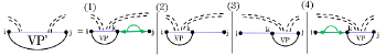
Case 6 and 7 of VP, which handle multiloops that span a band, are broken down further by the recurrence $V\!P^{\prime}$ (Fig. 8), which handles parts of a multiloop that spans a band efficiently by “consuming” recursive substructure on the right (cases 1 and 2) and the left (cases 3 and 4) of the base pair that crosses $G$ .

3 The Spark Algorithm

Recall that the presented algorithm Spark solves exactly the same problem as HFold but uses sparsification to achieve better run-time and memory performance. Because Spark follows the general recursion scheme of HFold, we focus on the novelties due to sparsification and their correctness. Recall from the introduction that we developed Spark in order to achieve the same theoretical complexities as sparsified pseudoknot-free minimum-free-energy prediction [23]. In particular, we replace the quadratic storage requirements of HFold by requiring only space for sparse data structures ( $Z$ candidates and $T$ trace arrows) and otherwise loglinear space. Notably, the space reduction by sparsification goes hand-in-hand with an improvement of the time complexity from $O(n^{3})$ to $O(n^{2}+nZ)$ , since less entries have to be considered in the linear minimizations cases.

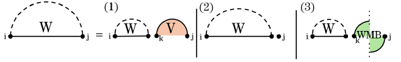
We first outline the core sparsification strategy for pseudoknot-free MFE prediction and then extend it to pseudoknotted structures. Recall that $W_{i,j}$ is computed by minimizing over two alternatives: (1) nucleotides $i$ and $j$ close a loop, handled by $V_{i,j}$ , and (2) the optimal substructure of region $[i,j]$ can be split at some index $k$ into two disjoint substructures; in this case, we obtain the best energy by minimizing over $W_{i,k-1}+W_{k,j}$ for all $k$ , $i<k\leq j$ . The latter minimization can be restricted to candidates, where $W_{k,j}$ is the energy of a closed structure (i.e. $W_{k,j}=V_{k,j}$ ) and there is no equally good (or better) way to split $[k,j]$ again. This works, since non-candidate splits can not yield a better energy than candidate splits due to $W_{i,j}\leq W_{i,k-1}+W_{k,j}$ [22, 23], formally $[i,j]$ is a candidate if and only if it is not optimally decomposable, i.e. $V_{i,j}<W_{i,k-1}+W_{k,j}$ for all $i<k\leq j$ . Consequently, the minimization of $W_{i,k-1}+W_{k,j}$ is sparsified by changing it to

\min_{\text{$i<k<j$, $[k,j]$ is a candidate}}W_{i,k-1}+V_{k,j}

and adding an extra case $W_{i,j-1}$ (“unpaired $j$ ”). In this way, we can efficiently evaluate the recurrences without storing the entire quadratic dynamic programming matrices, as long as we remember the energies $V_{i,j}$ of the candidates $[i,j]$ in a sparse data structure.

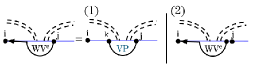
In the pseudoknotted case, $W_{i,j}$ has a third alternative, $WMB_{i,j}$ , where $i$ and $j$ close a pseudoloop. When sparsifying the split alternative, we therefore face two possibilities: (1) as in the pseudoknot-free setting, nucleotide $k$ pairs with $j$ to close a regular loop, handled by $V_{k,j}$ ; or (2) $k$ and $j$ close a pseudoloop. To distinguish these situations, we use the $W$ recurrence illustrated in Fig. 9, which strategically removes the rightmost substructure. In case (1) the rightmost substructure is a regular loop, in case (2) it is a single unpaired base, and in case (3) it is a pseudoloop. Note that cases (1) and (3) when $k=i$ correspond to the cases 1 and 2 in Fig. 3. To distinguish between the candidates, we refer to candidates for case (1) as $V$ -candidates and for case (3) as $W\!M\!B$ -candidates, and store them seperately.

When using a realistic energy model (such as HotKnots 2.0 or Turner 99), recovering the MFE structure from candidates alone is not possible [23]. To enable reconstruction, additional cells of the energy matrices, referred to as trace arrows, are kept. Trace arrows are updated regularly and removed once no longer needed by garbage collection [23].

In the following, we discuss the required novel developments of Spark for sparsifying the decomposition of pseudoloops, leading to sparse analogons of $W\!M\!B$ , $W\!M\!B^{\prime}$ , $V\!P$ and auxilliary recurrences.

We systematically rewrite the linear minimization cases of HFold in order to replace access to entries of the matrices W, $W\!I$ , and $W\!I^{\prime}$ by candidates. Since not every use of $W\!I$ can be replaced in this way, avoiding super-linear space for $W\!I$ requires specific novel data structures $W\!I$ -right and $W\!I$ -left.

3.1 The decomposition of general pseudoloops

Recall the decomposition of pseudoloops in $W\!M\!B$ (Fig. 5). Note that, in this recurrence, the access to $W\!I$ -entries cannot be avoided by restriction to candidates as described before. At the same time, storing more than a linear number of $W\!I$ entries would exceed the targeted space complexity. We solve this issue by strategically selecting the breaking point in case (1), such that we can store all required $W\!I$ substructures in linear space.

Storing all relevant WI in linear space.

In case (1) of $WMB_{i,j}$ , the subregion handled by $W\!I$ spans from index $k$ to the inner border of the rightmost band within $G_{i,j}$ . Because the input structure $G$ is fixed, this right boundary is known in advance. We leverage this property to store the relevant $W\!I$ energies efficiently using the $W\!I$ -right data structure, which is defined as follows:

$\blacksquare$

Each subregion is denoted as $[l,r]$ , where $l$ is the leftmost index and $r$ is the fixed rightmost boundary of the subregion.
$\blacksquare$

The right boundary $r$ is determined by the immediate enclosing base pair $(i,j)$ , such that $r=j-1$ .
$\blacksquare$

Within the same $W\!I$ region, no two $W\!I$ -right subregions overlap.

These conditions ensure that $W\!I$ -right partitions $W\!I$ into distinct, non-overlapping subregions, each corresponding to a nested disjoint substructure with a clearly defined right boundary set by its parent base pair.

Lemma 1.

The linear-space data structure $W\!I$ -right is sufficient to compute all relevant $W\!I$ cases in $W\!M\!B$ .

Proof.

Recall that $WMB_{i,j}$ case 1 requires the computation of terms of the form $W\!M\!B^{\prime}$ $(i,k-1)+$ $W\!I$ $(k,B^{\prime})$ , where $B^{\prime}$ is the rightmost inner band border of $G_{i,j}$ . The goal is to store all potentially relevant $W\!I$ values in linear space. If the regions covered by $W\!I$ -right entries do not overlap, linear storage is achievable.

We demonstrate by contradiction that no overlap between these regions is possible. Suppose, for contradiction, that there is an overlap between two regions stored in $W\!I$ -right. Specifically, assume base pairs $(i,j)$ and $(k,l)$ exist, with $(k,l)$ nested within $(i,j)$ , and assume an overlap between their corresponding $W\!I$ -right regions. Then there must exist some position $m$ that simultaneously defines two weakly closed regions: $[m,l-1]$ and $[m,j-1]$ . Consider the two possible positions for such an overlapping point $m$ : $m=m_{1}$ or $m=m_{2}$ , as illustrated in Fig. 10.

$\blacksquare$

If $m=m_{1}$ , the overlapping region would be $[m,k-1]$ . However, by definition, for a region $[x,y]$ to be valid for a $W\!I$ calculation, it must form a weakly closed region (i.e. no base inside the region pairs with a base outside of the region) in which the immediate base pair covering $x$ and $y$ are the same (referred to as $cover(x)=cover(y)$ ). Here, region $[m,l-1]$ fails to satisfy this condition (as $cover(m)\neq cover(l-1)$ ), contradicting its existence as a valid region.
$\blacksquare$

Similarly, if $m=m_{2}$ , the overlapping region would occur within $[m,l-1]$ and $[m,j-1]$ . Again, region $[m,j-1]$ does not satisfy the weakly closed condition ( $cover(m)\neq cover(j-1)$ ), contradicting the assumption that it is a valid region.

Since both cases lead to contradictions, no such overlapping regions exist. Hence, the data structure $W\!I$ -right requires only linear space to store all relevant $W\!I$ cases. $\hfill\blacktriangleleft$

3.2 Decomposition of pseudoloops with rightmost band in $G^{\prime}$

To handle the prefixes of pseudoloops, where the rightmost position is not paired in $G$ , we rewrite the $W\!M\!B^{\prime}$ recurrence (Fig. 6) following the general idea of replacing access to $W\!I$ with candidates. For this purpose, we introduce the recurrence $W\!M\!B^{\textrm{A}}$ .

As illustrated in Fig. 11, cases (1) and (3) recursively consume the substructure formed by $j$ and its paired nucleotide; this is computed by $V\!P$ . Similar to selecting positions $k$ during sparsification of W, we restrict our choice of $k$ here to those for which the region $[k,j]$ is a valid candidate (precisely, a $V\!P$ -candidate). Case (2) represents a terminal case.

$W\!M\!B^{\textrm{A}}$ recursively consumes the rightmost nested substructure. As illustrated in Fig. 12, case (1) handles the scenario where position $j$ is unpaired. Case (2) deals with the rightmost nested $V$ substructure within $[i,j]$ , while case (3) handles the rightmost nested $W\!M\!B$ substructure within $[i,j]$ . Finally, case (4) recurses back to $W\!M\!B^{\prime}$ to continue consuming additional portions of the pseudoloop. Note that in cases (2) and (3), we only consider substructures $V_{k,j}$ and $WMB_{k,j}$ for which the region $[k,j]$ is a valid candidate.

In the following lemma, we demonstrate that the revised recurrences for $W\!M\!B^{\prime}$ and $W\!M\!B^{\textrm{A}}$ together correctly cover all cases originally handled by the $W\!M\!B^{\prime}$ recurrence.

Lemma 2.

Replacing the original $W\!M\!B^{\prime}$ recurrence with the revised $W\!M\!B^{\prime}$ and the newly defined $W\!M\!B^{\textrm{A}}$ recurrences is both complete and correct.

Proof.

The original recurrence for $W\!M\!B^{\prime}$ _i,j, depicted in Fig. 6, includes four cases, with case (2) recursively trimming a substructure from the right using the $W\!I$ matrix. The revised recurrence for $W\!M\!B^{\prime}$ _i,j retains the original cases (1), (3), and (4), while delegating the handling of case (2) to the newly introduced $W\!M\!B^{\textrm{A}}$ recurrence. The $W\!M\!B^{\textrm{A}}$ recurrence explicitly addresses the distinct sub-cases previously embedded within the $W\!I$ recursion and employs sparsification to enhance efficiency.

By comparing the original definition in Fig. 6 with the revised definitions in Figures 11 and 12, we confirm that all original cases are accounted for, establishing the completeness and correctness of the revised formulation. $\hfill\blacktriangleleft$

3.3 Prediction of closed structures that cross $𝑮$

Recall that HFold decomposed crossing closed structures by $V\!P$ (Fig. 7). $V\!P$ $(i,j)$ is the minimization over all structures $R_{i,j}$ in which $(i,j)\in G^{\prime}$ and crosses a base pair in $G$ . If $i\geq j$ , $i$ or $j$ is paired in $G$ , or $(i,j)$ does not cross any base pair of $G$ , then $V\!P$ $(i,j)=\infty$ . We have updated the recurrences accordingly for sparsification. Fig. 13 illustrates the updated cases.

Cases (1)-(3) of our updated $V\!P$ follow the same logic as in the original $V\!P$ . Under the assumption that there are no other base pairs within $[i,j]$ that intersect the same bands as $(i,j)$ , cases (1)-(3) handle the nested substructures within. The nested substructures are broken down by the $W\!I$ recurrence (see supplementary material).

Storing all relevant WI in linear space.

In cases (1)-(3) of our revised $V\!P$ recurrence (similar to case (1) of the previously discussed the updated $W\!M\!B^{\prime}$ ), the subregions handled by $W\!I$ extend either from the inner border of a left band or the outer border of a right band within $G_{i,j}$ . Because the input structure $G$ is fixed, these left boundaries are known in advance. Analogous to our approach with $W\!I$ -right, we exploit this property to efficiently store the relevant $W\!I$ energies using a dedicated data structure called the $W\!I$ -left data structure, defined as follows:

$\blacksquare$

Each subregion is represented as $[l,r]$ , where $l$ denotes the fixed left boundary and $r$ is the rightmost position of the subregion.
$\blacksquare$

The left boundary $l$ is determined either by the immediately enclosing base pair $(i,j)$ (thus $l=i+1$ ), or by another enclosing base pair $(k,m)$ (thus $l=m+1$ ).
$\blacksquare$

Although multiple $W\!I$ -left subregions within the same $W\!I$ region may overlap spatially, their use-cases remain non-overlapping.

Lemma 3.

The linear data structure $W\!I$ -left is sufficient to calculate all relevant $W\!I$ cases in $W\!M\!B^{\prime}$ and $V\!P$ .

Proof.

The proof follows similar reasoning to that of Lemma 1 for the $W\!I$ -right case. Specifically, we proceed by contradiction to demonstrate that there are no overlapping use-cases among the regions encompassed by $W\!I$ -left. This ensures that the $W\!I$ -left data structure can be stored efficiently in linear space. $\hfill\blacktriangleleft$

In case (6) of the revised $V\!P$ recurrences $(i,j)$ closes a multiloop that spans a band. Within this substructure, one band of the multiloop crosses the same band in $G$ as $(i,j)$ , while the remaining bands and unpaired bases are processed as nested substructures through the $W\!I^{\prime}$ recurrence. In the Original $V\!P$ recurrence – see Fig. 7 – cases (6) and (7) handled the decomposition by either breaking off a non-empty region on the left or right via $W\!I$ and decomposing the rest through the $V\!P^{\prime}$ recurrence – see Fig. 8. As the regions of $W\!I$ , which occur within both $V\!P$ and $V\!P^{\prime}$ , are not contiguous with a band boundary, this would not have been solvable through sparsification in the original recurrences. We instead define a new recurrence, $W V$ to handle this substructure which we illustrate in Fig. 14. Specifically, $WV_{i,j}$ is the MFE of all valid structures $R_{i,j}$ over region $[i,j]$ given that $[i,j]$ is not weakly closed (i.e. one base in the region pairs with a base outside of the region) and contains at least two inner base pairs where one is a $V\!P$ . $W V$ represents the fragments of a multiloop that spans a band. A multiloop spanning a band can be decomposed into three cases: empty on the left side, empty on the right side, or non-empty on both sides. Since we must guarantee that at least one side contains a substructure and that $W\!I^{\prime}$ cannot represent an empty region, we use $W\!V^{\textrm{e}}$ to handle cases that are empty on the left but non-empty on the right. Figure 14 illustrates these cases.

Cases (1) and (2) address scenarios in which the left side of the multiloop that spans a band is empty. To ensure that these cases result in a valid multiloop, the right side must contain either a candidate $V$ or $W\!M\!B$ substructure (both involving $j$ ). Cases (3) and (4) handle situations where multiple base pairs exist on the right side. In these scenarios, the right-side region is segmented to accommodate these base pairs. Because the energy computation depends on $WV_{i,k-1}$ , one of the previous cases must also apply. We apply sparsification in both these cases and only consider breaking points that result in candidates. Case (5) covers scenarios in which the left side of the multiloop that spans a band consists of a closed region. Since this condition does not impose additional constraints on the right side, it allows either unpaired bases or another closed region. Finally, case (6) accounts for situations involving an unpaired nucleotide on the right side.

Intuitively, cases 1, 2, and 5 represent terminal cases. In contrast, cases 3, 4, and 6 allow the right region to be recursively decomposed until a terminal case is encountered.

To satisfy the conditions for multiloops in cases where the left region is empty (i.e. case (1) and (2)), we have to ensure that the structure on the right is not empty. For this reason, we define the recurrence $W\!V^{\textrm{e}}$ , which handles structures that have unpaired bases on the left and an interior base pair spanning the band. Notably, we apply this recurrence only when the right side of the multiloop contains at least one base pair.

Formally, $W\!V^{\textrm{e}}_{i,j}$ denotes the MFE of all valid structures $R_{i,j}$ within the region $[i,j]$ , given that $[i,j]$ is not weakly closed. Specifically, $W\!V^{\textrm{e}}$ characterizes multiloop fragments spanning a band where the left side consists entirely of unpaired bases. Note that in case (1) we utilize sparsification and only consider breaking points $k$ for which $[k,j]$ is a $V\!P$ -candidate. Figure 15 illustrates $W\!V^{\textrm{e}}$ recurrence.

Lemma 4.

The combined recurrences $W V$ and $W\!V^{\textrm{e}}$ cover exactly the cases handled by the original recurrences of $V\!P^{\prime}$ .

Proof.

A multiloop spanning a band can be decomposed into exactly three scenarios:

(1)

A paired region on the left, a band in the middle, and a paired region on the right.
(2)

A paired region on the left, a band in the middle, and an empty region on the right.
(3)

An empty region on the left, a band in the middle, and a paired region on the right.

The original recurrences for $V\!P$ and $V\!P^{\prime}$ , illustrated in Fig. 7 and Fig. 8, handle these scenarios as follows:

$\blacksquare$

Case 6 of $V\!P$ considers scenarios (1) and (2).
$\blacksquare$

Case 7 of $V\!P$ considers scenarios (1) and (3).
$\blacksquare$

The resulting decomposition from $V\!P$ is further detailed by $V\!P^{\prime}$ , explicitly addressing all three scenarios.

We verify now that each of these three scenarios is fully represented by our updated recurrences $W V$ and $W\!V^{\textrm{e}}$ :

$\blacksquare$

Scenario (1): Paired regions on both sides. Cases 3–6 of $W V$ explicitly handle paired structures on both the left and right sides. Cases 3,4, and 6 recursively decompose the right side until the structure reduces to a single paired region on the left and a band in the middle, which is then covered by case 5 of $W V$ .
$\blacksquare$

Scenario (2): Paired region on the left, empty region on the right. This scenario is handled by cases 5 and 6 of $W V$ . Case 6 recursively decomposes any unpaired bases on the right until the structure simplifies to a single paired region on the left and an adjacent empty region on the right. This simpler configuration is then directly managed by case 5 of $W V$ .
$\blacksquare$

Scenario (3): Empty region on the left, paired region on the right. This case is managed by cases 1–4,and 6 of $W V$ . If the right side has exactly one paired structure, we directly transition into the $W\!V^{\textrm{e}}$ recurrence using cases 1–2. If multiple paired structures exist on the right, cases 3,4, and 6 recursively decompose them until a single remaining paired structure allows entry into $W\!V^{\textrm{e}}$ through cases 1–2. Importantly, $W\!V^{\textrm{e}}$ ensures that a valid paired structure is indeed present on the right side (required due to the left side being empty), and it explicitly considers scenarios where unpaired bases might separate the band from the right-side paired structure.

As all scenarios originally covered by $V\!P$ and $V\!P^{\prime}$ are systematically addressed, the combination of $W V$ and $W\!V^{\textrm{e}}$ fully and correctly captures these cases. $\hfill\blacktriangleleft$

3.4 Time and Space Complexity

After sparsification, Spark achieves efficient bounds in both time and space. Recall that $n$ denote the sequence length, $Z$ the total number of candidate intervals retained by sparsification, and $T$ the number of trace arrows stored for back-tracing the MFE structure.

Space complexity.

The memory footprint of Spark is the sum of three subquadratic-sized components:

1.

Sequence array – the input RNA string and the array holding structure information requires $O(n)$ and $O(n\log(n))$ space (following an efficient implementation of sparse tree to keep the band border information).
2.

Candidate lists – sparsification keeps values only for intervals that can participate in an optimal solution. Lemma 1 and its symmetric analogue for $W\!I$ -left guarantee that every position is contained in at most one active $W\!I$ region of each type, so all candidate tables together use $O(Z)$ space, where $Z<<n^{2}$ typically.
3.

Trace arrows – each stored sub-solution carries at most one predecessor pointer; therefore the total number of arrows is $O(T)$ .

No other data structure grows with either $n$ or $Z$ , giving the overall memory bound $O(n\log(n)+Z+T)$ .

Time complexity.

The running time combines a quadratic baseline over all position pairs with a linear scan of candidates per left index:

$\blacksquare$

Constant-bounded internal loops. Each dynamic-programming recurrence considers internal loops of size at most 30 – a standard cut-off.
$\blacksquare$

Candidate-driven scanning. For every fixed left index $i$ we test at most $Z$ candidate intervals $[k,j]$ that start at $i$ . The outer loop over $i$ therefore adds $n\times Z=O(nZ)$ steps.

Combining both parts yields the total running time $O(n^{2}+nZ)$ .

4 Experimental Design

4.1 Dataset

We used the original dataset from SparseMFEFold [23], consisting of $3704$ RNA sequences categorized into $6$ distinct families, sourced from the RNAstrand V2.0 database [1]. These sequences range in length from $8$ to $4381$ nucleotides.

Constraint structures were generated by randomly selecting pairs of indices within each sequence. If the chosen bases could pair and were separated by at least 3 nucleotides, the base pair was extended via stacking interactions to form the maximal stem. Among these stems, the one with the lowest energy was selected as the constraint structure. To allow for potential long-range interactions, including multiloops or pseudoknots, the energy of the innermost base pair was set to $0$ .

To expand the dataset and evaluate longer sequences, we included the SARS-CoV-2 genome (length $29903$ nucleotides) with a constraint structure derived previously [26, 25]. This constraint structure was obtained by combining all non-overlapping stems to yield the minimal free-energy constraint structure. Additionally, to systematically examine sequences of increasing length, partial segments of the SARS-CoV-2 genome were extracted, beginning from length $4000$ nucleotides and incrementally increasing by $2000$ nucleotides up to the full-length genome.

4.2 Energy Model

In Spark, we employ the DP09 parameter set from HotKnots 2.0 – an update to the earlier DP03 model that was trained on a large set of experimentally validated pseudoknotted structures [2]. The pseudoknotted parameter list appears in Supplementary Table 1.

5 Results

5.1 Spark and HFold compute identical energies on crossing structures

We validated the implementation of Spark by comparing its results against the HFold implementation on our dataset. Spark and HFold predicted identical MFE values across all test cases. As expected, since the optimal structures are not necessarily unique, the tools report different optimal structures in few cases. Detailed results of this comparison are available in our repository.

5.2 Spark’s empirical time and space outperforms HFold and closely matches RNAfold

We assessed the empirical time and memory requirements of Spark and compared them with those of RNAfold and HFold. RNAfold– a highly optimised, pseudoknot-free algorithm – provides a practical lower bound: matching or approaching its performance demonstrates that Spark ’s sparsification effectively offsets the extra cost of pseudoknot prediction. HFold, which also predicts hierarchically constrained pseudoknots but is not sparsified, serves as the natural unsparsified reference.

All experiments were run on an M2 Max Mac Studio with 64 GB of RAM. Runtimes were recorded as user CPU time (Fig.16a) and memory usage as maximum resident set size (Fig. 16b). Because constrained pseudoknot prediction requires an input scaffold, every algorithm – including RNAfold– received the same partial structure for each sequence. For all sequences we selected the minimum-free-energy stem-loop as described in section 4.1, ensuring a fair comparison.

HFold can process only sequences shorter than 5000 nt, so it was evaluated solely on the original SparseMFEFold dataset [23]. On this set, HFold ’s maximum runtime and memory footprint were 31,047 s and 937 MB. By contrast, RNAfold required at most 12.8 s and 106 MB, while Spark needed just 15.7 s and 35.8 MB.

To highlight the impact of sparsification on longer RNAs, we extended the dataset as detailed in section 4.1. The largest sequence, the complete SARS-CoV-2 genome (29903 nt), is beyond HFold ’s range. RNAfold processed this genome in 2,927 s using 4.81 GB of memory; Spark completed in 2,869 s with only 1.43 GB. Results for all sequences are summarised in Fig. 16.

These experiments demonstrate that Spark maintains pseudoknot-handling capability while using substantially less memory than either comparator and achieving runtimes comparable to the pseudoknot-free RNAfold even on the largest sequences tested.

Figure 16: We plot the results of Spark against two state of the art algorithms: HFold and RNAfold when given an RNA sequence and input structure only as input against each other on our dataset. (a) Run-time (s) versus length (log-log plot) over all benchmark instances. For each tool in both plots, we report (in parenthesis) the exponent x that we estimated from the benchmark results; it describes the observed complexity as

\Theta(n^{x})

. (b) Memory Usage (maximum resident set size in KB) versus length (log-log plot) over all benchmark instances. The solid line shows an asymptotic fit

(c1+c2n^{x})

for sequence length n, constants c1,c2, and exponent x for the fit. We ignored all values

<

1000.

5.3 Effect of Pseudoknot Parameters on Candidate Growth

Sparsification inevitably increases the number of candidate intervals when the recurrence system is extended from pseudoknot-free to pseudoknotted prediction. Figure 17 quantifies this effect for the entire test set, including the full SARS-CoV-2 genome ( $n=29,903$ ) and its subsequences.

The input constraint structure is the primary determinant of how many intervals survive sparsification; nevertheless, the energy parameters also matter. Switching to pseudoknot recurrences introduces harsher unpaired-base penalties inside pseudoloops, so base pairs that minimise the number of unpaired bases become energetically preferable. As a result, additional $V$ -candidates (and their associated trace arrows) must be kept because they participate in $W\!I$ and $W\!I^{\prime}$ computations (cf. SparseRNAFolD [9] for the analogous rules in the pseudoknot-free case).

Empirically, the growth is moderate: on our largest sequences we observe at most a four-fold increase in $V$ -candidates and a two-fold increase in $V$ trace arrows relative to the pseudoknot-free setting. Crucially, the total number of candidates and trace pointers grows strictly slower than a quadratic function, slightly deviating from a linear growth. Figure 17 plots these counts alongside the $n^{2}$ curve for a full quadratic matrix; even for the 30 kb SARS-CoV-2 genome the candidate count remains well below the quadratic envelope. These results confirm that extending the model to pseudoknots increases the search space, but not to the point of negating the asymptotic advantages of sparsification.

Figure 17: We plot the V candidates and trace arrows of the standard Spark against the PKfree, when given the same input.

6 Conclusion

In this work we present Spark, a biologically-motivated, sparsified algorithm that applies the hierarchical-folding hypothesis to compute the MFE structure of an RNA sequence given a pseudoknot-free input structure as constraint. By integrating sparsification into every dynamic-programming table as explained above, Spark reduces the effective search space to a small set of candidates. Formally, for a sequence of length $n$ , let $Z$ be the number of candidates, and $T$ the number of trace arrows required to reconstruct the optimal structure. We show (see the complexity argument above) that Spark runs in $O(n^{2}+nZ)$ time and $O(n\log(n)+Z+T)$ space, improving on the $O(n^{3})$ time and $O(n^{2})$ space bounds of the original hierarchical algorithm HFold. In typical datasets, $Z$ grows close to linearly with $n$ , so the practical cost approaches quadratic time and loglinear space.

Empirical evaluation.

We benchmarked Spark against the unsparsified HFold and the highly optimised, pseudoknot-free RNAfold on a collection of 3704 RNA sequences drawn from six RNA families, augmented with partial and full SARS-CoV-2 genomes (up to 29903 nt). On the SparseMFEFold set – where HFold can still be run – Spark required at most 15.7 s and 35.8 MB, compared with 31047 s and 917 MB for HFold and 12.8 s and 106 MB for RNAfold. On the full SARS-CoV-2 genome, Spark finished in 2869 s using 1.43 GB, while RNAfold needed 2927 s and 4.81 GB; HFold cannot handle sequences of this length at all.

Practical impact.

Efficient sparsification allows Spark to predict hierarchically-constrained pseudoknotted structures in RNA sequences exceeding 30000 nt – a regime previously out of reach for MFE-based methods. This capability opens the door to routine large-genome analyses, such as coronavirus or plant-viral RNAs, while retaining the theoretical guarantees of exact dynamic programming.

References

[1] Mirela Andronescu, Vera Bereg, Holger H Hoos, and Anne Condon. RNA STRAND: The RNA secondary structure and statistical analysis database. BMC Bioinformatics, 9(1):340+, August 2008. doi:10.1186/1471-2105-9-340.
[2] Mirela S Andronescu, Cristina Pop, and Anne E Condon. Improved free energy parameters for RNA pseudoknotted secondary structure prediction. RNA, 16(1):26–42, 2010.
[3] Rolf Backofen, Dekel Tsur, Shay Zakov, and Michal Ziv-Ukelson. Sparse RNA folding: Time and space efficient algorithms. Journal of Discrete Algorithms, 9:12–31, March 2011. doi:10.1016/j.jda.2010.09.001.
[4] José A Cruz and Eric Westhof. The dynamic landscapes of RNA architecture. Cell, 136:604–609, February 2009. doi:10.1016/j.cell.2009.02.003.
[5] Robert M Dirks and Niles A Pierce. A partition function algorithm for nucleic acid secondary structure including pseudoknots. Journal of Computational Chemistry, 24:1664–1677, August 2003. doi:10.1017/s1355838298980116.
[6] Andreas Gruber et al. The Vienna RNA websuite. Nucleic Acids Res, 36:W70–W74, July 2008. doi:10.1093/nar/gkn188.
[7] Raheleh Salari et al. Time and space efficient RNA-RNA interaction prediction via sparse folding. In Lecture Notes in Computer Science, volume 6044, pages 473–490. Research in Computational Molecular Biology, 2010. doi:10.1007/978-3-642-12683-3_31.
[8] Mateo Gray, Sebastian Will, and Hosna Jabbari. Spark. Software, swhId: swh:1:dir:2cb07371af448bb6254c05d23ac106800c590d39 (visited on 2025-08-05). URL: https://github.com/TheCOBRALab/Spark, doi:10.4230/artifacts.24328.
[9] Mateo Gray, Sebastian Will, and Hosna Jabbari. SparseRNAfolD: optimized sparse RNA pseudoknot-free folding with dangle consideration. Algorithms Mol Biol, 19(9):26–42, 2024.
[10] Hosna Jabbari and Anne Condon. A fast and robust iterative algorithm for prediction of RNA pseudoknotted secondary structures. BMC Bioinformatics, 15, May 2014. doi:10.1186/1471-2105-15-147.
[11] Hosna Jabbari, Anne Condon, Ana Pop, Christina Pop, and Yinglei Zhao. Hfold: RNA pseudoknotted secondary structure prediction using hierarchical folding. In Raffaele Giancarlo and Sridhar Hannenhalli, editors, Algorithms in Bioinformatics, pages 323–334, Berlin, Heidelberg, 2007. Springer Berlin Heidelberg. doi:10.1007/978-3-540-74126-8_30.
[12] Hosna Jabbari, Anne Condon, and Shelly Zhao. Novel and efficient RNA secondary structure prediction using hierarchical folding. J. Comput. Biol., 15(2):139–163, March 2008. doi:10.1089/cmb.2007.0198.
[13] Hosna Jabbari, Ian Wark, Carlo Montemagno, and Sebastian Will. Sparsification Enables Predicting Kissing Hairpin Pseudoknot Structures of Long RNAs in Practice. In 17th International Workshop on Algorithms in Bioinformatics (WABI 2017), volume 88 of Leibniz International Proceedings in Informatics (LIPIcs), pages 12:1–12:13. Schloss Dagstuhl – Leibniz-Zentrum für Informatik, 2017. doi:10.4230/LIPIcs.WABI.2017.12.
[14] Hosna Jabbari, Ian Wark, Carlo Montemagno, and Sebastian Will. Knotty: efficient and accurate prediction of complex RNA pseudoknot structures. Bioinformatics, 34:3849–3856, November 2018. doi:10.1093/bioinformatics/bty420.
[15] Marilyn Kozak. Regulation of translation via mRNA structure in prokaryotes and eukaryotes. Gene, 361:13–37, November 2005. doi:10.1016/j.gene.2005.06.037.
[16] David H Matthews, Matthew D Disney, Jessica L Childs, Susan J Schroeder, Michael Zuker, and Douglas H Turner. Incorporating chemical modification constraints into a dynamic programming algorithm for prediction of RNA secondary structure. Proceeding of the National Academy of Science of the USA, 101:7287–7292, May 2004. doi:10.1073/pnas.0401799101.
[17] Stephanie A Mortimer, Mary A Kidwell, and Jennifer A Doudna. Insights into RNA structure and function from genome-wide studies. Nature Reviews Genetics, 15:469–479, May 2014. doi:10.1038/nrg3681.
[18] Jihong Ren, Baharak Rastegari, Anne Condon, and Holger H Hoos. HotKnots: Heuristic prediction of RNA secondary structures including pseudoknots. RNA, 11:1494–1504, October 2005. doi:10.1261/rna.7284905.
[19] Jihong Ren, Baharak Rastegari, Anne Condon, and Holger H Hoos. Hotknots: heuristic prediction of RNA secondary structures including pseudoknots. RNA, 11(10):1494–1504, 2005.
[20] Elena Rivas and Sean R Eddy. A dynamic programming algorithm for rna structure prediction including pseudoknots. Journal of Molecular Biology, 285:2053–2068, February 1999. doi:10.1006/jmbi.1998.2436.
[21] Bryan M Warf and Andrew J Berglund. Role of RNA structure in regulating pre-mRNA splicing. Trends Biochem Sci., 35:169–178, March 2010. doi:10.1016/j.tibs.2009.10.004.
[22] Ydo Wexler, Chaya Zilberstein, and Michal Ziv-Ukelson. A study of accessible motifs and RNA folding complexity. Journal of Computational Biology, 14:856–872, August 2007. doi:10.1089/cmb.2007.R020.
[23] Sebastian Will and Hosna Jabbari. Sparse RNA folding revisited: space-efficient minimum free energy structure prediction. Algorithms for Molecular Biology, 11, April 2016. doi:10.1186/s13015-016-0071-y.
[24] Timothy J Wilson and David M J Lilley. RNA catalysis—is that it? RNA, 21:534–537, April 2015. doi:10.1261/rna.049874.115.
[25] Alison Ziesel and Hosna Jabbari. Structural impact of synonymous mutations in six sars-cov-2 variants of concern. bioRxiv, 2024.
[26] Alison Ziesel and Hosna Jabbari. Unveiling hidden structural patterns in the sars-cov-2 genome: Computational insights and comparative analysis. Plos one, 19(4), 2024.

Appendix A Definitions

Table 1: ENERGY PARAMETERS. All parameters were derived at 37 degrees celsius and 1 M salt (NaCl) concentration or extrapolated from experimental values cf. [12, 2, 19].

Name	Description	Value (kcal/mol)
$P_{s}$	Exterior pseudoloop initiation penalty	-1.38
$P_{sm}$	Penalty for introducing pseudoknot inside a multiloop	10.07
$P_{sp}$	Penalty for introduce pseudoknot inside a pseudoloop	15.00
$P_{b}$	Band penalty	2.46
$P_{up}$	Penalty for unpaired base in a pseudoloop	0.06
$P_{ps}$	Penalty for closed subregion inside a pseudoloop	0.96
$e_{H}(i,j)$	Energy of a hairpin loop closed by $(i,j)$
$e_{S}(i,i+1,j-1,j)$	Energy of a stacked pair closed by $(i,j)$
$e_{stP}(i,i+1,j-1,j)$	Energy of a stacked pair that spans a band	$0.89\times e_{S}(i,j)$
$e_{int}(i,r,r^{\prime},j)$	Energy of a pseudoknot-free internal loop
$e_{intP}(i,r,r^{\prime},j)$	Energy of an internal loop that spans a band	$0.74\times e_{int}(i,d,e,j)$
$a$	Multiloop initiation penalty	3.39
$b$	Multiloop base pair penalty	0.03
$c$	Penalty for unpaired base in a multiloop	0.02
$a^{\prime}$	Penalty for introducing a multiloop that spans a band	3.41
$b^{\prime}$	Base pair penalty for a multiloop that spans a band	0.56
$c^{\prime}$	Penalty for unpaired base in a multiloop that spans a band	0.12

[bib.bib1] [1] Mirela Andronescu, Vera Bereg, Holger H Hoos, and Anne Condon. RNA STRAND: The RNA secondary structure and statistical analysis database. BMC Bioinformatics, 9(1):340+, August 2008. doi:10.1186/1471-2105-9-340.

[bib.bib2] [2] Mirela S Andronescu, Cristina Pop, and Anne E Condon. Improved free energy parameters for RNA pseudoknotted secondary structure prediction. RNA, 16(1):26–42, 2010.

[bib.bib3] [3] Rolf Backofen, Dekel Tsur, Shay Zakov, and Michal Ziv-Ukelson. Sparse RNA folding: Time and space efficient algorithms. Journal of Discrete Algorithms, 9:12–31, March 2011. doi:10.1016/j.jda.2010.09.001.

[bib.bib4] [4] José A Cruz and Eric Westhof. The dynamic landscapes of RNA architecture. Cell, 136:604–609, February 2009. doi:10.1016/j.cell.2009.02.003.

[bib.bib5] [5] Robert M Dirks and Niles A Pierce. A partition function algorithm for nucleic acid secondary structure including pseudoknots. Journal of Computational Chemistry, 24:1664–1677, August 2003. doi:10.1017/s1355838298980116.

[bib.bib6] [6] Andreas Gruber et al. The Vienna RNA websuite. Nucleic Acids Res, 36:W70–W74, July 2008. doi:10.1093/nar/gkn188.

[bib.bib7] [7] Raheleh Salari et al. Time and space efficient RNA-RNA interaction prediction via sparse folding. In Lecture Notes in Computer Science, volume 6044, pages 473–490. Research in Computational Molecular Biology, 2010. doi:10.1007/978-3-642-12683-3_31.

[bib.bib8] [8] Mateo Gray, Sebastian Will, and Hosna Jabbari. Spark. Software, swhId: swh:1:dir:2cb07371af448bb6254c05d23ac106800c590d39 (visited on 2025-08-05). URL: https://github.com/TheCOBRALab/Spark, doi:10.4230/artifacts.24328.

[bib.bib9] [9] Mateo Gray, Sebastian Will, and Hosna Jabbari. SparseRNAfolD: optimized sparse RNA pseudoknot-free folding with dangle consideration. Algorithms Mol Biol, 19(9):26–42, 2024.

[bib.bib10] [10] Hosna Jabbari and Anne Condon. A fast and robust iterative algorithm for prediction of RNA pseudoknotted secondary structures. BMC Bioinformatics, 15, May 2014. doi:10.1186/1471-2105-15-147.

[bib.bib11] [11] Hosna Jabbari, Anne Condon, Ana Pop, Christina Pop, and Yinglei Zhao. Hfold: RNA pseudoknotted secondary structure prediction using hierarchical folding. In Raffaele Giancarlo and Sridhar Hannenhalli, editors, Algorithms in Bioinformatics, pages 323–334, Berlin, Heidelberg, 2007. Springer Berlin Heidelberg. doi:10.1007/978-3-540-74126-8_30.

[bib.bib12] [12] Hosna Jabbari, Anne Condon, and Shelly Zhao. Novel and efficient RNA secondary structure prediction using hierarchical folding. J. Comput. Biol., 15(2):139–163, March 2008. doi:10.1089/cmb.2007.0198.

[bib.bib13] [13] Hosna Jabbari, Ian Wark, Carlo Montemagno, and Sebastian Will. Sparsification Enables Predicting Kissing Hairpin Pseudoknot Structures of Long RNAs in Practice. In 17th International Workshop on Algorithms in Bioinformatics (WABI 2017), volume 88 of Leibniz International Proceedings in Informatics (LIPIcs), pages 12:1–12:13. Schloss Dagstuhl – Leibniz-Zentrum für Informatik, 2017. doi:10.4230/LIPIcs.WABI.2017.12.

[bib.bib14] [14] Hosna Jabbari, Ian Wark, Carlo Montemagno, and Sebastian Will. Knotty: efficient and accurate prediction of complex RNA pseudoknot structures. Bioinformatics, 34:3849–3856, November 2018. doi:10.1093/bioinformatics/bty420.

[bib.bib15] [15] Marilyn Kozak. Regulation of translation via mRNA structure in prokaryotes and eukaryotes. Gene, 361:13–37, November 2005. doi:10.1016/j.gene.2005.06.037.

[bib.bib16] [16] David H Matthews, Matthew D Disney, Jessica L Childs, Susan J Schroeder, Michael Zuker, and Douglas H Turner. Incorporating chemical modification constraints into a dynamic programming algorithm for prediction of RNA secondary structure. Proceeding of the National Academy of Science of the USA, 101:7287–7292, May 2004. doi:10.1073/pnas.0401799101.

[bib.bib17] [17] Stephanie A Mortimer, Mary A Kidwell, and Jennifer A Doudna. Insights into RNA structure and function from genome-wide studies. Nature Reviews Genetics, 15:469–479, May 2014. doi:10.1038/nrg3681.

[bib.bib18] [18] Jihong Ren, Baharak Rastegari, Anne Condon, and Holger H Hoos. HotKnots: Heuristic prediction of RNA secondary structures including pseudoknots. RNA, 11:1494–1504, October 2005. doi:10.1261/rna.7284905.

[bib.bib19] [19] Jihong Ren, Baharak Rastegari, Anne Condon, and Holger H Hoos. Hotknots: heuristic prediction of RNA secondary structures including pseudoknots. RNA, 11(10):1494–1504, 2005.

[bib.bib20] [20] Elena Rivas and Sean R Eddy. A dynamic programming algorithm for rna structure prediction including pseudoknots. Journal of Molecular Biology, 285:2053–2068, February 1999. doi:10.1006/jmbi.1998.2436.

[bib.bib21] [21] Bryan M Warf and Andrew J Berglund. Role of RNA structure in regulating pre-mRNA splicing. Trends Biochem Sci., 35:169–178, March 2010. doi:10.1016/j.tibs.2009.10.004.

[bib.bib22] [22] Ydo Wexler, Chaya Zilberstein, and Michal Ziv-Ukelson. A study of accessible motifs and RNA folding complexity. Journal of Computational Biology, 14:856–872, August 2007. doi:10.1089/cmb.2007.R020.

[bib.bib23] [23] Sebastian Will and Hosna Jabbari. Sparse RNA folding revisited: space-efficient minimum free energy structure prediction. Algorithms for Molecular Biology, 11, April 2016. doi:10.1186/s13015-016-0071-y.

[bib.bib24] [24] Timothy J Wilson and David M J Lilley. RNA catalysis—is that it? RNA, 21:534–537, April 2015. doi:10.1261/rna.049874.115.

[bib.bib25] [25] Alison Ziesel and Hosna Jabbari. Structural impact of synonymous mutations in six sars-cov-2 variants of concern. bioRxiv, 2024.

[bib.bib26] [26] Alison Ziesel and Hosna Jabbari. Unveiling hidden structural patterns in the sars-cov-2 genome: Computational insights and comparative analysis. Plos one, 19(4), 2024.

Spark: Sparsified Hierarchical Energy Minimization of RNA Pseudoknots

Abstract

Motivation.

Results.

Conclusion.

Availability.

Keywords and phrases:

Copyright and License:

2012 ACM Subject Classification:

Supplementary Material:

DOI:

Event:

Editors:

Series and Publisher:

1 Introduction

Exact and accurate pseudoknot prediction.

Contributions.

Further remarks on sparsification.

2 Review of hierarchical pseudoknot prediction in HFold

3 The Spark Algorithm

3.1 The decomposition of general pseudoloops

Storing all relevant WI in linear space.

Lemma 1.

Proof.

3.2 Decomposition of pseudoloops with rightmost band in 𝑮′

Lemma 2.

Proof.

3.3 Prediction of closed structures that cross 𝑮

Storing all relevant WI in linear space.

Lemma 3.

Proof.

Lemma 4.

Proof.

3.4 Time and Space Complexity

Space complexity.

Time complexity.

4 Experimental Design

4.1 Dataset

4.2 Energy Model

5 Results

5.1 Spark and HFold compute identical energies on crossing structures

5.2 Spark’s empirical time and space outperforms HFold and closely matches RNAfold

5.3 Effect of Pseudoknot Parameters on Candidate Growth

6 Conclusion

Empirical evaluation.

Practical impact.

References

Appendix A Definitions

3.2 Decomposition of pseudoloops with rightmost band in $G^{\prime}$

3.3 Prediction of closed structures that cross $𝑮$