Human Readable Compression of GFA Paths Using Grammar-Based Code

Abstract
Pangenome graphs offer a compact and comprehensive representation of genomic diversity, improving tasks such as variant calling, genotyping, and other downstream analyses. Although the underlying graph structures scale sublinearly with the number of haplotypes, the widely used GFA file format suffers from rapidly growing file sizes due to the explicit and repetitive encoding of haplotype paths. In this work, we introduce an extension to the GFA format that enables efficient grammar-based compression of haplotype paths while retaining human readability. In addition, grammar-based encoding provides an efficient in-memory data structure that does not require decompression, but conversely improves the runtime of many computational tasks that involve haplotype comparisons.
We present sqz, a method that makes use of the proposed format extension to encode haplotype paths using byte pair encoding, a grammar-based compression scheme. We evaluate sqz on recent human pangenome graphs from Heumos et al. and the Human Pangenome Reference Consortium (HPRC), comparing it to existing compressors bgzip, gbz, and sequitur. sqz scales sublinearly with the number of haplotypes in a pangenome graph and consistently achieves higher compression ratios than sequitur and up to 5 times better compression than bgzip in HPRC graphs and up to 10 times in the graph from Heumos et al.. When combined with bgzip, sqz matches or excels the compression ratio of gbz across all our datasets.
These results demonstrate the potential of our proposed extension of the GFA format in reducing haplotype path redundancy and improving storage efficiency for pangenome graphs.
Keywords and phrases:
pangenomics, pangenome graphs, compression, grammar-based code, byte pair encodingCopyright and License:
2012 ACM Subject Classification:
Applied computing Bioinformatics ; Theory of computation Data compression ; Mathematics of computing Graph algorithmsSupplementary Material:
Software (Source Code): https://github.com/codialab/sqz [7]archived at
Editors:
Broňa Brejová and Rob PatroSeries and Publisher:
1 Introduction
In the past two decades, numerous initiatives have focused on producing reference assemblies for a wide range of species. These reference assemblies play a critical role in tasks such as genotyping, variant calling, and higher-order omics analyses, including epigenomics, metagenomics, and transcriptomics. However, a single reference sequence is insufficient to capture the full genomic diversity within a species and can introduce reference bias into the aforementioned analyses.
In contrast, pangenomes consist of sets of individual haplotype assemblies that collectively represent the genetic variability of a species. Advances in long-read sequencing and assembly technologies have recently enabled the construction of pangenomes from high-quality, reference-grade haplotype assemblies [14, 5] that are particularly suited for identifying structural variation in a species. Although pangenome applications are just emerging, several landmark studies have already demonstrated their advantages in genotyping [22, 3], variant calling [6], and transcriptome analysis [21], outperforming traditional single reference based methods.
In general, as more haplotypes are added to a pangenome, the number of novel genomic variants decreases. A key determinant of the effectiveness of pangenome-based applications is whether the pangenome sufficiently captures the genomic diversity of the species. This is typically assessed by analyzing pangenome growth curves and estimating pangenome openness [24]. These growth curves often plateau, suggesting that a finite set of haplotypes is adequate to represent the genomic variation within a species. Consequently, in the long term, we expect that numerous stable reference pangenomes will be established that will ultimately replace traditional single reference assemblies.
Graph-based data structures have become the predominant approach for representing pangenomes, as they reduce redundancy while preserving properties essential for locating subsequences and visualizing genomic variation. Two widely used graph structures are sequence graphs and de Bruijn graphs. In sequence graphs, non-overlapping genomic segments are represented as vertices, with edges denoting adjacency relationships between them. These segments are typically obtained from sequence alignments. In contrast, de Bruijn graphs are built by decomposing haplotypes into overlapping sequences of fixed length, called -grams. In this model, -grams form the edges of the graph, and vertices represent the -length overlaps between them. In addition to the graph structure itself, pangenome graphs also retain information on the paths of the original haplotype sequences through the graph.
A popular format for storing pangenome graphs is the Graphical Fragment Assembly (GFA) format (https://github.com/GFA-spec/GFA-spec), a tabular representation in which each line constitutes a record encoding a specific type of information, such as a node (S line), an edge (L line), or a haplotype path (P or W line). The popularity of the format stems largely from its simplicity, human readability, and scripting-friendliness. However, since P and W lines store path information in an explicit, uncompressed form, as illustrated in Figures 2(a) and 2(d), file size is typically dominated by these entries that consume excessive amounts of storage, undermining the original advantages of the format. This has led to the ironic situation where, although the size of the pangenome graph itself follows the expected behavior of a saturating growth curve, the corresponding file size increases linearly with the number of haplotypes, as illustrated in Figure 1. For example, the GFA file for a recently released pangenome of human chromosome 19 comprising 1,000 haplotypes occupies 14 GB, whereas the portion encoding the graph structure accounts only for 178 MB. This discrepancy severely hampers the usability of pangenome graphs, as the resulting data volumes become increasingly unmanageable, and it poses a genuine risk to the broader adoption of pangenome-based applications.
Currently, to our knowledge only one tool is specifically designed for compressing pangenome graphs: gbz [23]. This tool constructs a variant of the positional Burrows–Wheeler Transform (PBWT) from the haplotypes encoded in a pangenome graph and also encodes the topology of the sequence graph using succinct data structures. Beyond storage, the gbz format provides efficient in-memory representations that support pangenome analysis; for instance, it underpins the giraffe read aligner for mapping short reads to pangenome graphs [22]. However, gbz only partially supports incremental updates–while modifications such as adding nodes or new haplotypes are possible, refining existing haplotypes, e.g., by replacing a short sequences of nodes with another or by splitting nodes into smaller ones, requires the rebuilding of the entire data structure. The adoption of the gbz format within the pangenome graph community has remained limited, largely due to its sophisticated data structures, binary file format, and the consequential dependence on external libraries for construction and usage.
In this work, we propose an extension of the more popular GFA file format that allows haplotype paths to be specified in a compressed form, while preserving human readability. Our approach is based on context-free grammars. To this end, we introduce a new line type, the Q line, to define meta-nodes representing paths in the graph. This enables the representation of repetitive substrings of haplotype paths of length two or more with a single meta-node, resulting in a more compact path encoding. To reference these grammar-defined subpaths within haplotype paths, we introduce an additional line type, the Z line. We also present sqz, a proof-of-concept implementation, written in Rust, available at https://github.com/codialab/sqz.
There is a long-standing body of research on the concept of grammar-based code [9]. In grammar-based coding, nonterminal symbols are introduced to replace subsequences of the original text that occur multiple times. Each nonterminal is associated with a production rule that maps it to a sequence of symbols–potentially including other nonterminals–that ultimately spells the original subsequence. A prominent grammar-based coding scheme is byte pair encoding (BPE), in which each production rule corresponds to a digram, i.e., a pair of adjacent symbols, that appears more than once in the text. To construct the grammar, BPE iteratively identifies the most frequent digram, replaces all of its occurrences with a new nonterminal symbol, and records the corresponding production rule. This process continues until no digram appears more than once in the transformed text. BPE and its variants, such as SentencePiece [12], have become standard in machine learning, particularly in large language model (LLM) applications, where compact and consistent tokenization is crucial for managing vocabulary size and handling rare or unseen words efficiently [19, 18].
2 Methods
2.1 Preliminaries
A sequence graph is an undirected graph that represents DNA molecules drawn from an alphabet and links between them. A DNA molecule is composed of two antiparallel strands of oligonucleotides, with one being designated forward and the other reverse complementary strand. DNA molecules are represented by the vertices of the graph , with each vertex in having a left and a right side. A visit of vertex must respect the direction, that is, if is entered on its left side, it must be exited to its right side, and vice versa. If a node is traversed left-to-right, then it spells the forward strand of the corresponding DNA molecule, while a right-to-left traversal produces the corresponding reverse complementary strand. Any two (not necessarily distinct) vertices can be connected through an undirected edge. To indicate on which ends the two vertices connect, we mark vertices traversed in right-to-left orientation with an overline, e.g., with the default (non-overlined) reading direction being left-to-right. For instance, if the left side of vertex is connected to the left side of vertex , then . We will also use the short form of to refer to edge .
A haplotype path, or simply called haplotype, is a walk through . Note that a haplotype can also be a cycle or cover only a single vertex, although in the following, we will consider without loss of generality that all haplotypes start and end with distinct vertices. A pangenome is a tuple constituting a sequence graph and a set of haplotypes that covers , that is, each edge in is traversed at least once by any haplotype of . In incomplete assemblies, haplotypes may be split in smaller contigs, leading to a haplotype being associated with multiple paths. For presentation purposes, we adopt a simplified notation assuming each haplotype is represented by a single path, however, this does not diminish the generality of our approach.
2.2 Extension of the GFA format
Reflecting the nature of the existing GFA format, we formulated several design requirements for a compressed representation of haplotypes that extends this format:
-
Human readable. The format should remain accessible and interpretable by humans, rather than resembling machine code.
-
Simple. The compressed information should be intuitively understandable when browsing a GFA file, consistent with the style of existing record types.
-
Updatable. It should be straightforward to add new nodes and edges to the graph, as well as new compressed haplotype path encodings without requiring decompression or modification of previously stored compressed paths.
-
Versatile. The format should accommodate various compression strategies rather than being tied to a single algorithm.
W S1 0 contig1 * * >1>4>6>8>9W S2 0 contig1 * * >1>4>6>8>9W S3 0 contig1 * * >2>4>6>8>10W S4 0 contig1 * * >2>4>5W S5 0 contig1 * * >3>4>6>9W S6 0 contig1 * * >7>8>10
Q q1 >4>6Q q2 >q1>8Z S1 0 contig1 * * >1>q2>9Z S2 0 contig1 * * >1>q2>9Z S3 0 contig1 * * >2>q2>10Z S4 0 contig1 * * >2>4>5Z S5 0 contig1 * * >3>q1>9Z S6 0 contig1 * * >7>8>10
We propose a grammar based coding scheme for haplotype compression by introducing two new record types, whose fields are detailed in Table 1. The Q record defines a meta-node representing a reusable walk within the pangenome graph. These meta-nodes can be defined recursively and may include references to other Q records. For example, the W record associated with sample S1 in Figure 2(d), which defines the haplotype path in the graph shown in Figure 2(a), can be encoded as using the Q records and . To store such compressed paths, we introduce the Z record, which maintains the same structure as the W record but supports references to meta-nodes. The resulting compact encoding of all W records shown in Figure 2(d) is illustrated in Figure 2(e).
| Column | Field | Type | Regexp | Description |
| 1 | RecordType | Character | Q | Record type |
| 2 | Name | String | [!-)+-<>-˜][!-˜]* |
Name of meta-node |
| 3 | CompressedWalk | String | ([><][!-;=?-˜]+)+ |
Compressed walk |
| 1 | RecordType | Character | Z | Record type |
| 2 | SampleId | String | [!-)+-<>-˜][!-˜]* |
Sample identifier |
| 3 | HapIndex | Integer | [0-9]+ | Haplotype index |
| 4 | SeqId | String | [!-)+-<>-˜][!-˜]* |
Sequence identifier |
| 5 | SeqStart | Integer | \*|[0-9]+ | Optional Start position |
| 6 | SeqEnd | Integer | \*|[0-9]+ | Optional End position (BED-like half-close-half-open) |
| 7 | CompressedWalk | String | ([><][!-;=?-˜]+)+ |
Compressed walk |
2.3 Grammar constructing using byte pair encoding
Our method is composed of three steps that will be explained in the following sections:
For grammar construction, we adopt a variant of byte pair encoding (BPE). BPE iteratively replaces frequently occurring digrams, i.e., pairs of adjacent symbols, with new non-terminal symbols and corresponding production rules that reconstruct the original sequence. At each iteration, the most frequent digram is selected for replacement, with ties broken arbitrarily.
Unlike natural language text, haplotype paths in pangenome graphs are bi-directed, meaning they can be traversed in both forward and reverse-complementary direction. In our adaptation, digrams correspond to pairs of adjacent oriented vertices in the pangenome graph, and repeats are detected irrespective of orientation. Because haplotypes may revisit the same vertex multiple times, maintaining the correct ordering of digrams is crucial – especially since the algorithm processes digrams by frequency rather than by their original order in the haplotype paths. To preserve sequential information, we annotate each digram with a pair of increasing integers, which we refer to as an address:
Definition 1.
An address is a pair of non-negative integers associated with a digram, satisfying . Given a haplotype represented as a sequence of successive digram occurrences, , the addresses of consecutive digrams are overlapping: that is, for all , if and , then . Additionally, each digram occurrence in is unique within the haplotype.
One way to construct addresses is a left-to-right traversal of each haplotype such that the first number of the address of a digram matches the second number of the preceding address:
As shown, the digram occurs twice. By assigning addresses, we retain the relative position of each digram, enabling accurate identification of its neighbors – even when digrams are processed out of sequence.
Our algorithm for grammar construction, presented in Algorithm 1, begins by initializing table with all digrams observed across the haplotypes. Each edge in the pangenome graph is associated with an entry , which stores a list of tuples indicating that digram appears in haplotype with address (see line 1). The algorithm proceeds by iteratively replacing the most frequent digram with a new meta-node, continuing until no digram occurs more than once (see line 3). Replacing a digram with a meta-node introduces two new digrams, and , where and are the digrams immediately preceding and succeeding at each of its occurrences across the haplotypes. Accordingly, occurrences of and that are embedded in a walk of the form are removed from the corresponding lists and , and the updated digrams and are added to new entries and , respectively. These updates are handled by the for-loops in lines 6 and 14, which generate the entries and by traversing the occurrences of the currently handled digram and finding their neighbors. To ensure that the sequential structure of digrams is preserved, the addresses of the new digrams must be reconciled. This is done in line 16: the first number of each address in is updated to match the first number of the corresponding entry in , which, by construction, equals the second number of the address in (see Figure 3(a)).
Our algorithm has to accommodate four special loop configurations that are treated within the conditional block at line 10 and illustrated in Figure 3(b). The first occurs when and forms a loop on its own, while the remaining three configurations occur when distinct (meta-)nodes and together form a loop:
-
1.
(self-loop), with appearing in a walk of the form . At least two consecutive addresses are associated with digram (green edge) of which every second must be transferred onto the new meta-node. This is handled by extracting every second address and placing them into a temporary list in line 11 that is then processed in the conditional block along with the next cases.
-
2.
appears in a walk of the form . Any address of the reverse arc (red edge) that simultaneously matches two addresses of , one by its first number and the other by its second, must be transferred into , forming a new self-loop at the meta-node.
-
3.
appears in a walk of the form . If an address of arc matches only the second number of an address of , it is moved to and does not contribute to a new self-loop.
-
4.
appears in a walk of the form . If an address of arc matches only the second number of an address of , it is moved to and does not contribute to a new self-loop.
Runtime.
For a given pangenome graph with haplotypes , the total number of digram occurrences across all haplotypes is given by . Accordingly, the size of the digram table after initial construction in line 1 is also . We implement as a hash table. Since we know the maximum number of entries of the table is , we can pre-allocate a large enough table, which provides constant-time access, insertion, and removal of entries. The total number of digram occurrences remains constant throughout the algorithm. In each iteration, the algorithm processes a set of digram occurrences and then removes the entry (line 18). Other digram occurrences looked at in this iteration are only moved between digrams in (as in the loops at lines 6 and 14). Hence, the runtime can be captured by the recurrence , where accounts for retrieving and updating all data related to . With appropriate auxiliary data structures, we ensure that .
We first introduce a frequency-based structure, Freq, to process digrams in linear time by descending frequency. Let be the maximum initial digram frequency. We implement Freq as a list of entries, where index stores a hash set of digrams with frequency (for ). Initialization of Freq requires a single pass over and runs in time. During the main loop (line 3), digrams are processed in decreasing order of frequency using Freq. As new digrams are created, their frequencies are computed and added to the appropriate buckets in Freq. Specifically, new digrams of the form and , created in the for-loops at lines 6 and 14, are inserted into Freq after computing their respective frequencies and . Importantly, the frequency of any newly created digram cannot exceed the frequency of the currently processed digram .
Two additional hash tables, NeighborLeft and NeighborRight, track adjacency relationships between (meta-)nodes in haplotypes. For each occurrence of a digram , we store an entry which points to the succeeding (meta-)node and its associated number . Analogously, points to the preceding (meta-)node and its associated number . These structures allow constant-time retrieval of address components, as in lines 7 and 15. The removal of from and insertion into then takes constant time. Simultaneously, we update
and remove the entry . All operations are in constant time. Analogous updates occur in line 15. The space complexity is , as all data structures, , Freq, NeighborLeft, and NeighborRight, are bounded by the number of digram occurrences. This completes the runtime analysis. Since , applying the substitution method to the recurrence yields an overall linear runtime.
2.4 Space improvements
Haplotypes corresponding to chromosome-level assemblies can contain hundreds of millions of nodes in pangenome graphs. As a result, address numbers must be stored as 64-bit integers, which leads to high memory usage. We now present an encoding scheme for addresses that scales with the number of repetitions in a sequence rather than with sequence length. This allows both numbers of an address to be stored together within a 64-bit representation, effectively halving the memory required.
We achieve this by splitting each haplotype into segments. Each segment is defined by a node appearing twice, except for the last segment, where the right boundary is determined by the end of the sequence. In doing so, segments overlap by one position, called the pivot that constitutes the second appearance of the repeated node in the left segment. Note that the first appearance of the repeated node can be at any preceding position of the segment:
Each segment is assigned a dedicated value that determines both numbers of the addresses of all digram occurrences within that segment except for the digram immediately preceding the pivot that connects to the next segment. This special digram occurence must preserve the overlapping property of addresses as defined in Definition 1, ensuring that neighboring addresses overlap. In the example above, the segment with the dedicated value is linked to its succeeding segment with value by a transition digram carrying the address , positioned just before their shared pivot.
Proposition 2.
A digram appearing multiple times on the same haplotype can always be differentiated by its addresses.
Proof.
By construction, in each segment only one node can appear twice and therefore no digram occurrence is repeated.
Proposition 3.
Addresses of consecutive digram occurrences overlap.
Proof.
All addresses of a segment composed of the dedicated value overlap. The address of the segment’s last digram, which occurs left of the pivot, is composed of the dedicated values of the current and the next segment, again producing an overlap.
2.5 Reducing grammar rules
Before encoding, we remove meta-nodes that appear only once, either in the set of production rules (Q lines) or in the haplotype encoding (Z lines). A meta-node is removed by replacing it with the outcome of its corresponding production rule, after which this rule is discarded from the grammar. To identify such candidates, we first count for each meta-node the number of production rules in which it is used. To identify how often a meta-node is used in the haplotype encoding, we count the number of digram occurrences associated with each meta-node. A decrease in this count between a meta-node and its parents indicates that the meta-node also appears in at least one haplotype encoding. We denote such nodes in the following as top-level meta-nodes.
2.6 Haplotype encoding
In the following, we present a linear-time algorithm for the encoding of haplotypes from the constructed grammar. Our approach relies on the identification of anchoring meta-nodes associated with top-level meta-nodes. Anchoring meta-nodes are nodes whose two children are leaves, that is, they constitute pairs of vertices in the pangenome graph. Each top-level meta node, corresponding to an entire segment of one or more digram occurrences, has a left-most and right-most anchoring meta-node. However, not every right-most and left-most meta-node of a top-level meta-node is an anchoring meta-node, as illustrated in the example of Figure 4(a).
Our algorithm, shown in Algorithm 2, produces the encoding of a haplotype without repeated steps of inserting and replacing intermediary meta-nodes. Each haplotype is processed separately in the main loop (line 2). The algorithm then iterates over each position associated with a digram occurrence in the current haplotype (line 4). If is associated with an anchoring meta-node, the entire segment is replaced by its top-level meta-node (line 6). Otherwise, node is pushed onto the stack. This is necessary as some nodes of the haplotype–those not being contained in the grammar–will not be replaced by any meta-node.
We utilize two auxiliary data structures that allow us to determine a top-level meta-node from a single digram occurrence.
-
1.
Table stores for each meta-node its size (in nodes), its left-most and right-most anchoring meta-node, and corresponding offsets. The offsets correspond to the number of leaf vertices within that are left of its left-most anchoring meta-node and respectively right of its right-most anchoring meta-node. This table is used in the construction of the following table.
-
2.
Table maps digram occurrences of anchoring meta-nodes to their top-level meta-node.
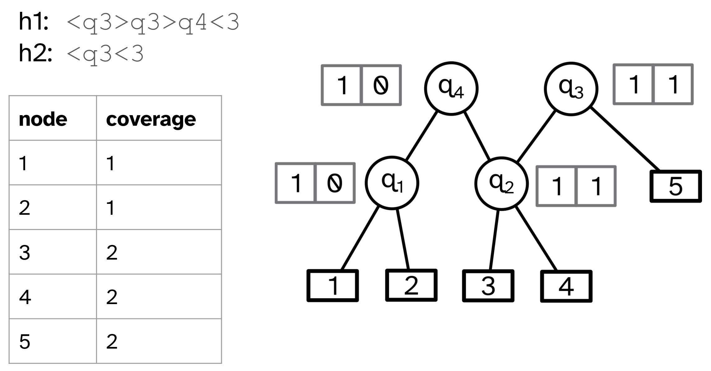
Table is constructed in a bottom-up traversal of the directed acyclic graph constituting the grammar. In each step, one of the following two cases applies to the currently processed meta-node :
-
1.
Meta-node is already an anchoring meta-node, and therefore, its left-most and right-most anchoring meta-node is itself. Accordingly, is stored in with size , corresponding to the number of its children, and offsets .
-
2.
Otherwise, we determine ’s size, its left-most and right-most anchoring meta-node, and their offsets by looking up ’s children in .
We then construct table by iterating over all top-level meta-nodes, and creating for each such meta-node entries in that map digram occurrences associated with its left-most and right-most anchoring meta-node to itself.
Runtime.
In the following, we study the runtime of our algorithm under a grammar where each production rule maps to exactly two (meta-)nodes, as it is the case prior to rule reduction. This will simplify the analysis, which operates on the directed acyclic graph structure underlying the grammar, but does not change its outcome: If we remove a meta-node , then all the edges to ’s children are moved to ’s parent. Additionally, the edge between and its parent is removed. The total numbers of edges and nodes are reduced by one, respectively. Therefore, we can analyze without loss of generality the grammar before reduction, as it becomes only smaller through the reduction process.
Since we know the sizes of and in advance, we can pre-allocate the exact amount of memory, allowing us time insertions. The construction of has to iterate over all the meta-nodes of the grammar. The lookup of the children of each meta-node is performed in constant time by querying . Thus, the runtime of ’s construction is limited by .
To construct , again all the rules are iterated, however this time also all of its digram occurrences are traversed. If the meta-nodes are processed in top-down order, we can simply create a hash set of all the digram occurrences whose top-level meta-nodes were already visited. Then the check whether a node is a top-level node can be done in time. Since all of the remaining instructions are also constant-time look-ups, the runtime is bounded by the number of total digram occurrences, which is .
Haplotype encoding is performed by iterating over all digram occurrences. Inside the loop, each iteration adds at most one element to the stack. This means we can pop only as much elements as we have iterations. Additionally, the final stack for each haplotype has at most the length of the inner loop, meaning the print instruction has the same complexity as the inner loop. Therefore the whole runtime is depending only on the number of digram occurrences, limiting the worst-case runtime to .
2.7 Coverage computation with compressed haplotypes
In this section, we provide evidence that the compressed grammar can serve as an efficient in-memory data structure and speed up haplotype analysis while simultaneously reducing memory usage. To this end, we address the task of computing a node coverage table. In this table each vertex of the pangenome graph is recorded with the number of haplotypes in which it appears at least once.
For this task, the grammar-encoded haplotype paths do not need to be decompressed. In fact, the calculation can be even more efficient by exploiting the directed acyclic graph that underlies the grammar. We iterate over the encoded haplotypes and produce presence/absence lists for all the (meta-)nodes, similar to how this process is done on uncompressed haplotypes. However, since the compressed haplotypes are shorter than uncompressed counterparts this process is faster. In the next step, the presence/absence lists are pushed down the directed acyclic graph using a top-down approach, as seen in Figure 4(b). Lists from parental meta-nodes are combined using disjunction. Thereafter, lists of the leaf nodes are collected and summed to produce the reported coverage table.
3 Results
We implemented our method, sqz, in Rust and released the source code under the MIT license at https://github.com/codialab/sqz.
We evaluated sqz on three human pangenome graphs:
The full version of the HPRC v2.0 MC GRCh38 graph includes complete assemblies, but alignment quality is poor in certain regions. Particularly centromeres contain essentially large chunks of unaligned sequence. In contrast, the clipped version removes these segments, limiting the pangenome graph to regions with reliable alignments.
We benchmarked our method against three compression tools: bgzip [1], gbz [23], and sequitur [15]. bgzip produces gzip-compatible compressed binary files and is widely used for compressing pangenome graphs in the GFA format, primarily because its output can be decompressed with gzip, which is pre-installed on most Unix systems. Its key advantage over gzip is support for indexing, allowing selective decompression of file segments. gbz, in contrast, is specifically designed for compressing pangenome graphs and integrates with tools in the GBWT ecosystem, as discussed in Section 1. sequitur is a classical grammar-based compression algorithm in natural language processing (NLP).
Among existing BPE based algorithms, Re-Pair [13] is most similar to our approach. Both algorithms iteratively replace the most frequent digram with a production rule or meta-node, proceeding in descending order of frequency. However, Re-Pair operates on linear text rather than graph structures, and it does not account for inverted digrams, unlike sqz and gbz. Although several Re-Pair implementations are available, many operate solely on text or binary files and are not designed to handle characters spanning multiple bytes. Therefore, we were unable to successfully apply them to haplotype paths, which are composed of node identifiers that cannot be represented by a single byte.
In contrast, we were able to evaluate sequitur [15], another BPE algorithm. sequitur constructs and applies production rules as soon as it reads a repeated digram. As a result, sequitur’s memory usage scales with the size of the compressed output rather than the input. However, its compression performance depends on the input order, since it processes digrams in the order they appear rather than by frequency. sequitur allows the user to set the size of its core data structure, a hash table. This affects both memory usage and runtime: larger tables reduce collisions and improve performance at the cost of increased memory. For all evaluations, we set the hash table size to 2,000 MB, which was the maximum value supported by the program.
As an initial experiment, we used the Chr19 pangenome to evaluate how compression scales with the number of haplotypes in a pangenome graph. To this end, we randomly removed haplotypes until only a specified number remained, and removed all S- and L-lines corresponding to nodes and edges that are not covered by the remaining subset. We then applied sqz, bgzip, sequitur, and gbz to the resulting trimmed graphs. Additionally, we tested a combined approach using sqz followed by bgzip compression, as bgzip is commonly used in transferring GFA files. The same thing we also did for gbz.
The resulting file sizes and compression ratios are shown in Figure 5. The compression ratio is defined as . bgzip exhibits constant compression behavior: file size increases linearly with the number of haplotypes, and the compression ratio remains constant at about a rate of . For fewer than 100 haplotypes, bgzip achieves better compression than the purely grammar-based approaches sqz and sequitur. For all other methods, the compression ratio improves as more haplotypes are added, benefiting from increased redundancy. Up to 100 haplotypes, the difference between sqz and sequitur remains small (e.g., GB vs. GB), but it gets larger with increasing number of haplotypes. Among all methods, gbz+bgzip delivers the best compression results. sqz+bgzip slightly outperforms gbz for fewer haplotypes.
A second benchmark was conducted on the clipped and full HPRC v2.0 MC GRCh38 graphs, that have been split up into their individual chromosome graphs. This setup enables an evaluation of how compression performance is affected by the similarity among haplotypes, due to the full graphs containing less similar haplotype paths than their clipped counterparts.
Due to the large input sizes (up to 36 GB), we were unable to run sequitur for this benchmark, as it required excessive runtimes. We evaluated compression performance in terms of both file size and compression ratio. For the clipped graphs, sqz+bgzip and gbz perform similarly again, achieving compression ratios between 60 and 80, depending on the specific graph. sqz alone achieves a compression ratio of around 20, while bgzip performs worst overall. The best result achieves gbz+bgzip, reaching compression ratios of up to 150. Except for bgzip, compression results on the full graphs vary considerably, as the amount of heterochromatic sequence differs across chromosomes. For chromosomes 1 through 11, bgzip typically outperforms sqz, but from chromosome 12 onward, sqz yields smaller files, with the exception of chromosomes 1 and 9. gbz consistently produces smaller files than bgzip, while the combined gbz+bgzip approach generally results in the smallest file sizes. With the exception of chromosome 9, sqz+bgzip is always very close in terms of resulting file size.
To assess how effectively haplotypes are compressed using sqz, we examined the number of nodes per haplotype for each chromosome in the clipped graphs, illustrated in Figure 7. sqz achieves a reduction in haplotype length by more than two orders of magnitude. This analysis also reveals a non-negligible variance across haplotypes, with some chromosomes, e.g., chromosome 15, containing haplotypes that are much less compressed than others.
Another key consideration when working with large files is the runtime and memory consumption of the compression algorithm. We compared the performance of sequitur, sqz, gbz and bgzip on the Chr19 pangenome using the set of trimmed graphs containing a varying numbers of haplotypes that we constructed for the first experiment.
In terms of runtime, sequitur outperforms sqz on graphs with up to 800 haplotypes. However, for the two largest graphs with 900 and 1,000 haplotypes, sqz is faster and, for the latter graph, requires more than an hour less runtime. The fastest method, however, is gbz (with the exception of the smallest two graphs, where bgzip is equally as fast or faster). On memory usage, bgzip performs the best by having a constantly very low memory usage. Still, sequitur and gbz outperform sqz by a wide margin. Even for the largest graph, sequitur stays below 5 GB of memory usage and gbz below 20 GB, while sqz requires up to 176 GB.
To evaluate the performance of computing coverage tables using the in-memory representation of the grammar, we implemented two Python scripts that make use of libraries networkx and numpy. One does the calculation on an uncompressed GFA file of the Chr19 pangenome. The second one follows the approach described in the previous section and takes a GFA file compressed by sqz. The script for the uncompressed GFA file takes 7:49 min, while the one on the sqz-compressed graph only takes 2:39 min. The memory usage is reduced over ten-fold when using the script with the compressed graph, requiring only 14.8 GB instead of 159.6 GB. We also ran the two approaches over all of the HPRC v2.0 graphs (clipped and full), the results are shown in Figure 8. Similar to the Chr19 graph, working with the grammar-based strategy is faster and uses less memory for all chromosomes. Particularly, the difference in terms of runtime is large, with the original method needing 2:08 hrs, while the compressed files only need 12 min for the clipped chromosome 1.
| Haplo-types | time (min) | memory (GB) | ||||||
|---|---|---|---|---|---|---|---|---|
| sequitur | sqz | gbz | bgzip | sequitur | sqz | gbz | bgzip | |
| 100 | 6 | 11 | 2 | 1 | 2.3 | 16.3 | 1.8 | 0.01 |
| 200 | 13 | 26 | 4 | 4 | 2.7 | 30.1 | 3.7 | 0.01 |
| 300 | 23 | 45 | 6 | 7 | 2.9 | 50.2 | 5.2 | 0.01 |
| 400 | 31 | 60 | 8 | 10 | 3.3 | 57.4 | 6.7 | 0.01 |
| 500 | 45 | 84 | 10 | 14 | 3.5 | 89.4 | 9.7 | 0.01 |
| 600 | 58 | 91 | 12 | 17 | 3.7 | 96.0 | 11.2 | 0.01 |
| 700 | 84 | 107 | 14 | 21 | 4.0 | 103.2 | 12.7 | 0.01 |
| 800 | 108 | 124 | 16 | 24 | 4.1 | 110.2 | 14.1 | 0.01 |
| 900 | 169 | 152 | 18 | 31 | 4.4 | 154.3 | 15.6 | 0.01 |
| 1000 | 289 | 223 | 20 | 34 | 4.7 | 175.8 | 17.0 | 0.01 |
4 Discussion and Outlook
By introducing Q- and Z-records, we propose an extension to the GFA format that supports human-readable, grammar-based compression. Grammar-based compression is simple and intuitive, yet is as effective as any finite-state compression scheme [10]. It is highly versatile and has given rise to a broad body of research, resulting in a variety of compression schemes [9]. Our proposed GFA extension fully supports incremental updates: nodes and edges can be added to the graph without interfering with the grammar captured in Q-records. Likewise, new haplotypes can be encoded using the existing grammar, although this may lead to less efficient compression. In addition, common pangenome graph modifications, such as “unchopping”, i.e., the merging of a universal digram into a single node or the decomposition of a node into a series of smaller ones, affect the grammar only locally such that at most a few low-level meta-nodes need to be updated. Most importantly, we argue that grammar-encoded haplotypes need not be decompressed for analysis. Instead, they enable faster and more memory-efficient haplotype analysis, without the need to use dedicated external libraries. The simplicity of the grammar allows it to be represented by data structures available in widely used scripting languages such as Python.
Our BPE-based implementation, sqz, serves as a proof of concept for the proposed GFA extension. sqz often achieves higher compression ratios than bgzip and sequitur, and performs on par with gbz when combined with bgzip. The latter combination is only outperformed by gbz+bgzip that provides an even higher compression ratio. However, sqz offers an advantage over gbz in that it provides a simple, human-readable, and easily modifiable encoding.
We envision further variants of grammar based encodings that can be realized with our proposed GFA extension, such as grammars based on -grams for , or grammars derived from maximal exact matches (MEMs) which are widely used in pangenomics [20]. Moreover, Q-records can carry biological meaning by annotating shared sequences associated with specific alleles. This enables not only compression, but also allows to encode haplotypes as combinations of alleles, embodying a natural, biologically motivated representation.
Conceptually, our proposal represents a dichotomy to existing approaches in pangenomics that encode differences between haplotypes, such as snarl decomposition [17, 2] or reference-based variant formats like the variant call format (VCF). We argue that capturing commonalities rather than differences offers several advantages. First, decompression does not require an external reference or computationally intensive edit operations to reconstruct the original sequence. Second, there is often no unique or universally accepted way to represent differences, leading to arbitrary decisions that impede comparability across datasets, a challenge exemplified by the persistent difficulties in VCF merging [11, 4]. Nevertheless, some of these representations could potentially be reconciled with our grammar-based approach. For example, a snarl decomposition can naturally give rise to a simple grammar, where each tip and each shared block within a chain, as well as each distinct variant within a snarl, is represented as a meta-node.
References
- [1] James K. Bonfield, John Marshall, Petr Danecek, Heng Li, Valeriu Ohan, Andrew Whitwham, Thomas Keane, and Robert M. Davies. HTSlib: C library for reading/writing high-throughput sequencing data. GigaScience, 10(2):giab007, 2021. doi:10.1093/gigascience/giab007.
- [2] Xian Chang, Jordan Eizenga, Adam M Novak, Jouni Sirén, and Benedict Paten. Distance indexing and seed clustering in sequence graphs. Bioinformatics, 36(Suppl_1):i146–i153, July 2020. doi:10.1093/bioinformatics/btaa446.
- [3] Jana Ebler, Peter Ebert, Wayne E Clarke, Tobias Rausch, Peter A Audano, Torsten Houwaart, Yafei Mao, Jan O Korbel, Evan E Eichler, Michael C Zody, Alexander T Dilthey, and Tobias Marschall. Pangenome-based genome inference allows efficient and accurate genotyping across a wide spectrum of variant classes. Nat. Genet., 54:518–525, 2022. doi:10.1038/s41588-022-01043-w.
- [4] Adam C English, Vipin K Menon, Richard A Gibbs, Ginger A Metcalf, and Fritz J Sedlazeck. Truvari: refined structural variant comparison preserves allelic diversity. Genome Biol., 23(1):271, December 2022. doi:10.1186/s13059-022-02840-6.
- [5] Yang Gao, Xiaofei Yang, Hao Chen, Xinjiang Tan, Zhaoqing Yang, Lian Deng, Baonan Wang, Shuang Kong, Songyang Li, Yuhang Cui, Chang Lei, Yimin Wang, Yuwen Pan, Sen Ma, Hao Sun, Xiaohan Zhao, Yingbing Shi, Ziyi Yang, Dongdong Wu, Shaoyuan Wu, Xingming Zhao, Binyin Shi, Li Jin, Zhibin Hu, Chinese Pangenome Consortium (CPC), Yan Lu, Jiayou Chu, Kai Ye, and Shuhua Xu. A pangenome reference of 36 chinese populations. Nature, 619:112–121, 2023. doi:10.1038/s41586-023-06173-7.
- [6] Cristian Groza, Carl Schwendinger-Schreck, Warren A Cheung, Emily G Farrow, Isabelle Thiffault, Juniper Lake, William B Rizzo, Gilad Evrony, Tom Curran, Guillaume Bourque, and Tomi Pastinen. Pangenome graphs improve the analysis of structural variants in rare genetic diseases. Nat. Commun., 15:657, 2024. doi:10.1038/s41467-024-44980-2.
- [7] Peter Heringer and Daniel Doerr. sqz. Software, swhId: swh:1:dir:d7c4cb1cc536abc10166918dda34b0b373987c7b (visited on 2025-08-04). URL: https://github.com/codialab/sqz, doi:10.4230/artifacts.24320.
- [8] Simon Heumos, Michael L Heuer, Friederike Hanssen, Lukas Heumos, Andrea Guarracino, Peter Heringer, Philipp Ehmele, Pjotr Prins, Erik Garrison, and Sven Nahnsen. Cluster-efficient pangenome graph construction with nf-core/pangenome. Bioinformatics, 40:btae609, 2024. doi:10.1093/bioinformatics/btae609.
- [9] J Kieffer and E Yang. Survey of grammar-based data structure compression. IEEE BIT Inf Theory Mag, 2:19–35, 2022. doi:10.1109/MBITS.2022.3210891.
- [10] J C Kieffer and En-Hui Yang. Grammar-based codes: a new class of universal lossless source codes. IEEE Trans. Inf. Theory, 46(3):737–754, May 2000. doi:10.1109/18.841160.
- [11] Melanie Kirsche, Gautam Prabhu, Rachel Sherman, Bohan Ni, Alexis Battle, Sergey Aganezov, and Michael C Schatz. Jasmine and iris: population-scale structural variant comparison and analysis. Nat. Methods, 20(3):408–417, March 2023. doi:10.1038/s41592-022-01753-3.
- [12] Taku Kudo and John Richardson. SentencePiece: A simple and language independent subword tokenizer and detokenizer for neural text processing. arXiv [cs.CL], 2018. arXiv:1808.06226.
- [13] N.J. Larsson and A. Moffat. Off-line dictionary-based compression. Proceedings of the IEEE, 88(11):1722–1732, 2000. doi:10.1109/5.892708.
- [14] Wen-Wei Liao, Mobin Asri, Jana Ebler, Daniel Doerr, Marina Haukness, Glenn Hickey, Shuangjia Lu, Julian K Lucas, Jean Monlong, Haley J Abel, Silvia Buonaiuto, Xian H Chang, Haoyu Cheng, Justin Chu, Vincenza Colonna, Jordan M Eizenga, Xiaowen Feng, Christian Fischer, Robert S Fulton, Shilpa Garg, Cristian Groza, Andrea Guarracino, William T Harvey, Simon Heumos, Kerstin Howe, Miten Jain, Tsung-Yu Lu, Charles Markello, Fergal J Martin, Matthew W Mitchell, Katherine M Munson, Moses Njagi Mwaniki, Adam M Novak, Hugh E Olsen, Trevor Pesout, David Porubsky, Pjotr Prins, Jonas A Sibbesen, Jouni Sirén, Chad Tomlinson, Flavia Villani, Mitchell R Vollger, Lucinda L Antonacci-Fulton, Gunjan Baid, Carl A Baker, Anastasiya Belyaeva, Konstantinos Billis, Andrew Carroll, Pi-Chuan Chang, Sarah Cody, Daniel E Cook, Robert M Cook-Deegan, Omar E Cornejo, Mark Diekhans, Peter Ebert, Susan Fairley, Olivier Fedrigo, Adam L Felsenfeld, Giulio Formenti, Adam Frankish, Yan Gao, Nanibaa’ A Garrison, Carlos Garcia Giron, Richard E Green, Leanne Haggerty, Kendra Hoekzema, Thibaut Hourlier, Hanlee P Ji, Eimear E Kenny, Barbara A Koenig, Alexey Kolesnikov, Jan O Korbel, Jennifer Kordosky, Sergey Koren, Hojoon Lee, Alexandra P Lewis, Hugo Magalhães, Santiago Marco-Sola, Pierre Marijon, Ann McCartney, Jennifer McDaniel, Jacquelyn Mountcastle, Maria Nattestad, Sergey Nurk, Nathan D Olson, Alice B Popejoy, Daniela Puiu, Mikko Rautiainen, Allison A Regier, Arang Rhie, Samuel Sacco, Ashley D Sanders, Valerie A Schneider, Baergen I Schultz, Kishwar Shafin, Michael W Smith, Heidi J Sofia, Ahmad N Abou Tayoun, Françoise Thibaud-Nissen, Francesca Floriana Tricomi, Justin Wagner, Brian Walenz, Jonathan M D Wood, Aleksey V Zimin, Guillaume Bourque, Mark J P Chaisson, Paul Flicek, Adam M Phillippy, Justin M Zook, Evan E Eichler, David Haussler, Ting Wang, Erich D Jarvis, Karen H Miga, Erik Garrison, Tobias Marschall, Ira M Hall, Heng Li, and Benedict Paten. A draft human pangenome reference. Nature, 617:312–324, 2023. doi:10.1038/s41586-023-05896-x.
- [15] C Nevill-Manning and I Witten. Identifying hierarchical structure in sequences: A linear-time algorithm. J. Artif. Intell. Res., 7:67–82, 1997. doi:10.1613/JAIR.374.
- [16] Luca Parmigiani, Erik Garrison, Jens Stoye, Tobias Marschall, and Daniel Doerr. Panacus: fast and exact pangenome growth and core size estimation. Bioinformatics, 40:2024.06. 11.598418, 2024. doi:10.1101/2024.06.11.598418.
- [17] Benedict Paten, Jordan M Eizenga, Yohei M Rosen, Adam M Novak, Erik Garrison, and Glenn Hickey. Superbubbles, ultrabubbles, and cacti. J. Comput. Biol., 25(7):649–663, July 2018. doi:10.1089/cmb.2017.0251.
- [18] Ivan Provilkov, Dmitrii Emelianenko, and Elena Voita. BPE-dropout: Simple and effective subword regularization. arXiv [cs.CL], 2019. arXiv:1910.13267.
- [19] Rico Sennrich, Barry Haddow, and Alexandra Birch. Neural machine translation of rare words with subword units. In Katrin Erk and Noah A Smith, editors, Proceedings of the 54th Annual Meeting of the Association for Computational Linguistics (Volume 1: Long Papers), pages 1715–1725. Association for Computational Linguistics, 2016. doi:10.18653/v1/P16-1162.
- [20] Vikram S. Shivakumar and Ben Langmead. Mumemto: efficient maximal matching across pangenomes. bioRxiv, 2025. doi:10.1101/2025.01.05.631388.
- [21] Jonas A Sibbesen, Jordan M Eizenga, Adam M Novak, Jouni Sirén, Xian Chang, Erik Garrison, and Benedict Paten. Haplotype-aware pantranscriptome analyses using spliced pangenome graphs. Nat. Methods, 20:239–247, 2023. doi:10.1038/s41592-022-01731-9.
- [22] Jouni Sirén, Jean Monlong, Xian Chang, Adam M Novak, Jordan M Eizenga, Charles Markello, Jonas A Sibbesen, Glenn Hickey, Pi-Chuan Chang, Andrew Carroll, Namrata Gupta, Stacey Gabriel, Thomas W Blackwell, Aakrosh Ratan, Kent D Taylor, Stephen S Rich, Jerome I Rotter, David Haussler, Erik Garrison, and Benedict Paten. Pangenomics enables genotyping of known structural variants in 5202 diverse genomes. Science, 374:abg8871, 2021. doi:10.1126/science.abg8871.
- [23] Jouni Sirén and Benedict Paten. GBZ file format for pangenome graphs. Bioinformatics, 38(22):5012–5018, 2022. doi:10.1093/bioinformatics/btac656.
- [24] Hervé Tettelin, David Riley, Ciro Cattuto, and Duccio Medini. Comparative genomics: the bacterial pan-genome. Curr. Opin. Microbiol., 11:472–477, 2008. doi:10.1016/j.mib.2008.09.006.