Sequence Similarity Estimation by Random Subsequence Sketching

Abstract
Sequence similarity estimation is essential for many bioinformatics tasks, including functional annotation, phylogenetic analysis, and overlap graph construction. Alignment-free methods aim to solve large-scale sequence similarity estimation by mapping sequences to more easily comparable features that can approximate edit distances efficiently. Substrings or -mers, as the dominant choice of features, face an unavoidable compromise between sensitivity and specificity when selecting the proper -value. Recently, subsequence-based features have shown improved performance, but they are computationally demanding, and determining the ideal subsequence length remains an intricate art. In this work, we introduce SubseqSketch, a novel alignment-free scheme that maps a sequence to an integer vector, where the entries correspond to dynamic, rather than fixed, lengths of random subsequences. The cosine similarity between these vectors exhibits a strong correlation with the edit similarity between the original sequences. Through experiments on benchmark datasets, we demonstrate that SubseqSketch is both efficient and effective across various alignment-free tasks, including nearest neighbor search and phylogenetic clustering. A C++ implementation of SubseqSketch is openly available at https://github.com/Shao-Group/SubseqSketch.
Keywords and phrases:
Alignment-free sequence comparison, Phylogenetic clustering, Nearest neighbor search, Edit distance embeddingCopyright and License:
2012 ACM Subject Classification:
Applied computing Bioinformatics ; Applied computing Computational biologySupplementary Material:
Software (Source Code): https://github.com/Shao-Group/SubseqSketcharchived at
Funding:
This work is supported by the US National Science Foundation (DBI-2019797 to M.S.) and the US National Institutes of Health (R01HG011065 to M.S.).Editors:
Broňa Brejová and Rob PatroSeries and Publisher:
1 Introduction
Estimating the similarity between biological sequences is a fundamental task in bioinformatics, underpinning a wide range of applications including homology detection, gene annotation, and phylogenetic analysis. Traditionally, sequence similarity has been assessed with alignment-based methods, which attempt to find an optimal correspondence between characters from two or more sequences. While providing the most accurate results, these methods often suffer from high computational cost, especially when applied to large and divergent datasets.
Sketching-based methods have been developed to address this limitation. A sketch summarizes a long sequence into a small set of representative fingerprints that can be rapidly compared in place of the original sequences for similarity estimation. Together with its variants, the most widely used sketching method is MinHash (MH) [2]. In its simplest form, MH utilizes a hash function that maps each -mer of a sequence to a number and only keeps the -mer with the minimum hash value as the representative of that sequence. It is easy to see that the probability for two sequences to be represented by the same -mer is proportional to the Jaccard similarity of the two sequences (viewed as sets of -mers), namely, the number of shared -mers between the sequences normalized by the total number of distinct -mers among them. Hence, by repeatedly choosing min--mers with different hash functions and keeping track of the number of occurrences that the picked -mers match between the two sequences, the Jaccard similarity can be estimated. In this process, the list of all representative -mers of a sequence is called the MH sketch of this sequence. Two MH sketches are compared by the Hamming similarity – number of identical -mers at the same indices. Order Min Hash (OMH) [20] extends this idea by estimating the weighted Jaccard similarity. Instead of picking one representative -mer at a time, each entry of an OMH sketch is generated by picking several -mers and putting them together following the original order in the sequence. OMH has been proved to be a locality-sensitive hashing family for the edit distance. A more comprehensive review of sketching algorithms for genomic data can be found in [22]. Note that both MH and OMH can be considered substring-based sketching methods because they pick substrings as the representatives. They therefore face the commonly observed difficulty in choosing a proper : larger is desirable to eliminate spurious matches but there are very few shared long -mers even between closely related sequences.
To address this fundamental limitation of -mers, several recent works [15, 12, 14] have advocated for the use of unrestricted subsequences instead. Subsequences relax the requirement that matching base pairs must be consecutive, allowing them to naturally tolerate gaps in the underlying – often unknown and computationally expensive – true alignment between sequences. This enables the identification of longer and hence more reliable matches, which in turn enhances the accuracy of downstream tasks. To fully leverage the benefits of subsequences, one must overcome a key algorithmic challenge: unlike the linear number of -mers in a sequence, the number of subsequences grows exponentially, making MH-like strategies that rely on enumerating all candidates impractical. In this work, we seek to exploit structural properties of subsequences to overcome this computational barrier. To this end, we develop SubseqSketch, an efficient sketching method that summarizes long sequences into compact, subsequence-based features that are highly correlated with edit similarities. Through experiments on typical downstream applications, including nearest neighbor search and phylogenetic clustering, we demonstrate that SubseqSketch is both efficient and effective.
1.1 Related work
Recently, a sketching method named LexicHash [9] proposes to compare sketches based on the length of their common prefixes, rather than relying on fully matched -mers. This has the effect of sketching with -mers for all lengths up to a predefined maximum value. However, LexicHash still suffers from the common issue of -mer-based methods, namely, a small number of edits can destroy all long -mer matches between two similar sequences. Furthermore, LexicHash is designed for the task of overlap detection, rather than estimating the similarity between two sequences. In particular, the authors define the LexicHash similarity score between two sequences as the length of the longest matching prefix among their sketches. Hence, a score only indicates that the two sequences share a common -mer, which may be effective for detecting overlapping reads, but appears to be insufficient for edit similarity estimation (see Figure 4). In their follow-up work LexicMap [26], the authors design a sequence alignment tool that uses the identified common -mers as seeds, effectively employing LexicHash as a seeding method rather than a sketching method. See Section 4 for further discussion of the differences between sketching and seeding.
To the best of our knowledge, the only existing subsequence-based sketching method is Tensor Slide Sketch (TSS) [12]. Instead of picking -mers from the input sequence, TSS aims at producing a sketch by counting the occurrences of all subsequences. Since there is an exponential number of them, TSS has to group subsequences in a smart way to facilitate counting. However, to make it efficient, TSS is restricted to count all short subsequences, which limits its capacity in distinguishing similar and dissimilar sequences.
A closely related line of research focuses on embedding edit distance into metric spaces. Most notably, the CGK embedding [4] maps sequences into Hamming space with bounded distortion and, when combined with locality-sensitive hashing techniques, has been applied to various bioinformatics tasks, including edit similarity joins [29] and overlap detection [27]. However, CGK maps a sequence of length to one of length , making it unsuitable as an efficient sketching method, where the goal is to reduce representation size. To take advantage of the structure of the underlying data, machine learning methods have been developed that learn embeddings outperforming CGK in downstream applications [5], despite lacking its theoretical guarantees. These approaches, however, require training data with known edit distances, limiting their applicability to tasks involving long sequences, such as genome phylogeny.
2 SubseqSketch
The idea of SubseqSketch is to identify long common subsequences between input sequences through random sampling. Computing the sketch of a sequence can be figuratively thought of as answering a survey in which each question asks whether contains a randomly selected sequence as a subsequence. By comparing the answers of two sequences, their similarity can be estimated. For a concrete example, according to Figure 3, if length- sequences (over the DNA alphabet ) are taking our survey, we can choose a query sequence to have length and expect half of the answers to be “yes”. Furthermore, a matching “yes” answer for a pair of sequences suggests a (partial) alignment between them that involves at least a quarter of their bases. We note that this idea does not work well with substrings (-mers): As the number of -mers in a sequence is negligible compared to the number of length- subsequences, the chance of successfully finding a reasonably sized common substring by random sampling is low, even between highly similar sequences. Continuing the previous example, if we were to ask whether an -mer is a substring, the vast majority of sequences would respond “no”; on the other hand, querying with - or -mers yields more balanced responses, but a matching “yes” answer carries little information due to the short length of the common substring. In both cases, we can only expect to get a very weak, if functional at all, classifier for distinguishing between similar and dissimilar sequences.
While sampling long subsequences is beneficial for similarity estimation, it becomes computationally expensive on long inputs. In the following section, we introduce the concept of tokenization to effectively generalize the above strategy to genome-scale sequences. Combined with the idea of an “enhanced survey”, where binary yes/no questions are upgraded to integer-scale queries, we present the full-fledged SubseqSketch as an effective and efficient sketching method.
2.1 Tokenized subsequence
A sequence of length over an alphabet can be viewed as a sequence of “tokens” each of which is a string of length . We say is a tokenized subsequence of a length- sequence if there is a list of indices such that the length- substring of starting at matches the -th token of . Note that when , a tokenized subsequence is a regular subsequence; it is not necessarily the case when , as the tokens are allowed to overlap, see Figure 1 for an example.
2.2 Construction of SubseqSketch
To construct SubseqSketch for input sequences, we first generate a list of random sequences of length each, where and are predefined parameters. We call the list of testing sequences. Two SubseqSketches are comparable only if they were generated with the same list ; in this sense, serves as shared randomness in the sketching process, analogous to the shared random ordering of -mers in MH sketches. Given an input sequence and a testing sequence in , SubseqSketch determines the maximum number of prefix tokens in that form a tokenized subsequence of . The resulting vector consists of integers, one for each testing sequence. This vector is the sketch of , denoted as . See Figure 2 for an illustration.
A straightforward linear scan computes the sketch entries in time. This worst-case time complexity can be improved by preprocessing the input sequence to build an index that facilitates rapid lookup for the occurrence of the next token of a testing sequence. For example, for token size , we can build an automaton on in time and space. In the automaton, each character stores pointers. The pointer corresponding to points to the next appearance of after (or null if no exists after ). Then for a testing sequence , we can simply follow the pointers according to the characters of , until either a null pointer is encountered or is exhausted. This takes time for each testing sequence so the total sketching time is .
For larger token size, a similar idea can be applied: we can preprocess to build a lookup table of size where each entry records the occurring positions of that token on , either in a sorted array or some other data structures that supports quick search. Each testing sequence can then be processed by following this lookup table until all tokens are used or the end of a position array is reached. This allows each integer in the sketch to be computed in time, instead of a linear search. We provide this preprocessing approach as an option in our implementation. However, through experiments we found that the linear search std::string::find provided in the standard C++ library is almost always faster. The overhead of preprocessing may only be justified for a large number of very long testing sequences with a small token size, which is not a recommended setting for our sketching algorithm (see Section 2.4).
2.3 Choice of similarity function
The SubseqSketch of a sequence provides a highly informative representation of . To build intuition, consider two sequences and . If both sketches show large numbers at the same index, then and must share a long tokenized subsequence and are hence likely similar in terms of the edit distance. Conversely, if one sketch has a large value while the other has a small value at the same index, it suggests that the sequences are likely dissimilar.
As with other sketching methods, a similarity measure over the sketches is required to translate the above intuition into a quantitative score that accurately reflects the true similarity between input sequences. Methods that compare sketches for equality at corresponding indices, such as MH and OMH, naturally employ Hamming similarity, which counts the number of matching entries between sketches. SubseqSketch, on the other hand, generates integer-valued vectors, enabling the use of a wide range of well-established distance/similarity metrics. We empirically evaluate a list of metrics using the data from Section 3.1. SubseqSketches are first computed, after which similarity scores are calculated using various metrics. The Pearson correlations between these scores and the ground truth edit similarities are reported in Table 1.
| Metric | Pearson correlation |
|---|---|
| Canberra | |
| Bray-Curtis | |
| Correlation | |
| Cosine | |
| Hamming | |
| Manhattan | |
| Squared Euclidean | |
| Jaccard | |
| Euclidean | |
| Minkowski | |
| Chebyshev |
As shown in the table, cosine similarity is among the most effective metrics for producing estimates that are strongly correlated with the true edit similarity. According to its definition,
where denotes the vector dot product, pairwise cosine similarities between two sketching matrices can be computed using a single matrix multiplication (assuming the rows are normalized), which is highly optimized in modern hardware and numerical libraries. We therefore adopt cosine similarity between SubseqSketches in our implementation for its effectiveness and computational efficiency.
2.4 Choice of parameters
SubseqSketch has three parameters: the token size , the number of tokens in each testing sequence, and the size of the testing list. The parameter controls the size of the sketches. In particular, a SubseqSketch takes bits space to store. As with other sketching methods, increasing the sketch size improves estimation accuracy but comes at the cost of greater time and storage requirements. In the experimental sections, we compare the sketching methods at the same sketch size.
The parameters and are related. In the resulting sketches, each entry is an integer between and . If is too large (for example, close to the input length ), most entries would be ; on the other hand, if both and are small, most entries would reach the maximum possible value at , regardless of the input sequence . Neither case is desirable as the sketches cannot provide a strong distinction between similar and dissimilar input sequences. Note that we can always choose a large to ensure that few, if any, sketch entries reach the maximum value. However, this increases the sketch file size, as each entry requires bits – an inefficient use of space if most entries are significantly smaller than .
We now try to derive an optimal choice of for . In a recent paper [8], the authors motivated their sequence sampling method with an interesting puzzle (paraphrased): is the number of DNA 5-mers containing the substring ACGT the same as that for the substring AAAA? Astute readers will immediately answer “no” because it is impossible for a 5-mer to both start and end with ACGT – taking the union of the two disjoint groups gives the correct number – which is not the case for AAAA whose symmetry would cause the same strategy to double-count the 5-mer AAAAA.
As a curious extension, the same question can be asked, replacing substring with subsequence, namely, we do not require the containment to be consecutive. This seemingly more complicated version turns out to have a counterintuitively nicer answer: the number of -mers containing a given -mer as a subsequence is a function of and , independent of the choice of the -mer. Consider a length- sequence , we count the number of length- sequences whose subsequence is . To avoid over-counting, we only count if is the first occurrence of in . It means the characters in before cannot be , leaving them choices each. The same holds for regions in between and , and finally all characters after are free to be anything in . This leads to choices. Note that the expression only depends on (i.e., any combination of yields the same number), so we can group the terms and sum over choices of to get the answer
We emphasize that the above calculation is independent of the chosen sequence . An example is shown in Figure 3.
Given the length of the input sequences, we can use this formula to find a such that at most a small threshold fraction (e.g., ) of the sketch entries reach the maximum value . For the example in Figure 3 where , would suffice.
For larger , the derivation is not as neat. We can view a regular sequence over the alphabet as a tokenized sequence over the alphabet and apply the above formula. But unlike adjacent characters in the original sequence, consecutive tokens with an overlap of length are not independent, causing the formula to significantly overestimate. Since using a small makes the sketching faster to compute and smaller to store, with an exception in Table 3, we fix in the following experiments (namely, each entry in the sketch fits in 4 bits) and aim to choose to ensure the sketching entries are neither too small nor maxed out. Table 2 provides empirical recommendations for across common input sizes .
2.5 Sample subsequences from input
Using randomly generated testing sequences is the best one can do in a data-oblivious setting, while better performance can usually be achieved if we can afford to adjust the sketches according to the input data. One idea to introduce data dependency is to sample subsequences from the input to form the testing list. This is particularly suitable when the input comprises a small number of sequences – for example, when estimating phylogenetic distances among a group of closely related genomes, as shown in Section 3.3. On the other hand, if the sketches are used to build an index of a large database of sequences to handle queries, it may not be practical to re-sketch the entire database with a new testing list for each query. In this situation, we simply use the data-oblivious version with a fixed list of randomly generated testing sequences and demonstrate in Sections 3.1 and 3.2 that it already achieves good performance.
3 Experiments
In this section, we first show a strong correlation between the cosine similarity of SubseqSketches with the edit similarity between simulated pairs of sequences. Then the sketch quality of SubseqSketch is tested on two sequence comparison tasks, the nearest neighbor search and phylogeny reconstruction. In each task, we compare SubseqSketch with competing methods on both simulated sequences and published benchmark datasets. For a fair comparison, each method is set to produce sketches of (roughly) the same size. A grid search is performed for each competing method to find the best parameters. Details are reported in each subsection.
3.1 Correlation between sketch similarity and edit similarity
To directly compare the sketch similarity against the desired but much more expensive to compute edit similarity, we generate random DNA sequences of length . Each sequence is randomly mutated (an insertion, deletion, or substitution) for a random number of rounds up to to produce a pairing sequence. For each pair, we compute their exact edit similarity, as well as sketch similarities for SubseqSketch, MinHash (MH), Order Min Hash (OMH), Tensor Slide Sketch (TSS) and LexicHash (LH). For each sketching method the Pearson correlation between the exact edit similarity and the sketch similarity over the 100,000 pairs of sequences is reported. MH, OMH, and TSS use the implementation of [12]. LH uses the implementation of [9].
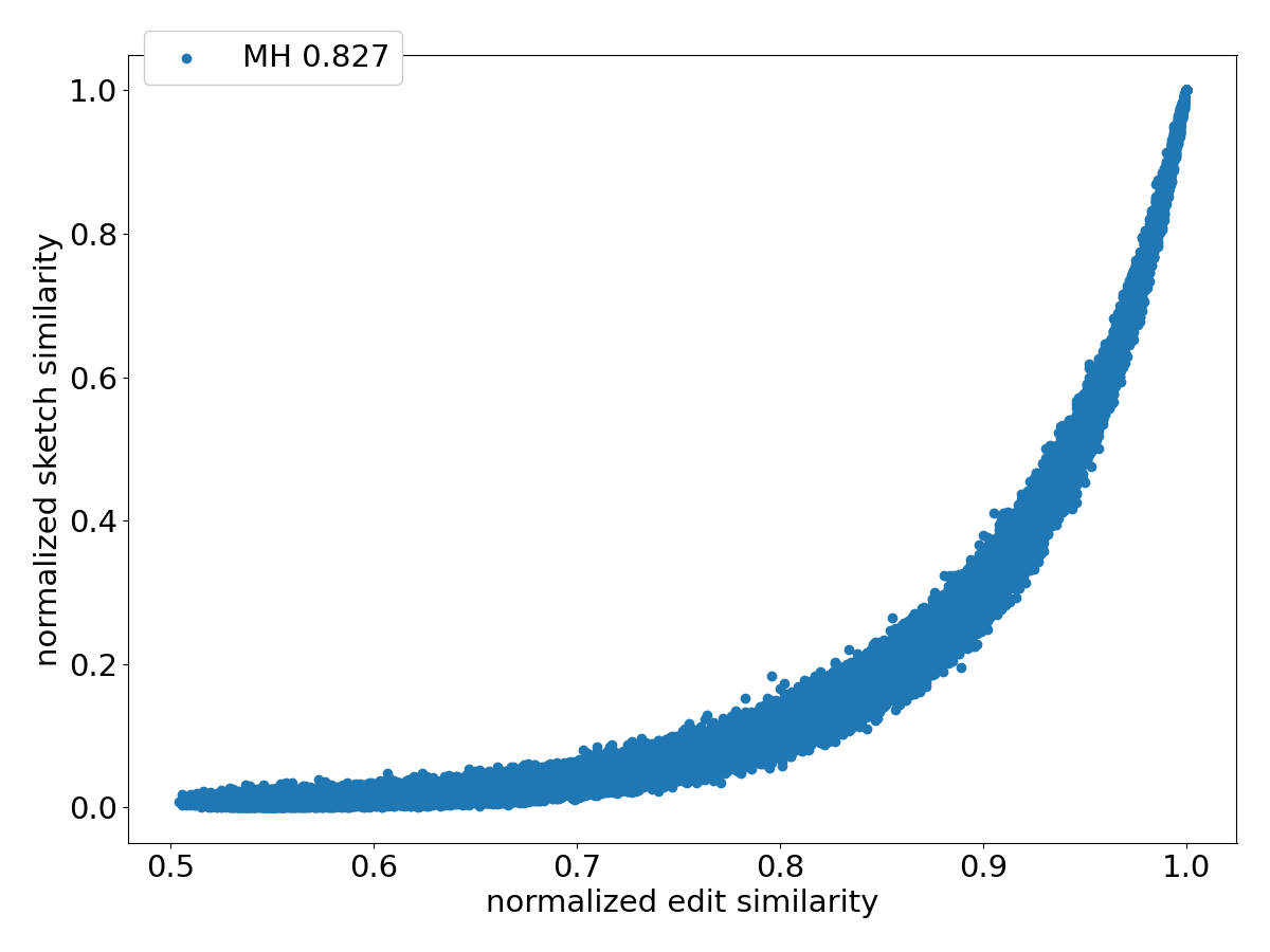
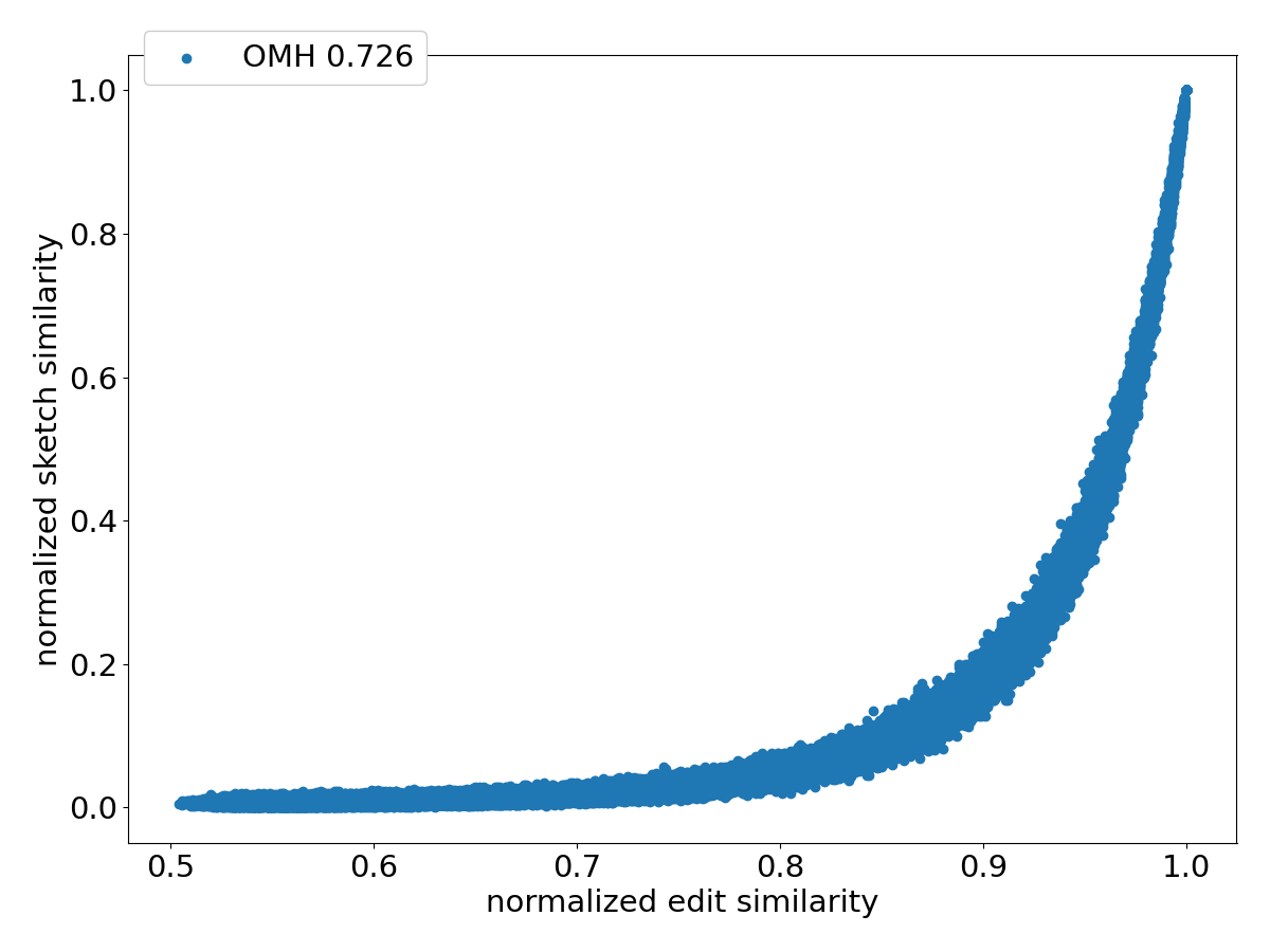
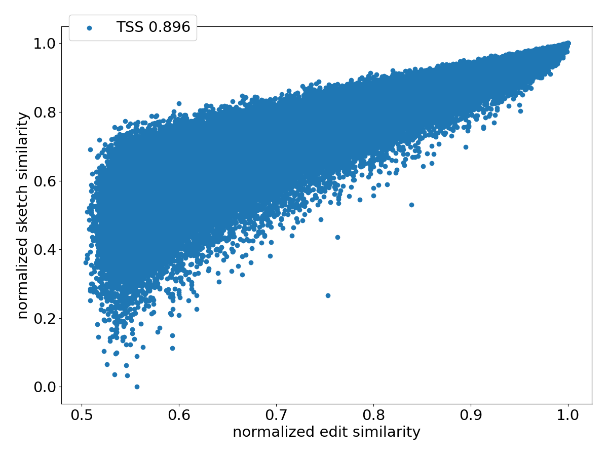
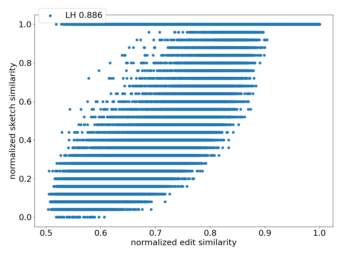
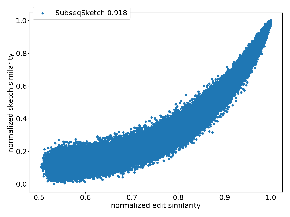
Figure 4 shows the scatter plots of all the pairs under different sketching methods. Observe that SubseqSketch achieves the best Pearson correlation. Both MH and OMH are good estimators for sequences with high edit similarities but struggle to distinguish dissimilar sequences with edit similarity between and . The TSS and LH similarities show a visually more linear relationship with the edit similarity and consequently exhibit higher Pearson correlations than MH and OMH. But they both suffer from extremely large variance, especially for dissimilar sequences, which makes it difficult to interpret their estimation in practical applications. SubseqSketch strikes a balance between the ability to estimate the full range of edit similarity and the estimation variance.
As with other sketching methods, the variance of SubseqSketch can be reduced by using a larger sketch. For all the experiments, we measure the size of a sketch as the number of entries in it (sometimes called its dimension), and all methods are configured to produce the same number of entries (except for TSS, which we follow the suggestion in [12] even though it produces a larger sketch). However, in real applications, the actual space needed to store the sketches is a more relevant measure. Recall that each entry of SubseqSketch can be stored in 4 bits (ref. Section 2.4) which is four times smaller than an entry of MH (16 bits for ), six times smaller than OMH (24 bits for and ), and eight times smaller than TSS and LH (32-bit float/int). Thus, given a fixed amount of disk space, SubseqSketch can utilize more testing sequences than the number of -mers MH or OMH can select, thereby achieving a similar or better variance. In the experiments, we do not exploit this practical advantage, opting instead to use the same number of sketch entries across all methods.
3.2 Nearest neighbor search
The task of nearest neighbor search involves finding the top- most similar sequences for a query among a large database. It has numerous applications in bioinformatics, including metagenomic classification and gene function prediction. Because computing the exact edit distance between the query and every sequence in the database is computationally prohibitive, a common approach is to embed database sequences into a well-studied metric space where efficient nearest neighbor indexing is readily available (for example, the hierarchical navigable small world index [18]). The query is embedded in the same space, and the nearest neighbors identified by the index serve as approximations to the true nearest neighbors under edit distance. Given the high correlation between SubseqSketch and edit distance, we demonstrate in this section that it can serve as an embedding method and yields improved nearest neighbor search performance.
In this experiment, we restrict our comparison to CNN-ED [5], a deep convolutional neural network model for sequence embedding that has been shown to outperform non-machine learning approaches such as CGK embedding [4]. For evaluation purpose, the CNN-ED pipeline splits an input dataset into three disjoint sets: a training set with sequences, a query set with sequences, and a base set containing the remaining sequences. It computes pairwise edit distances among the training set to generate training labels. After the model is trained, it generates embeddings for all sequences in the query and base set. All-vs-all embedding distances as well as the ground-truth edit distances between the query set and the base set are then computed so that the top- neighbors identified by the embedding can be compared with the top- neighbors according to the edit distance. Following this pipeline, we apply SubseqSketch to all sequences in the query and base set, and report top- neighbors using the all-vs-all sketch distances. It is worth noting that, unlike in practical applications, indexing is omitted in this experiment to enable a direct comparison of the embedding/sketching quality, independent of variations in index accuracy.
We show results on two widely used datasets GEN50kS and GEN20kL from [29] which are also benchmarked in the CNN-ED paper. The GEN50kS dataset contains sequences with an average length . The GEN20kL dataset contains sequences with an average length .
In Figure 5 and Figure 6, we plot the commonly used recall-item curves for both SubseqSketch and CNN-ED. For a figure labeled top-, the nearest neighbors of a query in the base set according to the edit distances are considered true neighbors. The horizontal axis represents the number of neighbors (items) each method is allowed to report (according to their respective sketch/embedding distances) and the vertical axis marks the fraction of true neighbors being reported (recall). The CNN-ED pipeline presents full-range results – from reporting a single item to reporting all items – which, while not practical for typical use cases (where only the top- neighbors are retrieved), allows for plotting complete performance curves.
The CNN-ED results are obtained by the implementation of [5], which we trained for 50 epochs following the reported hyperparameters in the original paper. For a fair comparison, SubseqSketch is configured to produce vectors of the same length as the reported embedding dimensions of CNN-ED. Observe that SubseqSketch consistently outperforms CNN-ED by a large margin. This is a surprising result. It is commonly believed (which is often, though not always, justified) that machine learning models can outperform traditional algorithmic methods because the models can learn data-dependent features that the data-oblivious algorithms cannot take advantage of. In [5], the CGK embedding [4] was shown to produce a worse result than CNN-ED on this task, even though it is an edit distance embedding with theoretical guarantees. Our result here demonstrates that there is a gap between theoretical bounds and practical performance which warrants further investigation. In particular, we conjecture that SubseqSketch can also provide some guarantees on the distortion as a randomized embedding function for the edit distance, though a theoretical proof seems difficult.
3.3 Phylogeny reconstruction
Phylogeny reconstruction is another task commonly used to evaluate the performance of sketching methods. Given a set of biologically related genomes, the goal is to build a phylogeny on them based on pairwise similarities/distances estimated by the sketches. The result can then be compared with a ground truth tree constructed from some biological model or multiple sequence alignment. We test on two datasets for this task: one is a simulation of a simple mutation model similar to that used in [20]; the other is a set of 29 assembled E. coli genome sequences collected in [28].
The simulation aims to model both point mutations and mobile genomic elements, commonly found in bacterial genome rearrangements, known as insertion sequences (IS). The simulated sequences form a perfect binary tree. The root of the tree is a random sequence of length ; it is considered as the -th generation genome. To obtain the -th generation, each sequence in the -th generation produces two children genomes by independent and random point mutations with mutation rate . Then a random IS of length is inserted at a random position for each newly generated -th generation genomes. Note that the IS is shared among all sequences in the same generation, but the inserting positions can be different. See Figure 7 for an illustration. Although simple and somewhat unrealistic, this model produces a solid ground truth phylogeny and allows us to investigate the effectiveness of different sketching methods to recover the mixed history of point mutations and large insertion events.
Each method computes a pairwise distance matrix for all sequences in each generation. The matrices are used to build the phylogenies with the neighbor-joining algorithm implemented in the biotite package [13]. The normalized Robinson-Foulds (nRF) distances between the constructed trees and the ground truth tree are then calculated with the ETE toolkit [10]. The nRF distance measures the dissimilarity of branching patterns between two trees and ignores branch lengths. A value of means the two phylogenies have the identical tree topology, whereas a value of indicates the two trees are maximally dissimilar.
Figure 8 shows the nRF distances achieved by each method on progressively larger inputs from the simulated dataset. The horizontal label means all the sequences from the -th generation are used as input sequences. Not surprisingly, pairwise edit distance (ED) most accurately captures the mutation history, at the cost of significantly longer computation time (see Figure 9). Among the sketching methods, SubseqSketch constructs the best phylogeny for generation and larger inputs. Furthermore, the nRF distances obtained by SubseqSketch exhibits a strong correlation with those achieved by the exact edit distances, indicating it can be used as a faithful approximation of the expensive edit calculation. In contrast, although MH and OMH produce trees with smaller nRF distances for the smaller input sets, they both show some inverse relation with the nRF using edit distances (e.g., from generation to , the nRF distances of trees constructed by edit distance increased, but the nRF distances for MH decreased; similarly from generation to for OMH). LH is omitted from this experiment because its implementation choice for boundary handling tends to assign the maximum similarity score to pairs sharing a short matching suffix (see the line at normalized similarity score in Figure 4). While this may be appropriate for the overlap detection task that LH is designed for, it hinders accurate phylogeny reconstruction on our datasets.
We also plot the running time of each sketching method in Figure 9 to demonstrate the efficiency of SubseqSketch. As expected, all the sketching methods are much faster than computing the all-vs-all exact edit distances. Among them, SubseqSketch is consistently the fastest, regardless of the number of input sequences. More specifically, SubseqSketch achieves a speedup compared to the second fastest method (MH).
For testing on a real dataset, 29 assembled E. coli genome sequences are obtained from the AFproject [30], a benchmark project for alignment-free sequence analysis tools. It provides a web interface where the phylogenies can be computed from the uploaded distance matrices. The nRF distances are then reported by comparing the resulting trees against a ground truth tree built from multiple sequence alignment. It also provides the normalized Quartet Distance (nQD) as an additional measure for topological disagreement.
Results on this E. coli dataset are summarized in Table 3. On the AFproject website, nearly 100 tools (include different configurations for the same tool) are ranked based on the nRF distance. SubseqSketch is ranked 7th and there are 12 tools that achieve smaller nRF distances due to ties. It is worth pointing out that the higher ranked ones are tools designed specifically for the task of phylogeny reconstruction, which are often based on some sketching method but also apply biological and algorithmic heuristics to adjust the sketch distance matrix. Since SubseqSketch is a sketching method rather than a complete tool for phylogeny, here we aim to evaluate the sketch quality without those adjustments. With the unadjusted distance matrices, SubseqSketch constructs the best phylogeny (closest to the ground truth) among MH, OMH, and TSS.
In this task, since there are only genomes, we can afford to sample the testing sequences from the input to further improve the quality of SubseqSketch. Because the inputs are all closely related, this sampling strategy also enables us to use a much larger token size to achieve an even better result than the recommended . From Table 3, it is evident that setting significantly improves accuracy.
| Method | RF | nRF | nQD | Rank |
|---|---|---|---|---|
| MH | 30 | 13 | ||
| OMH | 30 | 13 | ||
| TSS | 40 | 17 | ||
| SubseqSketch () | 22 | 9 | ||
| SubseqSketch () | 18 | 7 |
4 Discussion
We presented SubseqSketch, a subsequence-based sketching method that is both effective and efficient at sequence similarity estimation. Comparing to the widely used MH, OMH, TSS, and LH sketches, SubseqSketch requires smaller space, is faster to compute, and achieves a stronger correlation with the edit similarity. It delivers strong performance in two alignment-free tasks: nearest neighbor search and phylogeny reconstruction. In particular, it outperforms a machine learning edit distance embedding model by a large margin which suggests our method indeed captures critical features of the sequences being sketched.
A large body of work that we intentionally excluded from our experiments consists of seeding-based methods. The simplest seeds are -mers, representing fixed-length consecutive exact matches in the sequences. More advanced -mer selection schemes exist, such as minimizer [25, 19], syncmer [6] and -min-mer [7]. Seeds sampled from subsequences, either with limited patterns such as spaced seed [3, 16] and strobemer [23, 17, 24], or fully unrestricted such as SubseqHash [15, 14], have been shown to deliver better performance but are usually more expensive to compute. While both sketching and seeding utilize some common techniques, for example, the minimizer seeds are obtained by applying MH [2] on each window, they differ significantly in their goals, representations and usage. Seeding methods aim to identify local regions of similarity between sequences, providing fine-grained information about where and how sequences resemble each other. This often comes at the cost of increased memory footprint and computational overhead. Specifically, seeding methods typically extract seeds from a relatively small sliding window over a longer input sequence. By generating one or more seeds from each overlapping window111There also exist seeding schemes without a window guarantee, such as syncmer [6]., the number of seeds for a sequence of length is usually . In contrast, sketching methods prioritize efficiency by transforming sequences into compact, low-dimensional representations that enable fast, global similarity estimation. For example, an E. coli genome with several million base pairs is condensed to a length vector by each sketching method in the above experiment. Unlike seeds, which are often used temporarily during computation and then discarded, sketches are typically stored and reused, serving as compact indices in databases containing vast numbers of sequences.
There are numerous interesting directions that call for further investigations. From the theoretical perspective, a deeper understanding of SubseqSketch, and subsequence-based features in general, can be beneficial for better algorithmic designs as well as guiding practical applications. For example, recent work [1] has shown that pattern matching with gaps, a problem closely related to finding tokenized subsequences, can be solved in strongly subquadratic time, making it a promising variant for improving SubseqSketch. Many methods compared in the experiments come with theoretical guarantees: MH is an unbiased estimator for the Jaccard similarity; OMH is a locality-sensitive hashing (LSH) family for the edit distance; and CGK is an embedding for the edit distance with a quadratic distortion. Given the superior performance of SubseqSketch against these methods, it is natural to consider what bounds can be proved on it. More specifically, we are curious if SubseqSketch is an LSH, and if so, does it offer better hash collision probabilities? Or is it an embedding with provable small distortion for the edit distance? In that case, study the relation between its parameters and the achieved distortion can help to make informed decisions in practical use.
On the application side, there are several potential approaches to enhance SubseqSketch. For example, Mash [21] is a popular tool for genome distance estimation. It is based on MH whose estimation does not exhibit the strongest correlation with edit distance. However, by applying a simple Poisson model to adjust the MH score [21], Mash produces a distance that closely approximates the mutation rate on real datasets. Since SubseqSketch starts with a more accurate estimation, it is reasonable to believe that similar techniques can be applied to further improve its performance.
A related question concerns the similarity function used by SubseqSketch. The cosine similarity was chosen for its effectiveness and simplicity. While it matches our intuition that sketches of similar sequences should have near identical corresponding entries and therefore should be roughly pointing to the same direction in the sketch vector space, the cosine similarity explicitly ignores the magnitude of the vectors. In the extreme case, a sketch full of 1’s is considered to have the maximum similarity with another sketch full of 10’s. This greatly diverges from the designed meaning of the SubseqSketch entries – the first sequence barely contains any testing sequences whereas the second contains large portions of each testing sequence – they must be very different! Exploring different similarity functions that can better incorporate the expected interpretation of the entries can therefore potentially make SubseqSketch more accurate.
Yet another observation is that SubseqSketch is sensitive for globally well-aligned sequences but can struggle with ones that only share meaningful local alignments. For example, we cannot expect a genome comprising millions of base pairs to produce a SubseqSketch similar to that of a 100-base-pair short read. Other sketching methods such as MH also suffer from these situations and special variants such as FracMinHash [11] are designed to handle them differently. As another example, in building overlap graphs for genome assembly, one needs to identify overlapping pairs of sequences that contain additional unaligned prefixes and suffixes. Suppose that the tail of sequence overlaps with the head of sequence . Since SubseqSketch tests for subsequences from left to right and stops immediately when the next token cannot be found, the sketches will be disproportionally skewed: because does not have the beginning part of , testing sequences fully live inside can produce 0’s for , even if contains long suffixes of them. We hope to see diverse adaptations of SubseqSketch designed to address these various challenges.
References
- [1] Aranya Banerjee, Daniel Gibney, and Sharma V. Thankachan. Longest Common Substring with Gaps and Related Problems. In Timothy Chan, Johannes Fischer, John Iacono, and Grzegorz Herman, editors, 32nd Annual European Symposium on Algorithms (ESA 2024), volume 308 of Leibniz International Proceedings in Informatics (LIPIcs), pages 16:1–16:18, Dagstuhl, Germany, 2024. Schloss Dagstuhl – Leibniz-Zentrum für Informatik. doi:10.4230/LIPIcs.ESA.2024.16.
- [2] Andrei Z Broder. On the resemblance and containment of documents. In Proceedings. Compression and Complexity of SEQUENCES 1997 (Cat. No. 97TB100171), pages 21–29. IEEE, 1997. doi:10.1109/SEQUEN.1997.666900.
- [3] Andrea Califano and Isidore Rigoutsos. FLASH: A fast look-up algorithm for string homology. In Proceedings of IEEE Conference on Computer Vision and Pattern Recognition (CVPR’93), pages 353–359. IEEE, 1993. doi:10.1109/CVPR.1993.341106.
- [4] Diptarka Chakraborty, Elazar Goldenberg, and Michal Koucký. Streaming algorithms for embedding and computing edit distance in the low distance regime. In Daniel Wichs and Yishay Mansour, editors, Proceedings of the 48th Annual ACM SIGACT Symposium on Theory of Computing, STOC 2016, Cambridge, MA, USA, June 18-21, 2016, pages 712–725. ACM, 2016. doi:10.1145/2897518.2897577.
- [5] Xinyan Dai, Xiao Yan, Kaiwen Zhou, Yuxuan Wang, Han Yang, and James Cheng. Convolutional embedding for edit distance. In Proceedings of the 43rd international ACM SIGIR conference on Research and Development in information retrieval, pages 599–608, 2020. doi:10.1145/3397271.3401045.
- [6] Robert Edgar. Syncmers are more sensitive than minimizers for selecting conserved k-mers in biological sequences. PeerJ, 9:e10805, 2021. doi:10.7717/peerj.10805.
- [7] Barış Ekim, Bonnie Berger, and Rayan Chikhi. Minimizer-space de Bruijn graphs: Whole-genome assembly of long reads in minutes on a personal computer. Cell Systems, 12(10):958–968, 2021. doi:10.1016/j.cels.2021.08.009.
- [8] Martin C Frith, Jim Shaw, and John L Spouge. How to optimally sample a sequence for rapid analysis. Bioinformatics, 39(2):btad057, 2023. doi:10.1093/bioinformatics/btad057.
- [9] Grant Greenberg, Aditya Narayan Ravi, and Ilan Shomorony. Lexichash: sequence similarity estimation via lexicographic comparison of hashes. Bioinformatics, 39(11):btad652, October 2023. doi:10.1093/bioinformatics/btad652.
- [10] Jaime Huerta-Cepas, François Serra, and Peer Bork. Ete 3: Reconstruction, analysis, and visualization of phylogenomic data. Molecular Biology and Evolution, 33(6):1635–1638, February 2016. doi:10.1093/molbev/msw046.
- [11] Luiz Irber, Phillip T Brooks, Taylor Reiter, N Tessa Pierce-Ward, Mahmudur Rahman Hera, David Koslicki, and C Titus Brown. Lightweight compositional analysis of metagenomes with fracminhash and minimum metagenome covers. bioRxiv, pages 2022–01, 2022. doi:10.1101/2022.01.11.475838.
- [12] Amir Joudaki, Gunnar Ratsch, and André Kahles. Fast alignment-free similarity estimation by tensor sketching. bioRxiv, 2020. doi:10.1101/2020.11.13.381814.
- [13] Patrick Kunzmann, Tom David Müller, Maximilian Greil, Jan Hendrik Krumbach, Jacob Marcel Anter, Daniel Bauer, Faisal Islam, and Kay Hamacher. Biotite: new tools for a versatile python bioinformatics library. BMC bioinformatics, 24(1):236, 2023. doi:10.1186/s12859-023-05345-6.
- [14] Xiang Li, Ke Chen, and Mingfu Shao. Efficient seeding for error-prone sequences with subseqhash2. bioRxiv, pages 2024–05, 2024. doi:10.1101/2024.05.30.596711.
- [15] Xiang Li, Qian Shi, Ke Chen, and Mingfu Shao. Seeding with minimized subsequence. Bioinformatics, 39(Supplement_1):i232–i241, June 2023. doi:10.1093/bioinformatics/btad218.
- [16] Bin Ma, John Tromp, and Ming Li. Patternhunter: faster and more sensitive homology search. Bioinformatics, 18(3):440–445, 2002. doi:10.1093/bioinformatics/18.3.440.
- [17] Benjamin Dominik Maier and Kristoffer Sahlin. Entropy predicts sensitivity of pseudorandom seeds. Genome Research, 33(7):1162–1174, 2023. doi:10.1101/gr.277645.123.
- [18] Yu A Malkov and Dmitry A Yashunin. Efficient and robust approximate nearest neighbor search using hierarchical navigable small world graphs. IEEE transactions on pattern analysis and machine intelligence, 42(4):824–836, 2018. doi:10.1109/TPAMI.2018.2889473.
- [19] Guillaume Marçais, Dan DeBlasio, and Carl Kingsford. Asymptotically optimal minimizers schemes. Bioinformatics, 34(13):i13–i22, 2018. doi:10.1093/bioinformatics/bty258.
- [20] Guillaume Marçais, Dan DeBlasio, Prashant Pandey, and Carl Kingsford. Locality-sensitive hashing for the edit distance. Bioinformatics, 35(14):i127–i135, 2019. doi:10.1093/bioinformatics/btz354.
- [21] Brian D Ondov, Todd J Treangen, Páll Melsted, Adam B Mallonee, Nicholas H Bergman, Sergey Koren, and Adam M Phillippy. Mash: fast genome and metagenome distance estimation using minhash. Genome biology, 17:1–14, 2016. doi:10.1186/s13059-016-0997-x.
- [22] Will PM Rowe. When the levee breaks: a practical guide to sketching algorithms for processing the flood of genomic data. Genome Biology, 20:1–12, 2019. doi:10.1186/s13059-019-1809-x.
- [23] Kristoffer Sahlin. Effective sequence similarity detection with strobemers. Genome Research, 31(11):2080–2094, 2021. doi:10.1101/gr.275648.121.
- [24] Kristoffer Sahlin. Strobealign: flexible seed size enables ultra-fast and accurate read alignment. Genome Biology, 23(1):1–27, 2022. doi:10.1186/s13059-022-02831-7.
- [25] Saul Schleimer, Daniel S Wilkerson, and Alex Aiken. Winnowing: local algorithms for document fingerprinting. In Alon Y. Halevy, Zachary G. Ives, and AnHai Doan, editors, Proceedings of the 2003 ACM SIGMOD International Conference on Management of Data (SIGMOD/PODS’03), pages 76–85. ACM, 2003. doi:10.1145/872757.872770.
- [26] Wei Shen and Zamin Iqbal. Lexicmap: efficient sequence alignment against millions of prokaryotic genomes. bioRxiv, pages 2024–08, 2024. doi:10.1101/2024.08.30.610459.
- [27] Yan Song, Haixu Tang, Haoyu Zhang, and Qin Zhang. Overlap detection on long, error-prone sequencing reads via smooth q-gram. Bioinformatics, 36(19):4838–4845, 2020. doi:10.1093/bioinformatics/btaa252.
- [28] Huiguang Yi and Li Jin. Co-phylog: an assembly-free phylogenomic approach for closely related organisms. Nucleic Acids Research, 41(7):e75–e75, January 2013. doi:10.1093/nar/gkt003.
- [29] Haoyu Zhang and Qin Zhang. Embedjoin: Efficient edit similarity joins via embeddings. In Proceedings of the 23rd ACM SIGKDD international conference on knowledge discovery and data mining, pages 585–594, 2017. doi:10.1145/3097983.3098003.
- [30] Andrzej Zielezinski, Hani Z Girgis, Guillaume Bernard, Chris-Andre Leimeister, Kujin Tang, Thomas Dencker, Anna Katharina Lau, Sophie Röhling, Jae Jin Choi, Michael S Waterman, et al. Benchmarking of alignment-free sequence comparison methods. Genome biology, 20:1–18, 2019. doi:10.1186/s13059-019-1755-7.