Shortest Paths in Multimode Graphs

Abstract
In this work we study shortest path problems in multimode graphs, a generalization of the min-distance measure introduced by Abboud, Vassilevska W. and Wang in [SODA’16]. A multimode shortest path is the shortest path using one of multiple “modes” of transportation that cannot be combined. This represents real-world scenarios where different modes are not combinable, such as flights operated by different airline alliances. The problem arises naturally in machine learning in the context of learning with multiple embedding. More precisely, a -multimode graph is a collection of graphs on the same vertex set and the -mode distance between two vertices is defined as the minimum among the distances computed in each individual graph.
We focus on approximating fundamental graph parameters on these graphs, specifically diameter and radius. In undirected multimode graphs we first show an elegant linear time 3-approximation algorithm for 2-mode diameter. We then extend this idea into a general subroutine that can be used as a part of any -approximation, and use it to construct a 2 and 2.5 approximation algorithm for 2-mode diameter. For undirected radius, we introduce a general scheme that can compute a 3-approximation of the -mode radius for any and runs in near linear time in the case of . In the directed case we establish an equivalence between approximating 2-mode diameter on DAGs and approximating the min-diameter, while for general graphs we develop novel techniques and provide a linear time algorithm to determine whether the diameter is finite.
We also develop many conditional fine-grained lower bounds for various multimode diameter and radius approximation problems. We are able to show that many of our algorithms are tight under popular fine-grained complexity hypotheses, including our linear time 3-approximation for -mode undirected diameter and radius. As part of this effort we propose the first extension to the Hitting Set Hypothesis [SODA’16], which we call the -Hitting Set Hypothesis. We use this hypothesis to prove the first parameterized lower bound tradeoff for radius approximation algorithms.
Keywords and phrases:
Graph Algorithms, Shortest Paths, Diameter, Radius, Fine-Grained ComplexityFunding:
Yael Kirkpatrick: NSF Graduate Research Fellowship under Grant No. 2141064.Copyright and License:
2012 ACM Subject Classification:
Theory of computation Graph algorithms analysisAcknowledgements:
The authors would like to thank Asaf Etgar, Jenny Kaufmann and Surya Mathialagan for helpful discussions.Editors:
Paweł Gawrychowski, Filip Mazowiecki, and Michał SkrzypczakSeries and Publisher:
1 Introduction
The study of shortest paths algorithms in directed graphs has introduced various distance measures. The most standard notion of distance between two vertices and is the minimum length of a path from to , . This asymmetric one-way notion of distance is not always the most natural. In some applications the roundtrip distance , defined by Cowen and Wagner [8], is most useful, since unlike its one-way counterpart, it is a metric.
In directed acyclic graphs (DAGs), however, both the standard notion of distance and the roundtrip notion produce infinite distances for all or a large fraction of the distance pairs. A more useful notion of distance in this case was defined by Abboud, Vassilevska W. and Wang [1]. In this work they introduced the min-distance, defined as . Under one-way distance or roundtrip distance, almost all points in a DAG have infinite eccentricity. Introducing min-distance opened an avenue of research which lead to intricate algorithms for computing or approximating min-diameter, radius and eccentricities in DAGs [1, 9] as well as for general graphs [3, 7, 12].
One real-world motivation for studying the min-distance problem is computing the optimal location for a hospital, as one has the choice of either going to the hospital or having a doctor come to them. The min-distance therefore measures the fastest way to receive care and the point with smallest min-eccentricity in the graph functions as the optimal location for a hospital. Imagine now that the doctor can take a helicopter, whereas a patient can only take a cab to the doctor. Then the two routes are no longer part of the same graph - the routes by which a helicopter can travel are very different from those available to a taxi. The new distance between the patient and the doctor is now the minimum between the distances in two different graphs.
Consider another common scenario. We want to fly from city to city . We can take any valid itinerary, except that each itinerary needs to stay within the same airline alliance. Now the fastest flight time is the minimum of the distances over several different “graphs”, one for each airline alliance. All of these graphs share a vertex set representing the different cities, while each graph has edges representing the flights of a single airline alliance.
Let us formalize a new shortest paths problem that captures both scenarios. Consider a collection of graphs over the same vertex set . Let their edge sets be . Together they form a “-multimode graph” . One can associate each with a “mode of transportation”, where these modes are separate and cannot be combined.
The -mode distance between two vertices in a -multimode graph is defined as
where is the distance in the graph . Intuitively, is the length of the shortest path connecting and using a single mode of transportation.
The -mode distance naturally arises in practice in the context of multiple embeddings in machine learning (see [21, 15, 18] and many more). In many scenarios, given a high dimensional data set, there is no clear distance function that accurately captures semantic relationships within the data. To address this, deep learning is now commonly used to obtain a data embedding that encodes semantic information. As research in this field advances, we observe a proliferation of embeddings which can vary due to differences in network architecture, learning paradigms or training data, to name a few. This results in a single set of data points with multiple sets of edges representing distances in the different embeddings spaces. For every pair of points we are interested in the embedding in which they are closest together and often care about finding a pair of points which are furthest apart in all embeddings (i.e. computing the -mode diameter) or a point which is closest to all others in some embedding (i.e. computing the -mode radius).
Let us first consider the All-Pairs Shortest Paths (APSP) problem in -multimode graphs on vertices: compute the -mode distance between all pairs of vertices of . One can always run any APSP algorithm on each separately, resulting in a running time which is times that of the standard APSP algorithm. This approach will also trivially compute the -mode radius of the multimode graph. In fact, we show that in general no algorithm can have polynomial improvements over this trivial solution.
Theorem 1.
Under the APSP hypothesis [17], no time algorithm can solve -mode APSP or -mode radius for any .
While it is clear for APSP that one can compute all -multimode distances by solving instances of APSP separately on each graph, it is no longer obvious how to solve -multimode radius or diameter using algorithms that compute the radius or diameter in a standard graph.
To illustrate why the -mode diameter is not directly related to the standard diameters of the individual graphs , denote the diameter of by and let be such that . Similarly, denote the diameter of by and let be such that . We cannot merely take the minimum of to get the diameter in the multimode graph . This is because it could be that and so that the multimode distance between and is not but rather and similarly for and . The multimode diameter can be the distance between some completely different pair of vertices and thus can be arbitrarily smaller than both and . It could even be the case that are infinite, while the multimode diameter is finite.
However, if we wish to compute the exact -mode diameter or radius of a -multimode undirected graph, we show that we can in fact use any algorithm for computing standard diameter or radius in a blackbox way.
Theorem 2.
If there exists a time algorithm for computing the diameter/radius of a weighted, undirected graph with -nodes and -edges, then there exists an algorithm for computing the -mode diameter of a -multimode undirected graph in time .
The proofs of both Theorem 1 and Theorem 2 follows from a straightforward application of standard techniques. We therefore defer their proofs to the full version of this work. We instead turn our focus to approximating these parameters.
There exists a plethora of algorithms and conditional lower bounds for approximating diameter and radius under both the standard notion of (directed or undirected) distance and the min-distance measure [2, 1, 7, 9, 10, 11, 6, 16, 4, 13]. As the -multimode distance generalizes both these distance measures, we would like to develop approximation algorithms and prove tight conditional lower bounds for approximating diameter and radius in the multimode setting as well.
The known fine-grained hardness results for the min-distance and standard diameter, radius and eccentricities would trivially carry over for the multimode distance case (as it generalizes both). We are thus interested in when stronger hardness is possible, and when similar approximation algorithms can be attained.
Devising approximation algorithms for the min-distance measure is particularly difficult and therefore significantly new techniques had to be developed over the standard diameter ones (see e.g. [12, 7, 9]). The main difficulty lies in the fact that the triangle inequality no longer holds: it could be that and but , as in the graph with vertices and edges . This difficulty persists and is even more prominent in the multimode distance setting, as now the various graphs that represent modes of transportation may not share any edges. We can therefore expect that the distance parameters of interest can be even more difficult to approximate.
1.1 Our results
We develop various new techniques that work in the multimode distance setting, both for directed and undirected graphs, and for fine-grained conditional lower bounds. Table 1 summarizes our results. Here we present some highlights.
The runtimes marked with assume .
| Approx. | Runtime | Comments | Reference | ||||
| Undirected -mode Diameter Upper Bounds | |||||||
| Weighted | Theorem 9 | ||||||
| Weighted. | Theorem 13 | ||||||
|
See full version | ||||||
|
See full version | ||||||
| Undirected -mode Diameter Lower Bounds (Under SETH) | |||||||
| Unweighted | See full version | ||||||
| Unweighted. | See full version | ||||||
| Any | Unweighted. | See full version | |||||
| Directed -mode Diameter Upper Bounds | |||||||
| Weighted. | See full version | ||||||
| Weighted DAG. | See full version | ||||||
| Unweighted DAG. | See full version | ||||||
| Directed -mode Diameter Lower Bounds (Under SETH) | |||||||
| Unweighted. | See full version | ||||||
| Any | Unweighted DAG. | See full version | |||||
| Undirected -mode Radius Upper Bounds | |||||||
|
Theorem 14 | ||||||
| Undirected -mode Radius Lower Bounds (Under the HS Hypothesis) | |||||||
| Unweighted. | See full version | ||||||
|
See full version | ||||||
| Any | Unweighted. | See full version | |||||
| Directed -mode Radius Upper Bounds for DAGs | |||||||
| Weighted DAG. | See full version | ||||||
| Directed -mode Radius Lower Bounds (Under the HS Hypothesis) | |||||||
| Any | Unweighted. | See full version | |||||
| Unweighted DAG. | See full version | ||||||
| Any | Unweighted DAG. | See full version | |||||
Our hardness results are based on the Strong Exponential Time Hypothesis (SETH) [14, 5] and the Hitting Set Hypothesis [1] (see also [19]). We further extend the Hitting Set Hypothesis to the stronger -Hitting Set Hypothesis. Based on this new hypothesis we are able to obtain a lower bound tradeoff for approximating the -mode radius. As the introduction of the Hitting Set Lemma in [1] allowed for the proof of the first lower bounds on radius approximation, we hope this extension will enable future work on lower bound tradeoffs for radius in various distance frameworks.
Theorem 3.
Let . Under SETH, there can be no time (for ) algorithm that achieves any finite multiplicative approximation for the -mode diameter in directed unweighted -edge multimode graphs, even if all graphs in the multimode graph are DAGs.
The result appears as Theorem 5.3 in the full version of the text. It implies that, under SETH, to get any approximation algorithm for directed multimode diameter, even for DAGs, one must focus on or . The case is just the standard diameter problem, and so we consider the case where next.
For -mode diameter in directed graphs we provide (1) a near-linear time algorithm that can decide whether the diameter is finite, and (2) a near-linear time -approximation algorithm for the case when both graphs in the multimode graph are DAGs. Both of these results are tight, in the sense that for such results are impossible under SETH. The results appear in the full version.
For -mode diameter and radius in undirected graphs we obtain several tight results as well. Here are two highlights:
Theorem 4.
For every constant , there is an time111As is standard, hides polylogarithmic factors. -approximation algorithm for the radius of -edge undirected -multimode graphs. This is tight under the -Hitting Set Hypothesis, in that no -approximation is possible in time, even for .
This algorithmic result is stated in Theorem 14 while the lower bound appears in the full version. It achieves the conditionally best possible result for radius in near-linear time.
Theorem 5.
Under SETH, there can be no -approximation algorithm for diameter running in time for for -edge -mode undirected unweighted graphs. If ,222Here denotes the fast matrix multiplication exponent, [20]. there is an time algorithm that achieves a -multiplicative, -additive approximation to the diameter in -edge, -node undirected -multimode graphs.
This result appears in the full version. Up to the small additive error, the approximation algorithm is optimal due to the SETH-based lower bound. The running time of the algorithm is still faster than , even with the current bound on .
1.2 Technical Overview
In this subsection we describe an outline of some of our results, and highlight their connections to other, well studied problems.
Approximating Undirected 2 and 3 Mode Diameter
Our first result is a simple, linear time 3-approximation for 2-mode diameter. Given a threshold , we would like to either show that the 2-mode diameter is less than or find a pair of points whose 2-mode distance is greater than , meaning and .
To find such a pair, run BFS from an arbitrary point . Let be the points within distance of in and let be the points within distance of in . If any vertex is contained in neither nor , then it has multimode distance greater than from and we are finished.
Next, run BFS from (as a set) in to identify the vertices in that have distance in from all vertices in . Similarly, run BFS from in to identify all vertices in that have distance in from all vertices in . If there exists a pair of vertices such that and then the multimode distance of is greater than and we are done. Otherwise, we can show that any pair of points has multimode distance , and thus the 2-mode diameter is . Indeed, if then using a path through in . Similarly, if then . Otherwise, we can assume w.l.o.g that and . Then there exists a point such that . Now, following a path in from to to to we have that . Thus, for any pair of vertices we have .
This completes our 3-approximation for undirected 2-mode diameter in linear time. Next we generalize this approach to a subroutine that can be used for any -approximation for . Informally, we take to be the neighborhood in of some point and to be the neighborhood in of some point . We perform a similar search, running BFS from the set in and from in to find a pair of points in that is far apart in both graphs. In order to conclude that the graph has a small diameter in the case that we do not find a pair of large distance, we need to consider all pairs where is in the neighborhood of a vertex and is in the neighborhood of the same vertex . This results in a subroutine that, given a point with small and neighborhoods, we can compute a -approximation to the 2-mode diameter. For details see Lemma 12.
We can now use this idea to construct -approximation algorithms using a classic large-small neighborhoods tradeoff. We show two ways in which to use this subroutine in a complete algorithm, obtaining a 2-approximation and a 2.5-approximation.
For our 2-approximation, if we have a point with small and neighborhoods, we use the aforementioned subroutine. Otherwise, all vertices have a large or neighborhood, including the endpoints of the diameter. We leverage this fact and sample a hitting set, hitting the or neighborhood of a diameter endpoint. For every point in this hitting set, we compute the set of points of distance from in and the set of points of distance from in . We show that if the 2-mode diameter is and hits the neighborhood of a diameter endpoint, then the ST-diameter of the sets in will be . We can therefore use an ST-diameter approximation algorithm in a black box way to obtain our desired approximation.
To obtain our 2.5-approximation we use a similar approach, leveraging a blackbox ST-diameter 2.5-approximation. Using a slightly different method, we apply the simple 3-approximation of ST-diameter to turn our linear time 2-mode diameter approximation into an approximation for 3-mode diameter, incurring only poly-logarithmic factors in the running time.
Connections to ST-Diameter
As hinted to above, the ST-diameter problem turns out to be intricately connected to the problem of computing the multimode diameter. In many cases, one can reduce the problem of computing a multimode diameter to that of computing the ST-diameter of some subsets of the vertices in one of the edge sets. It turns out, this connection between the problems persists in the lower bounds as well.
Consider a lower bound construction showing that an -approximation of ST-diameter requires time: a graph with such that approximating the ST-diameter of beyond a factor of takes time. We can now construct a simple lower bound for the problem of approximating 3-mode diameter as follows. Take the 3-multimode graph with as its first edge set, using a second set of edges connect the vertices of with the vertices of and using a third set of edges connect with . Now, the 3-mode diameter of this 3-multimode graph will be the ST-diameter of and in the original graph. Therefore approximating the 3-mode diameter beyond a factor of requires time as well.
We use an existing lower bound tradeoff for ST-diameter to establish a lower bound tradeoff for 3-mode diameter approximation. However, for radius approximation no such tradeoff is known. We further extend this result to a lower bound tradeoff for 3-mode radius approximation, establishing the first lower bound tradeoff for any form of radius approximation problem. This result also suggests a potential “radius equivalent” of the ST-diameter problem, which could be an avenue for future work.
Approximating Directed Multimode Distances
While the problem of approximating diameter and radius of multimode graphs is closely related to the ST-diameter problem, and often ST-diameter techniques allow to “reduce the number of modes” in the graph, the directed case is very different. In directed graphs we cannot hope for techniques like this to work as we show that any approximation to 3-mode diameter or 2-mode radius requires quadratic time.
We are able to show, however, that in directed acyclic graphs, the problem of approximating 2-mode diameter is in fact equivalent to the problem of approximating the min-diameter of each of the 2 graphs making up the multimode graph. In the case of a general directed 2-mode graph, we construct a linear time algorithm which can differentiate between finite and infinite 2-mode diameter. It does so by considering the min-distances in the graphs of the strongly connected components of and , and the intersections of these two sets of SCCs with each other.
2 Preliminaries
Let be a graph with vertices and edges. For a -multimode graph , denote and , we will also use to denote the number of edges in . Define and for any let be the length of the shortest path from to in the graph . When is clear from context, we denote this distance by . The -mode distance of is defined as .
Throughout this paper, we will often associate each “mode” with a color. We can assign a color to each set of edges and think of as the graph where every edge is assigned at least one color. A path that uses a single mode corresponds to a monochromatic path under this coloring.
Consider the special case of -multimode graphs with edge sets . We use “red distance” to refer to , meaning paths using only edges in (“red edges”). Likewise, we use “blue distance” to refer to . In -multimode graphs, , we use “green distance” to refer to .
In this work we present many approximation algorithms to -mode diameter, radius and eccentricities of -multimode graphs. We define an -approximation algorithm for a value to be such that outputs satisfying . When we have a multiplicative approximation and call it an -approximation.
We call a directed -multimode graph a -multimode DAG (Directed Acyclic Graph) if are all DAGs.
Denote the ball around a vertex in a graph , or the neighborhood of , by . In a -multimode graph, we will use to denote .
Given a vertex subset , denote by the induced subgraph defined by .
The eccentricity of a vertex in a graph is defined as . The diameter of , or , is defined as the largest eccentricity in the graph and the radius, or , is defined as the smallest eccentricity. We naturally extend these definitions to -multimode graphs using the -mode distance. We refer to points such that as “diameter endpoints” and say that these points “achieve the diameter”. We refer to a point such that as a “center” of .
The -mode distance is a generalization of the well studied min-distance. In a directed graph, the min-distance between two vertices is defined as . Approximating the diameter of a graph under the min-distance (or ) has been studied in [1], [7], [9], [12]. In our approximation algorithms we will use the following lemma from [1]:
Lemma 6 ([1], Lemma C.2).
There is a -time algorithm that determines which vertices in a directed graph G have finite min-eccentricity.
A variant of the diameter that we use throughout this paper is the -diameter. Given two sets , the -diameter is defined as . Backurs, Roditty, Segal, Vassilevska W. and Wein explored this variant in [2]. We will use many of their results throughout this paper. We will use the following algorithms in approximating the undirected -mode diameter.
Lemma 7 ([2], Claim 24, Theorem 25).
Given and , there exists an time algorithm that computes a -approximation for the -diameter and a time algorithm that computes a -approximation for the -diameter.
Backurs et al. [2] also proved conditional lower bounds surrounding the hardness of approximating the -diameter.
Lemma 8 ([2], Theorem 7).
Under the Strong Exponential Time Hypothesis (SETH), for every integer , any -approximation algorithm for -diameter requires time for any .
3 Approximating Undirected -mode Diameter and Radius
In the following section we focus on -multimode graphs with small values of , . Under SETH and the Hitting Set Hypothesis, computing the exact -mode diameter or radius requires time, as it is at least as hard as computing these values in ordinary graphs [1]. Therefore, we have little hope of computing the exact diameter or radius polynomially faster than the trivial time algorithm. Instead, we focus on approximating these parameters.
In this work we focus on undirected graphs, for directed graphs refer to the full version. First, we present a simple algorithm running in linear time that provides a -approximation to the -mode diameter when . We then show how to extend the idea of this algorithm to use in the context of a general -approximation. We use this extended idea to obtain a near -approximation and a near -approximation algorithm for -mode diameter in the full version of this paper.
Next, we extend the -approximation algorithm for -mode diameter to the case of and obtain a near linear333Running in time. time -approximation algorithm for the -mode diameter.
Finally, we turn our attention to approximating the -mode radius of a -multimode graph. Here we are able to show a -approximation algorithm for the -mode radius for any , with a running time of .
In the full version we prove that for , any approximation algorithm for -mode diameter must run in super linear time, showing that our near linear time -approximation algorithm for -mode diameter is in fact tight. Similarly, in the full version we also show that for , any approximation algorithm for -mode radius must run in super linear time. Therefore, for any constant our -approximation algorithm for -mode radius runs in near linear time and is tight.
3.1 Linear Time 3-Approximation for 2-mode Diameter
In this section we show our first approximation algorithm for undirected -mode diameter, running in linear time and providing a multiplicative -approximation. We prove this result for unweighted graphs but note that by replacing BFS with Dijkstra’s algorithm we obtain the same result for weighted graphs while increasing the runtime complexity by only a factor.
Theorem 9.
There exists an time algorithm that computes a -approximation of the -mode diameter of an unweighted, undirected -multimode graph.
Proof.
Given a -multimode graph with -mode diameter , our algorithm will output a pair of points such that .
Start by running BFS in the red graph and the blue graph from an arbitrary node . Let , the points closer to in red than in blue. Let . Denote by , the largest distance between and a node in . Likewise define .
Run BFS in from the set by contracting the set into a single vertex and running BFS from it. Let be the point furthest away from in red. Similarly, run BFS in from the set and find the point furthest away from in blue.
Return . We claim that .
Clearly . We are left to show . If or , we are finished. Otherwise, consider a pair of diameter endpoints . Since any two points in are within distance , the points cannot both be in . Likewise, they cannot both be in . Thus, we can assume without loss of generality .
Denote by . By our choice of , we have . Therefore, there is some point such that . Thus,
Since we conclude . By a similar argument, if we define , we conclude that . Therefore, and . The pair of points have both red and blue distance greater than and so their -multimode distance is .
We conclude that .
3.2 Subquadratic Time -Approximation Technique
Still considering a -multimode graph, our next goal is to obtain a better-than- approximation for the -mode diameter. The main tool we will use in this section is a generalization of our linear time -approximation algorithm. For the following algorithms we will be given a value of and determine whether or . Thus, binary searching over will give a -approximation to the diameter. For simplicity, we will assume is an integer and is unweighted. If that is not the case, we get an additional additive error to our approximation, which we address in the full version of this work.
Given , we can rephrase the above 3-approximation algorithm as follows: pick an arbitrary node and run BFS from it to compute its “red neighborhood” and its “blue neighborhood” . Find the points in the blue neighborhood that are within red distance of some point in the red neighborhood, call these points . Similarly, take the points in that are within blue distance of some point in the blue neighborhood and call them . If we take a pair of points we know that their distance from each other in both red and blue is greater than and thus the pair provides a -approximation to the diameter. Furthermore, we know any point in is within red distance of all points in and within blue distance of all points in . Thus, if the diameter is , no diameter endpoint can be in and similarly no diameter endpoint can be in . We conclude that if and are not empty we can find points that provide a -approximation to the -mode diameter, and otherwise .
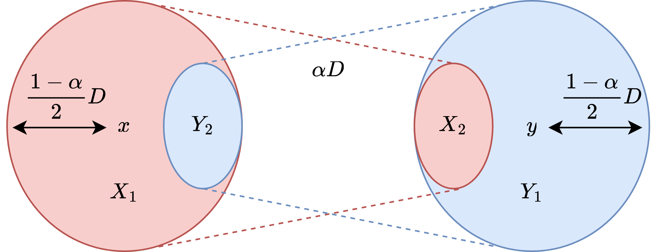
For a general approximation factor , instead of considering the red and the blue neighborhoods of a single point , consider a pair of points and take the red neighborhood of one and the blue neighborhood of the other. Define the red neighborhood of , and the blue neighborhood of , . Consider the points in that are within red distance of some point in , . Similarly, define . The sets are illustrated in figure 1, where distance is illustrated in red and distance is illustrated in blue.
As with the 3-approximation, these sets have two useful properties.
Claim 10.
If and then we can find a pair of points with .
Proof.
Take an arbitrary and . If , then
and so , a contradiction. Thus and similarly . Therefore .
Claim 11.
Let have distance . If and , then and .
Proof.
If , then and therefore . Thus, , in contradiction to . We arrive at a similar contradiction if .
Therefore, our goal is now to find a pair of points such that and . Using the above claims, this will allow us to find a pair of points with in linear time.
To do so, consider running BFS from an arbitrary point in both the red and the blue graphs . If the algorithm found no point such that , then is close to and in either red or blue. Since , we can assume without loss of generality that and . Now, if , since we assumed , there is some point on the shortest red path between and such that , and so
If then there exists a point on this shortest path such that and .
Similarly, there exists a point such that and . Therefore, by considering all pairs of points we can find a pair that satisfy the conditions of claim 11 and thus also the conditions of claim 10. Now, by running a linear time algorithm for every pair of points we can find a pair of points of distance . In fact, we don’t need to run the above algorithm for every pair of potential points independently. We can improve our running time using fast rectangular matrix multiplication. We use the standard notation to indicate the time it takes to multiply a matrix by a matrix using fast rectangular matrix multiplication.
We are now ready to claim the following generalization to our -approximation algorithm.
Lemma 12.
Let be a -multimode graph with -mode diameter . Given and a point with and , we can find a pair of points with in time .
Proof.
Define and . From every run BFS in to compute and as illustrated in figure 1 (without taking an intersection with ). Let be a matrix with rows indexed by and columns indexed by and let be a matrix with rows indexed by and columns indexed by . Define and as follows,
Similarly, run BFS from every in and define by,
Finally, compute the boolean matrix product
For any , we have and . Therefore, by claim 10, if we can find a pair of points with . If , there exist some for which and , and so by claim 11 at least one pair will have .
To summarize, in order to find a pair of points with we first run BFS from every point in and . We construct the matrices and use them to compute . We then find a pair such that . For this pair, we compute the sets and return and . These points satisfy . If we are unable to find such points we conclude that .
The final running time is dominated by for the BFS searches and to preform the matrix multiplications.
3.3 Linear Time -Approximation for -mode Diameter
In this section we consider a -multimode graph and attempt to approximate its -mode diameter. We extend our result for -multimode graphs and provide a near linear time -approximation algorithm for the -mode diameter.
To find a -approximation to the -mode diameter we will look for a pair of points with . We will use a similar approach to the 2-mode case, finding two sets in which all points are far apart in both the red and blue graphs (). We can then compute the ST-diameter of the two sets in green (), finding two points with large distance as well. As in previous sections, we provide an algorithm for unweighted graphs and note that by replacing BFS with Dijkstra’s algorithm the algorithm works for weighted graphs, while adding a factor to the running time.
Theorem 13.
Given a -multimode undirected, unweighted graph and integer , there exists an time algorithm that does one of the following with high probability:
-
1.
Finds a pair of points with .
-
2.
Determines that the 3-mode diameter of is .
By performing a binary search over the possible values of we obtain our desired result.
Proof.
Choose an arbitrary vertex and run BFS from it in all three graphs, . Let and . If there exists a vertex such that , then and so . We can therefore return and finish. Otherwise .
As was the case for 2-mode diameter, we note that for any pair of points , and so . Likewise, for any pair or we have and .
Thus, any pair of points within one of the sets has -mode distance . Next, consider pairs of points and . Run BFS in red from the set and run BFS in blue from the set . Let be the points in of red distance from the set . We claim that any pair of points have 3-mode distance . For any point there exists with . Therefore, .
Now define . Using a symmetric argument we can show every pair of points have distance . Therefore, if or , then every pair of points have distance .
Denote and . We are left to handle the case when both are non-empty. Every pair of points has and so in order to determine if we only need to consider .
To do so, preform a simple approximation to the ST-diameter of the sets in as follows. Pick two arbitrary nodes and run BFS from each one of them in . If then we will have found a point such that and so . Similarly, if , we will have found a point such that .
Otherwise, and . Thus, for every pair of points ,
And so we conclude that any pair of points have .
We can now repeat this algorithm for the pairs of sets and and their respective pairs of colors. If the algorithms finds no pair of points with , we conclude that the 3-mode diameter of is .
3.4 Linear Time 3-Approximation for -mode Radius
In the following section we consider the problem of approximating the -mode radius of a -multimode graph. Unlike the algorithms we constructed for approximating the -mode diameter, in this case we provide a general algorithm for all , with running time parameterized by and . Our algorithm provides a -approximation for the -mode radius and runs in time . Thus, for a constant we have a near linear time algorithm. We again present our algorithm for unweighted graphs and note that by replacing BFS with Dijkstra’s algorithm we can extend the result to weighted graphs while adding to the running time.
Theorem 14.
There exists an time algorithm that computes a -approximation of the -mode radius of an unweighted, undirected -multimode graph.
Proof.
Our algorithm receives a threshold and either finds a vertex with or determines that . Performing a binary search over the values of will give the desired approximation.
First we consider the 2-mode radius () and then we will show how to generalize this algorithm to any . Assuming , our approach will be to find a point that is close to the center of the graph in both colors. If we find a vertex with and , then for any vertex we have for some and so .
To find such a point, run BFS from an arbitrary node . If we are finished, otherwise we have a point with . The points are both within distance of the center in either red or blue, if were both within distance of the center in the same color we would have a contradiction. Thus, if , then me must have and if , then me must have .
Let and . By the above observation, is either in or in . If , then any point will have and . This would imply . Similarly, if then any point will have . Therefore, by choosing arbitrary and running BFS from each, we will have found a vertex of eccentricity .
This algorithm runs a constant number of BFSs and if it finds a point with . Otherwise, we can conclude . Therefore, in time our algorithm provides a -approximation the the -mode radius. We can now extend this idea to any value of .
For a general we can define a recursive algorithm, where at each node we “guess” the color (or mode) in which it achieves its distance to the center (in fact we try all possible colors). We run algorithm 1, , on input , a subset of colors and a subset of vertices . We would like to have the following property:
-
(P1)
If , then and for .
Correctness.
We run algorithm 1 on and at first, at which point (P1) trivially holds. Subsequently, we claim that if satisfy (P1), then in at least one of the recursive calls in line 9, the sets satisfy (P1).
Let and be such that (as chosen in lines 3,6). Since for any , we must have . Thus, there exists such that . For this iteration of the for the loop in line 7, we have and so any point has . Hence satisfy property (P1).
Therefore, there exists at least one path of length in the recursion tree for which (P1) is maintained at all levels of the recursion. Since each call adds a color to , after calls we will have . In this case, is a nonempty set which has for any . Thus, any will have and will be returned in line 4. If no is returned by the algorithm we can conclude that .
Runtime.
Every call to preforms a constant number of BFS searches and calls to with . Therefore, the total running time of the algorithm is .
References
- [1] Amir Abboud, Virginia Vassilevska Williams, and Joshua Wang. Approximation and fixed parameter subquadratic algorithms for radius and diameter in sparse graphs. In Proceedings of the Twenty-Seventh Annual ACM-SIAM Symposium on Discrete Algorithms, SODA ’16, pages 377–391, USA, 2016. Society for Industrial and Applied Mathematics. doi:10.1137/1.9781611974331.CH28.
- [2] Arturs Backurs, Liam Roditty, Gilad Segal, Virginia Vassilevska Williams, and Nicole Wein. Toward tight approximation bounds for graph diameter and eccentricities. SIAM Journal on Computing, 50(4):1155–1199, 2021. doi:10.1137/18M1226737.
- [3] Aaron Berger, Jenny Kaufmann, and Virginia Vassilevska Williams. Approximating Min-Diameter: Standard and Bichromatic. In Inge Li Gørtz, Martin Farach-Colton, Simon J. Puglisi, and Grzegorz Herman, editors, 31st Annual European Symposium on Algorithms (ESA 2023), volume 274 of Leibniz International Proceedings in Informatics (LIPIcs), pages 17:1–17:14, Dagstuhl, Germany, 2023. Schloss Dagstuhl – Leibniz-Zentrum für Informatik. doi:10.4230/LIPIcs.ESA.2023.17.
- [4] Massimo Cairo, Roberto Grossi, and Romeo Rizzi. New bounds for approximating extremal distances in undirected graphs. In Robert Krauthgamer, editor, Proceedings of the Twenty-Seventh Annual ACM-SIAM Symposium on Discrete Algorithms, SODA 2016, Arlington, VA, USA, January 10-12, 2016, pages 363–376. SIAM, 2016. doi:10.1137/1.9781611974331.CH27.
- [5] Chris Calabro, Russell Impagliazzo, and Ramamohan Paturi. On the exact complexity of evaluating quantified k-cnf. In Venkatesh Raman and Saket Saurabh, editors, Parameterized and Exact Computation - 5th International Symposium, IPEC 2010, Chennai, India, December 13-15, 2010. Proceedings, volume 6478 of Lecture Notes in Computer Science, pages 50–59. Springer, 2010. doi:10.1007/978-3-642-17493-3_7.
- [6] Shiri Chechik, Daniel H. Larkin, Liam Roditty, Grant Schoenebeck, Robert Endre Tarjan, and Virginia Vassilevska Williams. Better approximation algorithms for the graph diameter. In Chandra Chekuri, editor, Proceedings of the Twenty-Fifth Annual ACM-SIAM Symposium on Discrete Algorithms, SODA 2014, Portland, Oregon, USA, January 5-7, 2014, pages 1041–1052. SIAM, 2014. doi:10.1137/1.9781611973402.78.
- [7] Shiri Chechik and Tianyi Zhang. Constant approximation of min-distances in near-linear time. In 2022 IEEE 63rd Annual Symposium on Foundations of Computer Science (FOCS), pages 896–906. IEEE, 2022. doi:10.1109/FOCS54457.2022.00089.
- [8] Lenore Cowen and Christopher G. Wagner. Compact roundtrip routing for digraphs. In Robert Endre Tarjan and Tandy J. Warnow, editors, Proceedings of the Tenth Annual ACM-SIAM Symposium on Discrete Algorithms, 17-19 January 1999, Baltimore, Maryland, USA, pages 885–886. ACM/SIAM, 1999. URL: http://dl.acm.org/citation.cfm?id=314500.315068.
- [9] Mina Dalirrooyfard and Jenny Kaufmann. Approximation Algorithms for Min-Distance Problems in DAGs. In Nikhil Bansal, Emanuela Merelli, and James Worrell, editors, 48th International Colloquium on Automata, Languages, and Programming (ICALP 2021), volume 198 of Leibniz International Proceedings in Informatics (LIPIcs), pages 60:1–60:17, Dagstuhl, Germany, 2021. Schloss Dagstuhl – Leibniz-Zentrum für Informatik. doi:10.4230/LIPIcs.ICALP.2021.60.
- [10] Mina Dalirrooyfard, Ray Li, and Virginia Vassilevska Williams. Hardness of approximate diameter: Now for undirected graphs. In 62nd IEEE Annual Symposium on Foundations of Computer Science, FOCS 2021, Denver, CO, USA, February 7-10, 2022, pages 1021–1032. IEEE, 2021. doi:10.1109/FOCS52979.2021.00102.
- [11] Mina Dalirrooyfard, Virginia Vassilevska Williams, Nikhil Vyas, and Nicole Wein. Tight approximation algorithms for bichromatic graph diameter and related problems. In Christel Baier, Ioannis Chatzigiannakis, Paola Flocchini, and Stefano Leonardi, editors, 46th International Colloquium on Automata, Languages, and Programming, ICALP 2019, July 9-12, 2019, Patras, Greece, volume 132 of LIPIcs, pages 47:1–47:15. Schloss Dagstuhl – Leibniz-Zentrum für Informatik, 2019. doi:10.4230/LIPICS.ICALP.2019.47.
- [12] Mina Dalirrooyfard, Virginia Vassilevska Williams, Nikhil Vyas, Nicole Wein, Yinzhan Xu, and Yuancheng Yu. Approximation Algorithms for Min-Distance Problems. In Christel Baier, Ioannis Chatzigiannakis, Paola Flocchini, and Stefano Leonardi, editors, 46th International Colloquium on Automata, Languages, and Programming (ICALP 2019), volume 132 of Leibniz International Proceedings in Informatics (LIPIcs), pages 46:1–46:14, Dagstuhl, Germany, 2019. Schloss Dagstuhl – Leibniz-Zentrum für Informatik. doi:10.4230/LIPIcs.ICALP.2019.46.
- [13] Mina Dalirrooyfard and Nicole Wein. Tight conditional lower bounds for approximating diameter in directed graphs. In Samir Khuller and Virginia Vassilevska Williams, editors, STOC ’21: 53rd Annual ACM SIGACT Symposium on Theory of Computing, Virtual Event, Italy, June 21-25, 2021, pages 1697–1710. ACM, 2021. doi:10.1145/3406325.3451130.
- [14] Russell Impagliazzo and Ramamohan Paturi. On the complexity of k-sat. Journal of Computer and System Sciences, 62(2):367–375, 2001. doi:10.1006/jcss.2000.1727.
- [15] Lung-Hao Lee and Yi Lu. Multiple embeddings enhanced multi-graph neural networks for chinese healthcare named entity recognition. IEEE Journal of Biomedical and Health Informatics, 25(7):2801–2810, 2021. doi:10.1109/JBHI.2020.3048700.
- [16] Liam Roditty and Virginia Vassilevska Williams. Fast approximation algorithms for the diameter and radius of sparse graphs. In Dan Boneh, Tim Roughgarden, and Joan Feigenbaum, editors, Symposium on Theory of Computing Conference, STOC’13, Palo Alto, CA, USA, June 1-4, 2013, pages 515–524. ACM, 2013. doi:10.1145/2488608.2488673.
- [17] Liam Roditty and Uri Zwick. On dynamic shortest paths problems. In Algorithms–ESA 2004: 12th Annual European Symposium, Bergen, Norway, September 14-17, 2004. Proceedings 12, pages 580–591. Springer, 2004. doi:10.1007/978-3-540-30140-0_52.
- [18] Fei Tian, Hanjun Dai, Jiang Bian, Bin Gao, Rui Zhang, Enhong Chen, and Tie-Yan Liu. A probabilistic model for learning multi-prototype word embeddings. In Proceedings of COLING 2014, the 25th International Conference on Computational Linguistics: Technical Papers, pages 151–160, 2014. URL: https://aclanthology.org/C14-1016/.
- [19] Virginia Vassilevska Williams. On some fine-grained questions in algorithms and complexity. In Proceedings of the ICM, volume 3, pages 3431–3472. World Scientific, 2018.
- [20] Zixuan Xu Virginia Vassilevska Williams, Yinzhan Xu and Refei Zhou. New bounds for matrix multiplication: from alpha to omega. In Proceedings of the 2024 Annual ACM-SIAM Symposium on Discrete Algorithms (SODA), pages 3792–3835, 2024. doi:10.1137/1.9781611977912.134.
- [21] Canwen Xu, Feiyang Wang, Jialong Han, and Chenliang Li. Exploiting multiple embeddings for chinese named entity recognition. In Proceedings of the 28th ACM International Conference on Information and Knowledge Management, CIKM ’19, pages 2269–2272, New York, NY, USA, 2019. Association for Computing Machinery. doi:10.1145/3357384.3358117.