Leveraging Open-Source Satellite-Derived Building Footprints for Height Inference

Abstract
At a global scale, cities are growing and characterizing the built environment is essential for deeper understanding of human population patterns, urban development, energy usage, climate change impacts, among others. Buildings are a key component of the built environment and significant progress has been made in recent years to scale building footprint extractions from satellite datum and other remotely sensed products. Billions of building footprints have recently been released by companies such as Microsoft and Google at a global scale. However, research has shown that depending on the methods leveraged to produce a footprint dataset, discrepancies can arise in both the number and shape of footprints produced. Therefore, each footprint dataset should be examined and used on a case-by-case study. In this work, we find through two experiments on Oak Ridge National Laboratory and Microsoft footprints within the same geographic extent that our approach of inferring height from footprint morphology features is source agnostic. Regardless of the differences associated with the methods used to produce a building footprint dataset, our approach of inferring height was able to overcome these discrepancies between the products and generalize, as evidenced by 98% of our results being within of the ground-truthed height. This signifies that our approach can be applied to the billions of open-source footprints which are freely available to infer height, a key building metric. This work impacts the broader domain of urban science in which building height is a key, and limiting factor.
Keywords and phrases:
Building Height, Big Data, Machine LearningCopyright and License:
2012 ACM Subject Classification:
Computing methodologies Machine learning ; Computing methodologies Classification and regression trees ; Computing methodologies Neural networks ; Applied computingAcknowledgements:
Notice: This manuscript has been authored by UT-Battelle, LLC, under contract DE-AC05-00OR22725 with the US Department of Energy (DOE). The US government retains a nonexclusive, paid-up, irrevocable, worldwide license to publish or reproduce the published form of this manuscript, or allow others to do so, for US government purposes. DOE will provide public access to these results of federally sponsored research in accordance with the DOE Public Access Plan (http://energy.gov/downloads/doe-public-access-plan).Editors:
Katarzyna Sila-Nowicka, Antoni Moore, David O'Sullivan, Benjamin Adams, and Mark GaheganSeries and Publisher:
1 Introduction
Populations are increasing at a global scale, and it is estimated that by 2050, 68% of the global population will live in urban environments [17, 20]. Buildings are a key component of the urban environment and their footprints have been used across a myriad of subjects such as population density estimation [31, 32], building energy usage [12, 39], disaster management [28], building type [1], building height [6, 25, 37] and urban heat islands (UHI’s) [10]. Being able to characterize the built environment is imperative to address these issues and information on building footprints, building height and urban morphology is critical in these efforts.
Fortunately, over the past decade, there has been a dramatic increase in the amount of open-source building footprint datum available from organizations such as Microsoft222https://www.microsoft.com/en-us/maps/bing-maps/building-footprints, Google333https://sites.research.google/open-buildings/, and Oak Ridge National Laboratory (ORNL)444https://gis-fema.hub.arcgis.com/pages/usa-structures. Between these products, there are over 3 billion footprints available for use. However, each of the aforementioned products is generated via differing methods for the pixel extraction/segmentation to identify buildings and the regularization process of the identified footprints. Furthermore, differences in imagery sources and resolution as well as environmental factors such as shadows or sun angle can also influence the footprint extraction and regularization process [13].
The processing workflow from Microsoft is described in their documentation as first leveraging a deep neural network (DNN) to identify buildings from aerial imagery and then converting the identified pixels into polygons representing building footprints555https://github.com/microsoft/GlobalMLBuildingFootprints. The best available information on Google’s footprint generation is from a paper in 2023 by Sirko et al. [35]. In their report, the authors describe utilizing a U-Net model, a common approach for segmenting satellite datum [2, 29, 38]. Once extracted, the building footprints are then processed through a contouring algorithm that realigns groups of adjacent polygons to regularize the building footprints [35]. The authors also provide a caveat that newer versions (v2 and v3) of the Google Open Buildings dataset underwent further improvements that are not documented. Of the three datasets, ORNL provides the highest level of detail in how building footprints were both extracted and regularized from satellite datum as they leverage a deep convolutional neural network (CNN) framework for pixel extraction and the ArcGIS proprietary building footprint regularization module 666https://pro.arcgis.com/en/pro-app/latest/tool-reference/3d-analyst/regularize-building-footprint.htm [41, 42]. However, the ORNL footprint dataset is only available publicly in the United States (U.S.), so it lacks the volume and spatial scale of building footprints that Microsoft and Google provide. While Microsoft, Google, and ORNL each utilize a deep learning framework to identify, delineate, and regularize the footprints, there are proven differences associated with the footprints provided by each entity [8, 14].
Chamberlain et al. found substantial differences between footprint patterns displayed by Microsoft and Google when comparing the products at a grid scale in Africa [8]. The authors noted that consideration is needed by users regarding the suitability of the specific building footprint dataset for its intended application. For example, in urban areas, Microsoft seemed to have better coverage in relation to the number of matching footprints, but this pattern was not universal. Also in Africa, Gonzales found patterns of irregularity when comparing Google and Microsoft, but at a building-by-building level [14]. When investigating urban areas, Microsoft tended to generate larger footprints which may encapsulate multiple buildings while Google seemed to have more, smaller buildings. When rural areas were investigated, the building counts were relatively similar, showing little discrepancy. Both at scale and at a building-by-building level, care must be taken when leveraging footprint datasets [8, 14].
Recently, research has shown that building height is obtainable based on building footprint information alone [37]. The authors showcased a novel method to infer height at a high accuracy using only information derived from an individual buildings footprint. Furthermore, they did so based on footprints extracted from both lidar and satellite datum. The ability to infer height from footprints extracted from satellite datum allows for this approach to generate building height maps at large scale. However, the authors only demonstrated their approach on building footprints developed by ORNL and the model inference may produce irregular results when exposed to a different footprint source. For example, in Stipek et. al [37] they discuss that the features with the highest impact on inferring building height were contextual (number of neighbors) and engineered (complexity of footprint shape). It has been proven that at both a grid [8] and building-by-building level [14], Microsoft and Google have differing shapes and sizes which would affect the contextual and engineered metrics generated at the building level. Therefore, it would be imprudent to assume the approach proposed by Stipek et al. [37] can be applied to other footprint datasets without further testing.
In this paper we demonstrate that it is possible to infer building height at a building-by-building level, agnostic to footprint source. We prove this by comparing the inferred heights from two distinct products, ORNL and Microsoft across 10 cities in the U.S., with figure 1 showcasing the spatial extent of our research. We show that regardless of differences associated with the extraction, regularization of the footprints and other factors, such as imagery date or environmental factors, our approach of inferring height from footprints can be applied to ORNL and Microsoft footprints. This signifies that it is possible to leverage the 1.2 billion footprints which Microsoft has made openly available to infer height at a global scale. Google footprints are not currently available in the U.S. and this research only focused on ORNL and Microsoft footprints.

2 Related Works
While the authors acknowledge a deep field of literature in relation to leveraging deep learning on satellite datum, we would like to bring attention to works which relate to extracting building information. Secondly, we focus on studies that have inferred height from features derived from building footprints.
2.1 Footprint Extraction and Regularization
There have been various methods to segment and regularize footprints derived from high-resolution satellite datum [4, 9, 23, 26, 30, 34, 35, 36, 40, 42, 43]. Shi et al. leverage a large-scale deep learning mapping framework using Google Earth images to map 280 million building footprints in east Asia [34]. They note in their work that existing building extraction models primarily utilize supervised deep learning methods which lack generalization due to differences in building morphologies. For example, buildings in east Asia are more compact and display more diverse patterns as compared to buildings within the U.S. or Europe. The authors further discuss the issues associated with the regularization of the identified buildings, stating that building footprints differ based on the methods leveraged. To address for this, after the footprints are extracted from the satellite datum, they deploy a stable boundary optimization algorithm which uses a generative adversarial learning network (GAN) to enhance the semantic features of buildings. To regularize the footprints, they used a post-processing method proposed by Gribov [16].
Sirko et al., in developing Google’s Open Buildings dataset, leveraged a U-Net architecture, a deep learning encoder-decoder model for semantic segmentation for pixel identification from imagery [33, 35]. This approach classifies each pixel of an image as either a building or a non-building. They tested this approach using a training set of 99,902 satellite images across the African continent and note that two of the more complex issues they faced were smaller buildings, and buildings in densely populated areas. To address for this, they taught their model to predict at least one pixel gap between the buildings, which they accomplished by employing a morphological erosion operation with a kernel size of 3x3 pixels during pre-processing. Once footprints were identified and pre-processed, they then deployed a contouring algorithm to produce angular shapes and realign groups of nearby polygons.
For the development of the ORNL building footprint dataset, Yang et al. developed a CNN framework to extract pixels which represented structures [41, 42]. Furthermore, the authors also incorporated custom designed signed-distance labels which aided in improving the building outline extraction which was especially helpful in core urban areas where there are high densities of buildings within a small area. Once footprints were identified, they leveraged the ArcGIS building footprint regularization module. Using this approach, the authors provided a simple and effective method that successfully produced a building footprint map of the U.S.
2.2 Building Height - Machine Learning Approach from Morphology Features
In 2017, Biljecki et al. leveraged a random forest model to infer building height from footprint and ancillary information, such as number of floors [6]. The authors tested their approach on 200,000 buildings in the Netherlands and found that it is possible to infer height using a tree-based approach. However, some of the features used, such as number of floors, are a proxy for height and this metric is not available at scale, thus limiting the scalability of their approach. Furthermore, their analysis was done on footprints extracted from lidar datum, thus further hindering them to areas in which lidar footprints are available.
Milojevic-Dupont built upon this work and leveraged a gradient boosting algorithm, XGBoost, to infer height for buildings in Europe (Germany, Netherlands, France, Italy) [25]. They expanded the morphology features derived from building footprints compared to Biljecki [6], and also used ancillary datasets, such as road networks, with a total of 152 features used in their modeling approach. However, similar to the approach by Biljecki, they utilized footprints derived from lidar datum, thus suffering from the same constraint of limited scalability at a continental or global scale.
Stipek et al. expanded upon the work done by the previous authors and inferred height from building footprints without the use of ancillary information [37]. The authors leveraged morphology features generated from individual buildings and successfully inferred height on both lidar-derived and satellite-derived building footprints. However, they only showcased their ability to infer height on ORNL footprints, thus limiting their approach to that singular dataset.
3 Methods
Here, we discuss the methodology used for our research which aims to address if it is possible to infer height based on footprints derived from satellite datum which have been identified and regularized using varying methods. For this work we leverage 3.09 million building records across the U.S. (Table 1). We selected 10 cities within the U.S. that had satellite derived footprints from ORNL and Microsoft which overlapped with lidar derived footprints, which had a height associated with the footprints (Figure 1).
3.1 Footprint Datasets
3.1.1 ORNL Footprints
This dataset contains footprints for the cities of Albany, Boise, Boston, Houston, Nashville, Omaha, Phoenix, Portland, Seattle, and Topeka within the U.S. The footprints are derived from satellite datum based on the approach in Yang et al. [42]. Please note that the current version of footprints within the USA Structures dataset are lidar generated footprints after replacement for the reasons described by Yang et al. [41]. However, we chose to use the earlier version of the satellite derived footprints for fair comparison.
3.1.2 Microsoft Footprints
The Microsoft dataset provides over 1 billion footprints spanning multiple continents777https://www.microsoft.com/en-us/maps/bing-maps/building-footprints. These building footprints were developed from a deep learning model which extracted pixel information from satellite datum. The pixels, once identified as a building, then underwent a thorough cleaning and regularization process. Microsoft has multiple releases for their building footprint dataset and we leverage the footprints Microsoft released on 26/04/2023 for the 10 cities within the U.S. (Table S1).
3.1.3 Lidar Footprints
The lidar footprints leveraged in this research are publicly available as part of the USA Structures dataset at the FEMA portal888https://gisfema.hub.arcgis.com/pages/usa-structures [41].
| Microsoft | ||||||||||
| Metric | Albany | Boise | Boston | Houston | Nashville | Omaha | Phoenix | Portland | Seattle | Topeka |
| Count | 108,107 | 64,935 | 177,997 | 215,552 | 50,115 | 162,180 | 469,485 | 104,307 | 40,169 | 49,739 |
| Mean | 5.50 m | 4.16 m | 6.94 m | 4.28 m | 4.63 m | 4.96 m | 3.85 m | 4.86 m | 5.05 m | 4.39 m |
| Median | 5.33 m | 3.83 m | 6.89 m | 3.74 m | 4.27 m | 4.77 m | 3.48 m | 4.47 m | 4.53 m | 4.09 m |
| Std | 1.54 m | 1.24 m | 1.95 m | 1.72 m | 1.52 m | 1.30 m | 1.24 m | 1.71 m | 2.39 m | 1.26 m |
| 25% | 4.41 m | 3.34 m | 5.61 m | 3.40 m | 3.74 m | 4.14 m | 3.15 m | 3.68 m | 3.77 m | 3.59 m |
| 75% | 6.33 m | 4.75 m | 8.04 m | 4.65 m | 5.09 m | 5.55 m | 4.17 m | 5.64 m | 5.71 m | 4.89 m |
| Max | 41.16 m | 60.77 m | 72.69 m | 180.90 m | 71.22 m | 78.32 m | 77.07 m | 69.71 m | 146.45 m | 46.32 m |
| ORNL | ||||||||||
| Count | 116,518 | 74,901 | 198,631 | 261,225 | 59,597 | 181,672 | 522,666 | 122,048 | 51,219 | 56,038 |
| Mean | 5.54 m | 4.16 m | 7.01 m | 4.32 m | 4.60 m | 4.95 m | 3.86 m | 4.88 m | 5.09 m | 4.37 m |
| Median | 5.35 m | 3.83 m | 6.95 m | 3.75 m | 4.25 m | 4.76 m | 3.48 m | 4.48 m | 4.56 m | 4.07 m |
| Std | 1.61 m | 1.25 m | 2.01 m | 1.82 m | 1.51 m | 1.34 m | 1.27 m | 1.72 m | 2.45 m | 1.27 m |
| 25% | 4.42 m | 3.34 m | 5.66 m | 3.39 m | 3.73 m | 4.12 m | 3.14 m | 3.69 m | 3.77 m | 3.58 m |
| 75% | 6.39 m | 4.76 m | 8.14 m | 4.70 m | 5.05 m | 5.55 m | 4.18 m | 5.65 m | 5.80 m | 4.88 m |
| Max | 71.00 m | 60.77 m | 101.82 m | 180.90 m | 71.22 m | 78.32 m | 96.90 m | 69.71 m | 146.45 m | 46.32 m |
Descriptive statistics for the cities selected in this research with Microsoft buildings on the top panel and ORNL footprints on the bottom panel. Please note the differing number of total buildings based on the one-to-one conflation method. For example, the count of buildings in Albany is 108,107 for Microsoft with 116,518 for ORNL.
3.2 Lidar Conflation
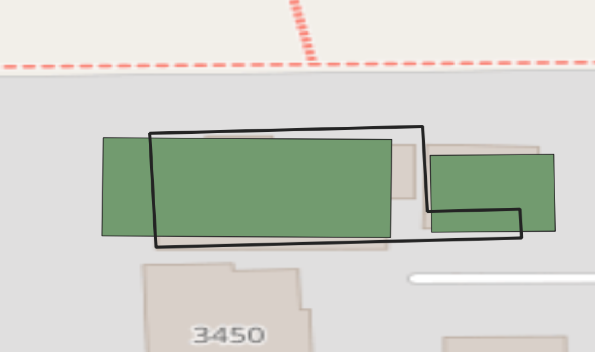
We followed the same conflation approach as proposed by Stipek et al. [37]. Conflating two datasets collected at differing temporal scales can prove to be problematic due to periods of growth exhibited by the area-of-interest. Therefore, we followed a strict one-to-one relationship requirement when conflating the lidar footprints to both the Microsoft and ORNL footprint datasets (Fig. 2). Please note this conflation process ended with a different number of matched footprints. For example, in Albany, the matching one-to-one footprints for lidar to Microsoft were 108,107 and 116,518 for ORNL (Table 1).


3.3 Morphology Features
We utilized morphology features generated from vector geospatial polygon layers at a building-by-building level [18]. Morphology features have been leveraged to infer building use type, building height, among others [1, 6, 25, 37]. The morphology feature set consists of three types of features: geometric, engineered, and contextual (Table S2). Geometric are basic measures of geometry like area or perimeter. Engineered features describe more complex ideas like compactness or complexity. Contextual features describe the building and its relationship to its neighbors, both spatially and in size. The contextual features are generated at five different scales: , , , , and . Overall, there are 65 features generated with table S2 providing a description of each feature. The morphology feature set was generated for the ORNL and Microsoft footprints which were selected during the conflation process. We also compared the morphology features generated for each of the 10 cities between the ORNL and Microsoft footprints to better understand the differences between the two footprint datasets.
3.4 Feature Selection
All buildings less than in height were removed from both datasets, a common practice when inferring height from 2D features [25, 37]. Feature reduction was then performed for both datasets via a recursive feature elimination (RFE). This iterative function removes features that display lower significance in relation to the target variable [15]. The features selected for by the RFE are bolded in table S2.
3.5 Model Development
We applied 4 distinct models during this research and compared to a baseline metric, the median, over which any model would be an improvement. The first model we applied, a Linear Regression (LR) model provides a baseline initial estimate and works by assuming there is a linear relationship between the target, height, and the training datum [19]. We next applied a Random Forest (RF) algorithm, first introduced by Breiman [7]. The RF model is a collection of tree-structured classifiers with each tree within a defined forest coming to a decision independent of the other trees. After each tree has inferred a decision based on a random subset of the training datum, a decision is then made for inferrence based on a majority vote from the individual trees. The XGBoost Regressor (XGB) is a gradient boosting trees algorithm in which decision trees are iteratively added and learn from the previous tree in order to minimize error[11]. This allows for the XGB to learn from each successive tree such that the model will reduce error and improve overall model performance. TabNet, a novel high-performance deep learner designed to help improve tabular datum predictions was also applied [3]. TabNet has been shown to improve run-time and display comparable results to other gradient boosting algorithms [22]. This is the first time, to the authors knowledge, that a deep learning framework has been applied to infer building height from tabular datum. Each model was constructed for each of the cities for both the Microsoft and ORNL footprint datasets and the ensuing steps were taken for each city within both datasets, totalling 20 iterations.
Each city was split into a training and testing dataset, with 70% used for training and 30% for testing. We then leveraged Bayesian optimization using the Hyperopt library [5]. The Bayesian optimization utilizes a prior set of hyper-parameters to inform the successive set of hyper-parameters for testing. It iterates through this process and once complete, it produces the optimum hyper-parameters from a pre-defined grid search space in relation to the lowest RMSE. We selected the following hyper-parameters to fine-tune through the Bayesian optimization: number of estimators, max depth, gamma, reg alpha, reg lambda, colsample bytree, min child weight, and learning rate. To validate our results, we conducted a 10 fold cross validation (CV) over the entirity of the datum for each individual city. Please note that all references to the XGB RMSE are in reference to the CV score.
3.6 Out of Sample Validation
While conducting a 10-fold CV, we acknowledge that when working with spatially diverse datum, validation should also be applied to distinct geographic areas [24]. To account for this, we conducted a spatial validation similar to that done by Metzger et al. [24] and Stipek et al. [37] in which we randomly selected 3 cities (Albany, Houston, Seattle) as hold-out validation cities for testing for both datasets (ORNL, Microsoft) (Figure S1).
4 Results
The XGB model was chosen based on its superior performance in relation to the other models applied (LR, RF, TabNet). While we acknowledge that the RF outperformed the XGB in certain cities, the XGB was more consistent across both datasets (ORNL, Microsoft). All the results in the following sections are the inferred values from the XGB model. For the results associated with the LR, RF, and TabNet models please see Supplementary Table S3.
4.1 Microsoft Footprints
Each of the 10 cities modeled within the Microsoft dataset showed improvement upon the median value generated for both the MAE and RMSE (Table 2). The median values generated present a baseline value for building height over which any improvement in relation to MAE or RMSE can be considered an improvement over a baseline estimate. Phoenix showed the highest goodness of fit, , with a metric of 61% with Nashville displaying the lowest, 39%. In relation to improvement upon the median RMSE baseline, Seattle was the highest, with improvement, going from the median of to a modeled output RMSE of . Topeka and Albany displayed the lowest improvement, displaying differences of and , respectively. On average, the percentage improvement across the 10 cities from the median RMSE to the modeled RMSE was 32%.
| Microsoft | ||||||||||
| Metric | Albany | Boise | Boston | Houston | Nashville | Omaha | Phoenix | Portland | Seattle | Topeka |
| Median MAE | 1.12 m | 0.84 m | 1.45 m | 0.92 m | 0.91 m | 0.91 m | 0.78 m | 1.15 m | 1.30 m | 0.82 m |
| Median RMSE | 1.55 m | 1.28 m | 1.95 m | 1.80 m | 1.56 m | 1.32 m | 1.30 m | 1.75 m | 2.44 m | 1.29 m |
| XGBoost MAE | 0.82 m | 0.58 m | 1.00 m | 0.64 m | 0.69 m | 0.60 m | 0.45 m | 0.82 m | 1.01 m | 0.58 m |
| XGBoost RMSE | 1.20 m | 0.89 m | 1.47 m | 1.21 m | 1.17 m | 0.95 m | 0.80 m | 1.27 m | 1.85 m | 1.00 m |
| XGBoost | 40% | 46% | 45% | 48% | 39% | 51% | 61% | 48% | 42% | 41% |
| % Improvement | 25% | 36% | 28% | 39% | 29% | 33% | 48% | 32% | 28% | 25% |
| ORNL | ||||||||||
| Median MAE | 1.15 m | 0.85 m | 1.48 m | 0.96 m | 0.90 m | 0.91 m | 0.79 m | 1.16 m | 1.33 m | 0.82 m |
| Median RMSE | 1.63 m | 1.30 m | 2.02 m | 1.90 m | 1.55 m | 1.35 m | 1.33 m | 1.77 m | 2.49 m | 1.31 m |
| XGBoost MAE | 0.85 m | 0.61 m | 1.03 m | 0.68 m | 0.72 m | 0.63 m | 0.49 m | 0.86 m | 1.02 m | 0.60 m |
| XGBoost RMSE | 1.26 m | 0.91 m | 1.49 m | 1.33 m | 1.24 m | 0.98 m | 0.81 m | 1.30 m | 1.91 m | 1.01 m |
| XGBoost | 39% | 44% | 43% | 46% | 41% | 47% | 60% | 42% | 38% | 40% |
| % Improvement | 26% | 35% | 30% | 35% | 22% | 32% | 49% | 31% | 26% | 26% |
Please note that the top panel are model results from the Microsoft footprints with the model results derived from ORNL footprints on the bottom panel. For the metrics, we display the MAE and RMSE associated with the median before displaying the model (XGBoost) results below. The median results are the baseline over which any model is an improvement over the simplest possible method in relation to inferring building height. We also display the % difference between the CV RMSE and median RMSE to showcase the improvement upon the baseline.
4.2 ORNL Footprints
The modeled ORNL footprints also showed improvement upon the median MAE and RMSE for each of the 10 cities (Table 2). Phoenix displayed the highest score, 60%, with Seattle displaying the lowest, with a score of 38%. For improvement upon the RMSE baseline, Seattle showed the highest improvement, , with Topeka displaying the lowest, . The average percent improvement from the median RMSE to the modeled RMSE across the 10 cities was 31%.
Across all 10 cities, the largest difference between the Microsoft and ORNL footprints in relation to RMSE was , observed in both Albany and Nashville with the lowest difference observed being in Topeka. In relation to the percentage improvement upon the median baseline for RMSE when comparing Microsoft and ORNL, the largest difference in improvement was 7% (29% - Microsoft, 22% - ORNL), observed in Nashville with six of the cities showing only 1% difference.
4.3 Morphology Differences
When comparing the differences between the morphology features generated for the ORNL and Microsoft footprints, the majority of the features showed minimal differences. However, there were some features which displayed differences, primarily the contextual and engineered features such as complexity ps, n count, and n size mean (Table S4). For the Microsoft footprints, the complexity ps displayed a median of 2,812 while the ORNL median was 7,717, signifying differences within the shapes of the footprints (Table S4). For the n count 500, Microsoft displayed a max count of 1,267, compared to 928 for ORNL, signifying a difference in the number of footprints within a radius. For n size mean 500, the max feature displayed by Microsoft was 210,048 with a value of 102,230 by ORNL, highlighting the differences in footprint sizes within a radius. These results are similar to the research conducted by Chamberlain et al. ([8]) and Gonzales ([14]).
4.4 Out of Sample Validation
When testing on Microsoft footprints, Albany did not improve upon the median RMSE as the XGB RMSE displayed a value of and a score of -1% (Table S5). However, the other cities which were tested with Microsoft footprints showed improvements upon the median RMSE, being in Houston and in Seattle. All three of the cities when tested on ORNL footprints displayed improvements upon the median RMSE, being for Albany, for Houston and for Seattle.
5 Discussion
The expansion of open-source building footprint datasets has provided the possibility for leveraging these products to characterize the built environment. Our results show that, across 3.09 million buildings in the U.S., our method of inferring height from footprint information alone is effective for datasets produced by ORNL as well as the much larger and globally available dataset from Microsoft. Furthermore, our height prediction process is reliable and agnostic to building footprint source. This finding ensures that our approach of inferring height from footprint morphology features can be scaled to leverage other publicly available footprints, such as Microsoft footprints. By inferring building height, this method provides valuable contextual information for population density estimation, building energy, disaster management, and UHI’s [10, 12, 31, 32, 39].


While the main objective of this research is to test the efficacy of leveraging open-source footprints, we applied various models to ensure the best possible method was selected. It is important to note that the TabNet model did not outperform either the RF or XGB for any cities across both footprint sources. In some instances, such as in Phoenix, the difference was -18% in relation to results displayed by the XGB. However, in other cities (Houston), the TabNet outperformed the percent improvement displayed by the RF by +1% in relation to . Regardless, the tree based approach consistently outperformed the TabNet model which signifies that while deep learning models developed for tabular data have made progress [21, 22], in this instance tree based models show higher accuracy.
While successful, our study does have limitations that need to be acknowledged. First, the area-of-interest is only within one country, the U.S., and more work is needed to expand this approach to additional countries. It is known that the built environment varies both spatially and temporally and a more diverse sample set is needed to further validate this approach [6, 25, 27, 34, 37]. Another limitation is that during our strict one-to-one conflation process, building footprints that don’t have a one-to-one match are removed and therefore not included in the morphology feature generation. Contextual features that look at a building’s neighbors have been found to be influential to the model’s behaviour and therefore, the model may not perform as well on the filtered dataset as it would on the unfiltered dataset [37]. For example, the generated feature n count measures the number of centroids within a defined radius surrounding a building. This was evidenced by the range of values displayed for the n count 500 for the ORNL when compared to Microsoft (Table S4). The range in values for n count 500 signifies that at a 500 m radius, there are differences associated with the total number of buildings, which can influence the model’s ability to infer an individual building’s height.
Additionally, there needs to be a formal analysis completed to understand if it is possible to train on one distinct footprint dataset and test on another. For example, due to the differences discussed between the Google and Microsoft datasets within Africa [8, 14], can it be possible to train on the Google footprints to then infer height on the Microsoft footprints. While the approach presented in this research shows the ability to infer height agnostic of footprint source, it does not test across the sources, i.e. training on ORNL and testing on Microsoft.
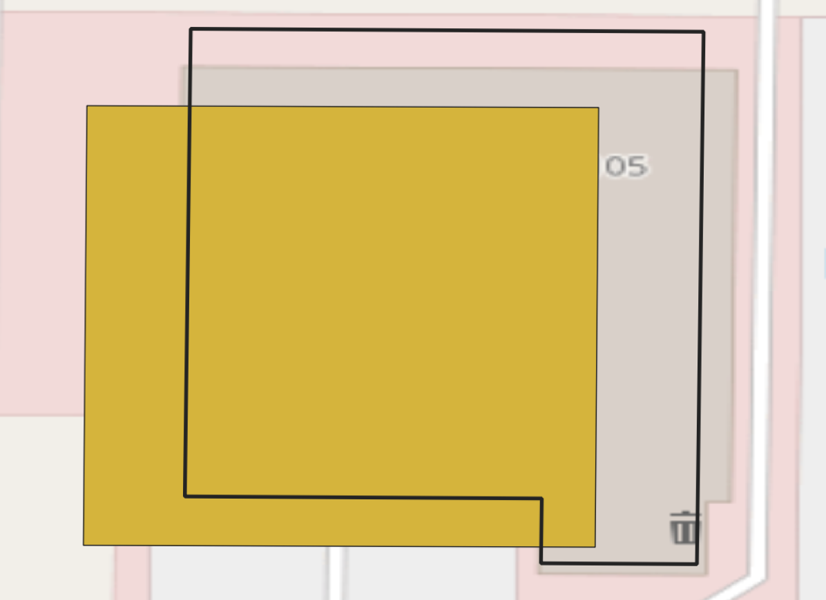
Furthermore, the differences in footprint shape based on the pixel identification and regularization process can lead to irregularities in predicted height (Fig. 3). For example, the complexity ratio, an engineered feature that is the shape length divided by the shape area which shows high significance in relation to inferring height, can vary depending on the footprint shape [37]. For example, in Boston, we display the Microsoft, ORNL and lidar footprint for one specific building where the footprint shapes are similar and the height prediction for the MS footprint is and for the ONRL footprint (Fig. 3). However, when there are differences displayed by the building’s footprint, there can be large differences associated with the predicted height, as evidenced in the example in Seattle where the height inferred from the Microsoft footprint is and on the ORNL footprint. Therefore, based on the shape and size of the footprint, the inferred height may vary, as displayed in figure 3. While the majority of the morphology features showed minimal differences in their distributions, it is important to note that some of the engineered features, such as complexity ps showed differences (Table S4). Therefore, while the approach presented in this research has proven it is possible to infer height from various footprint sources, it would be irresponsible to apply without additional testing if leveraging an additional footprint source, such as Google.
This research has highlighted the need for multiple avenues of future work. A comprehensive analysis in relation to the distributions displayed by the morphological features is necessary to truly understand the differences displayed between ORNL and Microsoft datasets. As the scope of this paper is to investigate if it is possible to infer height from both products, we do not fully investigate the differences displayed by the ORNL and Microsoft footprints in relation to the engineered and contextual features. Other potential work could explore the possibility of training on one homogeneous footprint data source and testing on another.
6 Conclusion
In this paper, we demonstrate the ability of our method to infer height from building footprints derived from different sources (ORNL, Microsoft). Our results show that, across over 3 million footprints in the U.S., we successfully infer building height within of the ground truth height with 98% accuracy. More importantly, while previous work has proven that it is possible to infer height from footprints derived from satellite datum, this is the first time, to our knowledge, that a comparison study has been completed that indicates a machine-learning height inference method can be applied across multiple datasets. We believe our approach is successful due to the ability to learn from the distinct morphology features, regardless of the footprint dataset. This is a significant finding which displays the generalization of our method to inferring height regardless of how the building footprints are extracted and regularized. Furthermore, this opens the door to now leverage the over 1 billion Microsoft footprints to infer building height at a building-by-building level across the globe.
References
- [1] D. Adams, T. Hauser, and J. Moehl. Decoding ethiopian abodes: Towards classifying buildings by occupancy type using footprint morphology. 22nd IEEE International Conference on Machine Learning and Applications, 2023.
- [2] W. Alsabahn, T. Alotaiby, and B. Dudin. Detecting buildings and nonbuildings from satellite images using u-net. Computational Intelligence and Neuroscience, 2022. doi:10.1155/2022/4831223.
- [3] S. Arik and T. Pfister. Tabnet: Attentive interpretable tabular learning. Proceedings of the AAAI Conference on Artificial Intelligence, 35, 2021. doi:10.1609/aaai.v35i8.16826.
- [4] C. Ayala, R. Sesma, C. Aranda, and M. Galar. A deep learning approach to an enhanced building footprint and road detection in high-resolution satellite imagery. Remote Sensing, August 2021. doi:10.3390/rs13163135.
- [5] J. Bergstra, B. Komer, C. Eliasmith, D. Yamins, and D. Cox. Hyperopt: a python library for model selection and hyperparameter optimization. Computational Science & Discovery, 8:1, 2015. doi:10.1088/1749-4699/8/1/014008.
- [6] F. Biljecki, H. Ledoux, and Stoter J. Generating 3d city models without elevation data. Computers, Environment and Urban Systems, 64, July 2017. doi:10.1016/j.compenvurbsys.2017.01.001.
- [7] L. Breiman. Random forests. Machine Learning, 45:5–32, 2001. doi:10.1023/A:1010933404324.
- [8] H. Chamberlain, E. Darin, A. Adewole, W. Jochem, A. Lazar, and A. Tatum. Building footprint data for countries in africa: to what extent are existing data products comparable? Computers, Environment and Urban Systems, 110, 2024. doi:10.21203/rs.3.rs-3334423/v1.
- [9] C. Chawda, J. Aghav, and S. Udar. Extracting building footprints from satellite images using convolutional neural networks. 2018 International Conference on Advances in Computing, Communications and Informatics, 2018. doi:10.1109/ICACCI.2018.8554893.
- [10] F. Chen, H. Kusaka, R. Bornstein, J. Ching, C.S.B. Grimmond, S. Grossman-Clarke, T. Loridan, K. Manning, A. Martilli, S. Miao, D. Sailor, F. Salamanca, H. Taha, M. Tewari, X. Wang, A. Wyszogrodzki, and C. Zhang. The integrated wrf/urban modelling system: development, evaluation, and applications to urban environmental problems. International Journal of Climatology, 31, 2011. doi:10.1992/joc.2158.
- [11] T. Chen and C. Guestrin. Xgboost: A scalable tree boosting system. Proceedings of the 22nd ACM SIGKDD International Conference on Knowledge Discovery and Data Mining, 2016. doi:10.1145/2939672.2939785.
- [12] Y. Chen, T. Hong, X. Luo, and B. Hooper. Development of city buildings dataset for urban building energy modeling. Energy and Buildings, 183, 2019. doi:10.1016/j.enbuild.2018.11.008.
- [13] A. Comber, M. Umezaki, R. Zhou, Y. Ding, Y Li, F. Hua, H. Jiang, and A. Tewkesbury. Using shadows in high-resolution imagery to determine building height. Remote Sensing Letters, 3, December 2011. doi:10.1080/01431161.2011.635161.
- [14] J. Gonzales. Building-level comparison of microsoft and google open building footprints datasets. 12th International Conference on Geographic Information Science, 277, 2023.
- [15] B. Gregorutti, B. Michel, and P. Saint-Pierre. Correlation and variable importance in random forests. Statistics and Computing, 27, March 2017. doi:10.1007/s11222-016-9646-1.
- [16] A. Gribov. Optimal compression of a polyline while aligning to preferred directions. 2019 International Conference on Document Analysis and Recognition, 2019.
- [17] United Nations Habitat. Urbanization and development: Emerging futures. Nairobi, Kenya: UN Habitat, 2016.
- [18] T. Hauser, J. Moehl, E. Schmidt, B. Morris, D. Adams, and H. L. Yang. Usa structures phase 2 technical report. Technical report, Oak Ridge National Laboratory, August 2023. doi:10.2172/2076189.
- [19] G. James, D. Witten, T. Hastie, and R. Tibshirani. Linear regression. An Introduction to Statistical Learning. Springer Texts in Statistics., 12, 2021. doi:10.1007/978-1-0716-1418-1_3.
- [20] W. Jochem, D. Leasure, O. Pannell, H. Chamberlain, P. Jones, and A. Tatem. Classifying settlement types from multi-scale spatial patterns of building footprints. Environment and Planning B: Urban Analytics and City Science, 48, 2020. doi:10.1177/2399808320921208.
- [21] R. Kanasz, P. Drotar, P. Gnip, and M. Zoricak. Clash of titans on imbalanced data: Tabnet vs xgboost. 2024 IEEE Conference on Artificial Intelligence, 2024. doi:10.1109/CAI59869.2024.00068.
- [22] A. Lewandowska. Xgboost meets tabnet in predicting the costs of forwarding contracts. 17th Conference on Computer Science and Intelligence Systems (FedCSIS), 2022. doi:10.15439/2022F294.
- [23] W. Li, C. He, J. Fang, H. Zheng, J. nd Fu, and L. Yu. Semantic segmentation-based building footprint extraction using very high-resolution satellite images and multi-source gis data. remote sensing, 11, February 2019. doi:10.3390/rs11040403.
- [24] N. Metzger, J. Vargas-Munoz, R. Daudt, K. Kellenberger, T. Ton-That Whelan, M. Imran, K. Schindler, and D. Tuia. Fine-grained population mapping from coarse census counts and open geodata. Scientific Reports, 12, 2022. doi:10.1038/s41598-022-24495-w.
- [25] N. Milojevic-Dupont, N. Hans, L. Kaack, M. Zumwald, F. Andrieux, D. Soares, S. Lohrey, P. Pichler, and F. Creutzig. Learning from urban form to predict building heights. PLoS One, 15:12, December 2020. doi:10.1371/journal.pone.0242010.
- [26] A. Milosavljevic. Automated processing of remote sensing imagery using deep semantic segmentation: A building footprint extraction case. International Journal of Geo-Information, August 2020. doi:10.3390/ijgi9080486.
- [27] F. Nachtigall, N. Milojevic-Dupont, F. Wagner, and F. Creutzig. Predicting building age from urban form at large scale. International Journal of Environmental Research and Public Health, 105, October 2023. doi:10.1016/j.compenvurbsys.2023.102010.
- [28] V. Oludare, L. Kezebou, K. Panetta, and S. Agaian. Semi-supervised learning for improved post-disaster damage assessment from satellite imagery. Proceedings from Mulitmodal Image Exploitation and Learning, 11734, 2021. doi:10.1117/12.2586232.
- [29] Z. Pan, J. Xu, Y. Guo, Y. Hu, and G. Wang. Deep learning segmentation and classification for urban village using a worldview satellite image based on u-net. Remote Sensing, 12, 2020. doi:10.3390/rs12101574.
- [30] K. Reda and M. Kedzerski. Detection, classification and boundary regularization of buildings in satellite imagery using faster edge region convolutional neural networks. Remote Sensing, July 2020. doi:10.3390/rs12142240.
- [31] C. Robinson, F. Hohman, and B. Dilkina. The integrated wrf/urban modelling system: development, evaluation, and applications to urban environmental problems. 1st ACM SIGSPATIAL Workshop on Geospatial Humanities, 2017. doi:10.1145/3149858.3149863.
- [32] A. Rodriguez and J. Wegner. Counting the uncountable: Deep semantic density estimation from space. Pattern Recognition, 11269, 2019. doi:10.1007/978-3-030-12939-2_24.
- [33] O. Ronneberger, P. Fischer, and T. Brox. U-net: Convolutional networks for biomedical image segmentation. Medical Image Computing and Computer-Assisted Intervention, 2015.
- [34] Q. Shi, J. Zhu, Z. Liu, H. Guo, S. Gao, M. Liu, Z. Liu, and X. Liu. The last puzzle of global building footprints—mapping 280 million buildings in east asia based on vhr images. Journal of Remote Sensing, 4, May 2024. doi:10.34133/remotesensing.0138.
- [35] W. Sirko, S. Kashubin, M. Ritter, A. Annkah, Y. Bouchareb, Y. Dauphin, D. Keysers, M. Neumann, M. Cisse, and J. Quinn. Continental-scale building detection from high resolution satellite imagery. arXiv, July 2021. doi:10.48550/arXiv.2107.12283.
- [36] H. Song, L. Yang, and J. Jung. Self-filtered learning for semantic segmentation of buildings in remote sensing imagery with noisy labels. IEEE Journal of Selected Topics in Applied Earth Observations and Remote Sensing, 16, 2023. doi:10.1109/JSTARS.2022.3230625.
- [37] C. Stipek, T. Hauser, D. Adams, J. Epting, C. Brelford, J. Moehl, P. Dias, J. Piburn, and R. Stewart. Inferring building height from footprint morphology data. Nature: Scientific Reports, 14, August 2024. doi:10.1038/s41598-024-66467-2.
- [38] P. Ulmas and I. Liiv. Segmentation of satellite imagery using u-net models for land cover classification. arXiv, 2020. doi:10.48550/arXiv.2003.02899.
- [39] N. Wang, S. Goel, and A. Makhmalbaf. Commercial building energy asset score program overview and technical protocol. Technical Report, PNNL-22045 Rev 1.1, 2013.
- [40] S. Wei, S. Ji, and M. Lu. Toward automatic building footprint delineation from aerial images using cnn and regularization. IEEE Transactions on Geoscience and Remote Sensing, March 2020. doi:10.1109/TGRS.2019.2954461.
- [41] L. Yang, M. Laverdiere, T. Hauser, B. Swan, E. Schmidt, J. Moehl, A. Reith, D. Adams, B. Morris, J. McKee, M. Whitehead, and M. Tuttle. A baseline inventory with critical attribution for the us and its territories. Nature: Scientific Data, 11, 2024. doi:10.1038/s41597-024-03219-x.
- [42] L. Yang, D. Yuan, J. nd Lunga, M. Laverdiere, A. Rose, and B. Bhaduir. Building extraction at scale using convolutional neural network: Mapping of the united states. IEEE Journal of Selected Topics in Applied Earth Observation and Remote Sensing, 11, July 2018. doi:10.1109/JSTARS.2018.2835377.
- [43] K. Zhao, M. Kamran, and G. Sohn. Boundary regularized building footprint extraction from satellite images using deep neural neworks. ISPRS Annals of the Photogrammetry, Remote Sensing and Spatial Information Sciences, 2020. doi:10.5194/isprs-annals-V-2-2020-617-2020.
Appendix A Supplementary Tables
| Location | Lidar | ORNL | Microsoft |
|---|---|---|---|
| Albany, NY, USA | 10/9/2012 | 19/10/2019 | 26/4/2023 |
| Boise, ID, USA | 8/3/2013 | 4/8/2018 | 26/4/2023 |
| Boston, MA, USA | 20/5/2009 | 9/11/2019 | 26/4/2023 |
| Houston, TX, USA | 22/1/2010 | 21/10/2021 | 26/4/2023 |
| Nashville, TN, USA | 6/6/2006 | 6/6/2019 | 26/4/2023 |
| Omaha, NE, USA | 24/4/2013 | 20/5/2020 | 26/4/2023 |
| Phoenix, AZ, USA | 4/10/2014 | 27/2/2020 | 26/4/2023 |
| Portland, OR, USA | 20/9/2010 | 27/2/2020 | 26/4/2023 |
| Seattle, WA, USA | 6/5/2010 | 3/3/2020 | 26/4/2023 |
| Topeka, KS, USA | 10/12/2008 | 23/11/2020 | 26/4/2023 |
Please note that the dates for the footprint sources are in DD/MM/YYYY format.
| Feature | Description |
|---|---|
| Geometric Features | |
| shape area | Area of polygon in un-projected units |
| shape length | Perimeter length in un-projected units |
| sqft | Area in square feet |
| sqmeters | Area in square meters |
| lat dif | Maximum latitude minus minimum latitude in un-projected units |
| long dif | Maximum longitude minus minimum longitude in un-projected unis |
| envel area | Area of bounding box of geometry in un-projected units |
| vertex count | Count of vertices in geometry |
| geom count | Count of polygons in the geometry |
| Engineered Features | |
| complexity ratio | Shape length / shape area |
| iasl | Inverse average segment length |
| vpa | Vertices per area |
| complexity ps | Complexity per segment, average complexity within each segment |
| ipq | Isoperimetric quotient, shape area maximization for given perimeter length |
| Contextual Features | |
| n count* | Number of building centroids within a given distance |
| omd* | Observed mean distance from building within a given distance |
| emd* | Expected mean distance from building within a given distance |
| nnd* | Nearest neighbor distance from building |
| nni* | Nearest neighbor index, overall pattern of points within a given distance |
| intensity* | Amount of nni occurring |
| n size mean* | Average size of buildings within a given distance |
| n size std* | Standard deviation of buildings within a given distance |
| n size min* | Smallest building size within a given distance |
| n size max* | Largest building size within a given distance |
| n size cv* | Coefficient of variation of building size within a given distance |
* Denotes feature being calculated on multiple scales. Bolded features highlight the features selected for use.
| Microsoft | ||||||||||
| Metric | Albany | Boise | Boston | Houston | Nashville | Omaha | Phoenix | Portland | Seattle | Topeka |
| Median MAE | 1.12 m | 0.84 m | 1.45 m | 0.92 m | 0.91 m | 0.91 m | 0.78 m | 1.15 m | 1.30 m | 0.82 m |
| Median RMSE | 1.55 m | 1.28 m | 1.95 m | 1.80 m | 1.56 m | 1.32 m | 1.30 m | 1.75 m | 2.44 m | 1.29 m |
| LR MAE | 1.08 m | 0.75 m | 1.21 m | 0.91 m | 0.85 m | 0.83 m | 0.69 m | 1.09 m | 1.19 m | 0.77 m |
| LR RMSE | 1.44 m | 1.08 m | 1.67 m | 1.57 m | 1.38 m | 1.14 m | 1.04 m | 1.56 m | 2.16 m | 1.14 m |
| LR | 12% | 25% | 27% | 22% | 21% | 19% | 28% | 19% | 26% | 17% |
| % Improvement | 7% | 16% | 14% | 13% | 12% | 14% | 20% | 11% | 11% | 12% |
| RF MAE | 0.84 m | 0.60 m | 1.00 m | 0.67 m | 0.71 m | 0.61 m | 0.47 m | 0.85 m | 1.01 m | 0.58 m |
| RF RMSE | 1.20 m | 0.94 m | 1.46 m | 1.32 m | 1.23 m | 0.91 m | 0.79 m | 1.27 m | 1.94 m | 0.96 m |
| RF | 39% | 44% | 44% | 44% | 37% | 48% | 58% | 46% | 40% | 41% |
| % Improvement | 23% | 27% | 25% | 27% | 21% | 31% | 39% | 27% | 20% | 26% |
| TabNet MAE | 0.94 m | 0.65 m | 1.12 m | 0.77 m | 0.80 m | 0.68 m | 0.56 m | 0.95 m | 1.14 m | 0.65 m |
| TabNet RMSE | 1.30 m | 0.93 m | 1.58 m | 1.29 m | 1.34 m | 1.02 m | 0.92 m | 1.38 m | 2.28 m | 1.03 m |
| TabNet | 27% | 40% | 35% | 40% | 28% | 38% | 42% | 34% | 27% | 31% |
| % Improvement | 16% | 27% | 19% | 28% | 14% | 23% | 29% | 21% | 7% | 20% |
| ORNL | ||||||||||
| Median MAE | 1.15 m | 0.85 m | 1.48 m | 0.96 m | 0.90 m | 0.91 m | 0.79 m | 1.16 m | 1.33 m | 0.82 m |
| Median RMSE | 1.63 m | 1.30 m | 2.02 m | 1.90 m | 1.55 m | 1.35 m | 1.33 m | 1.77 m | 2.49 m | 1.31 m |
| LR MAE | 1.10 m | 0.75 m | 1.27 m | 0.90 m | 0.83 m | 0.85 m | 0.70 m | 1.12 m | 1.21 m | 0.78 m |
| LR RMSE | 1.51 m | 1.07 m | 1.75 m | 1.37 m | 1.30 m | 1.20 m | 1.07 m | 2.04 m | 2.34 m | 1.14 m |
| LR | 13% | 26% | 23% | 34% | 24% | 18% | 29% | -32% | 23% | 20% |
| % Improvement | 7% | 18% | 13% | 28% | 16% | 11% | 20% | -15% | 6% | 13% |
| RF MAE | 0.84 m | 0.60 m | 1.01 m | 0.66 m | 0.70 m | 0.60 m | 0.47 m | 0.85 m | 1.02 m | 0.56 m |
| RF RMSE | 1.26 m | 0.91 m | 1.47 m | 1.19 m | 1.18 m | 0.93 m | 0.80 m | 1.34 m | 2.18 m | 0.93 m |
| RF | 39% | 46% | 46% | 50% | 38% | 51% | 60% | 43% | 33% | 48% |
| % Improvement | 23% | 30% | 27% | 37% | 24% | 31% | 40% | 24% | 12% | 29% |
| TabNet MAE | 0.94 m | 0.67 m | 1.15 m | 0.76 m | 0.79 m | 0.71 m | 0.56 m | 0.94 m | 1.10 m | 0.65 m |
| TabNet RMSE | 1.35 m | 0.99 m | 1.58 m | 1.24 m | 1.24 m | 1.04 m | 0.90 m | 1.47 m | 2.08 m | 1.00 m |
| TabNet | 31% | 36% | 37% | 46% | 30% | 38% | 49% | 31% | 39% | 38% |
| % Improvement | 17% | 24% | 22% | 35% | 20% | 23% | 32% | 17% | 16% | 24% |
Results for the LR, RF and TabNet models for the Microsoft (top) and ORNL (bottom) footprints.
| Microsoft Footprints | |||
| Metrics | Complexity PS | N Count 500 | N Size Mean 500 |
| Mean | 2,767 | 354 | 2,435 |
| Median | 2,812 | 295 | 2,029 |
| Std | 1,005 | 236 | 2,030 |
| Min | 47 | 2 | 775 |
| 25% | 2,025 | 180 | 1,742 |
| 75% | 3,496 | 487 | 2,457 |
| Max | 15,617 | 1,267 | 210,048 |
| ORNL Footprints | |||
| Mean | 7,673 | 289 | 2,124 |
| Median | 7,717 | 252 | 1,697 |
| Std | 2,405 | 176 | 1,779 |
| Min | 56 | 1 | 848 |
| 25% | 6,240 | 158 | 1,402 |
| 75% | 9,099 | 398 | 2,175 |
| Max | 21,160 | 928 | 102,320 |
The morphology features displayed in this table were generated in Albany, one of the 10 cities investigated during this research.
| Microsoft Footprints | |||
| Cities | Albany | Houston | Seattle |
| Median MAE | 1.12 m | 0.92 m | 1.30 m |
| Median RMSE | 1.55 m | 1.80 m | 2.44 m |
| XGB MAE | 1.12 m | 0.97 m | 1.20 m |
| XGB RMSE | 1.55 m | 1.60 m | 2.09 m |
| XGB | -1% | 13% | 23% |
| ORNL Footprints | |||
| Median MAE | 1.15 m | 0.96 m | 1.33 m |
| Median RMSE | 1.63 m | 1.90 m | 2.49 m |
| XGB MAE | 1.11 m | 1.07 m | 1.23 m |
| XGB RMSE | 1.56 m | 1.68 m | 2.12 m |
| XGB | 6% | 14% | 24% |
The results displayed for our out of sample validation test.
